Continuous Double Auctions and Microstructure

(1)

Continuous Double Auctions and Microstructure

Thesis by Michael R. Alton

In Partial Fulfillment of the Requirements for the Degree of

Doctor of Philosophy

California Institute of Technology Pasadena, California

(2)

(3)

Acknowledgements

I would first like to thank my undergraduate advisors: Robert Fogel, Victor Lima and Javier Birchenall, both for their invaluable instruction and for inspiring my interest in economics.

I also wish to thank my graduate advisor Charles Plott and the rest of my committee: Jaksa Cvitanic, Robert Sherman and Peter Bossaerts for their help, advise, and many long hours of conversation spent discussing this thesis.

I thank: Kim Border, Leeat Yariv and Philip Hoffman for their help on my second year paper. David Grether, Robert Sherman Johnathan Katz, and Tae-Hwy Lee for teaching me econometrics and statistics. John Ledyard, Simon Wilkie, and Mathew Jackson for some of the most interesting economics course I have ever taken.

(4)

Abstract

Chapter One focuses on the movement of quote prices and the role of asymmetric information. Standard methods of estimating the impact of order flow shocks are made inappropriate by the existence of runs in trade initiation, which are theoretically impossible. We find runs that exist in trade initiation persist even after accounting for standard explanations. The chapter modifies the methodology of (Huang & Stoll, 1997) to use runs in trade initiation to account for the phenomena and

estimates effects using ASX data.

Chapter Two introduces a new experimental environment in which the market is continuously shocked by new traders’ incentives. The new environment joins two branches of theory. Classical economic theory has prices determined by the preferences of agents, but says little about the price formation process. The second theory is derived from finance in which prices are determined by the order flow coming to the market, but there is no connection between order flow and preferences.

We show that in such markets, two competing generalizations of the Walrasian equilibria exist corresponding to these competing literatures, each with an independent pull on market prices. Prices and efficiencies reveal a strong roll of expectations in price discovery and reject the idea that convergence is due to random or zero-intelligence trading strategies alone.

(5)

is due to Marshallian features of the trading process as opposed the classical Walrasian adjustment model.

Chapter Four studies an RA environment in which some traders have asymmetric information regarding the distribution of latent incentives and arrival rates. We find that much of insiders’ information is diffused as theory suggests and that much of the

(6)

List of Figures

Figure 1.1: Quoted and Effective Spreads ... 12

Figure 1.2: Effective Spreads and Roll Estimator Using Transactions Data ... 13

Figure 1.3: Effective Spreads and CSS Estimator Using Transactions Data ... 13

Figure 1.4: Upward Price Adjustment in MBL... 16

Figure 1.5: Estimated Hazard Rates for Reversals in IVC ... 17

Figure 1.6: Graphical Interpretation of Spread Component Estimation ... 20

Figure 1.7: 95% Confidence Intervals for Effect of Trade Size (at Ask Price) on Bid Price 25 Figure 1.8: 95% Confidence Intervals for Effect of Trade Size (at Ask Price) on Ask Price 26 Figure 1.9: 95% Confidence Intervals for Effect of Trade Size (at Bid Price) on Bid Price 26 Figure 1.10: 95% Confidence Intervals for Effect of Trade Size (at Bid Price) on Ask Price ... 26

Figure 1.11: 95% Confidence Intervals for Effect of Shocks (at Ask Price) on Bid Price ... 27

Figure 1.12: 95% Confidence Intervals for Effect of Shocks (at Ask Price) on Ask Price .. 27

Figure 1.13: 95% Confidence Intervals for Effect of Shocks (at Bid Price) on Ask Price ... 28

Figure 1.14: 95% Confidence Intervals for Effect of Shocks (at Bid Price) on Ask Price ... 28

Figure 2.1: Example Arrival of Private Orders (Incentives) for a Single Subject Before and After a Parameter Shift That Reduces the Flow of Orders to the Subject ... 40

Figure 2.2: Flow Competitive Supply and Demand Arrival Curves with 1000 Buyer and Seller Arrivals Per Hour ... 47

Figure 2.3: Flow Competitive Supply and Demand Arrival Curves with 500 Buyer and 1000 Seller Arrivals Per Hour ... 47

Figure 2.4: Flow Competitive Supply and Demand Arrival Curves with 1000 Buyer and Seller Arrivals per Hour and Shifted Latent Demand... 48

Figure 2.5: Flow Competitive Supply and Demand Arrival Curves with 1000 Buyer and Seller Arrivals per Hour and Normally Distributed Latent Incentives ... 48

Figure 2.6: Flow Competetive Supply and Demand Parameters and Results for Market 070208 ... 57

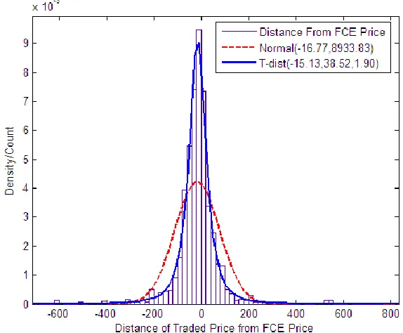
Figure 2.11: Distribution of Trade Prices Around FCE Price ... 61

Figure 2.12: Distribution of Trade Prices Around the TE Price ... 62

Figure 2.13: Distribution of TE Prices Around the FCE Price ... 62

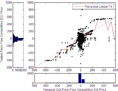
Figure 2.14: Scatter Plot of Trade Price Deviations vs. TE Price Deviations from FCE ... 63

(10)

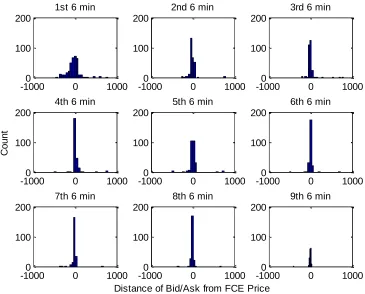
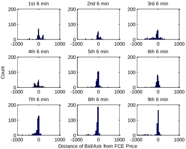
Figure 2.16: Distribution of Bids/Asks from FCE after Parameter Shift ... 73

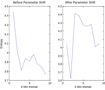
Figure 2.17: The Informational Entropy of Offer Price Distributions ... 74

Figure 3.1: Market-071208 ... 86

Figure 3.2: ACF and PACF’s of Price Changes and Squared Price Changes from Experiments 070208 Through 071208... 90

Figure 3.3: The Effect of Excess Demand for Varying Levels of dt... 94

Figure 3.4: Limit Order Book Friction as a Function of Order Book Depths ... 96

Figure 3.5: Variables Used in Classical Models of Price Adjustment ... 100

Figure 3.6: Typical Flow Competitive Supply and Demand Curves for Experiments 071205 & 071208 ... 113

Figure 3.7: Waiting Times and Acceptance Probabilities for Incentives by Rent ... 123

Figure 3.8: Waiting Times until Incentives Transacted in Public Market ... 124

Figure 4.1: Supply and Demand Curves ... 131

Figure 4.2: Speculation Between low and High Equilibria ... 132

Figure 4.3: Rate of Speculation ... 135

Figure 4.4: All Experiments and Inventories ... 143

Figure 4.5: All Experiments and Inventories per Trader ... 144

(11)

List of Tables

Table 1.1: Parameter Values under Competing Theories ... 6

Table 1.2: Quoted and Effective Spreads... 12

Table 1.3: Estimated Parameters for ASX Stocks ... 15

Table 1.4: Summary of Effects: Bid, Ask and Spread Equations ... 25

Table 1.5: Summary of Effects: Quantities Offered at First Five Levels of Bid Order Book (QD1-QD5), Quantities Offered at First Five Levels of Ask Order Book (Q1-Q5) ... 32

Table 2.1: Theories of Trader Behavior ... 51

Table 2.2: Summary of Experiments ... 56

Table 2.3: FCE and TE in Forecasting Price Movement... 65

Table 2.4: Efficiency ... 70

Table 3.1: Summary of Experiments ... 85

Table 3.2: Limit Order Book Friction as a Function of Order Book Depths ... 96

Table 3.3: Estimation of Equations 3.7a-f ... 103

Table 3.4: BIC for Classical Models ... 106

Table 3.5: Maximum Likelihood Estimation of Equations 3.8a-b ... 109

Table 3.6: The Nested Model ... 111

Table 3.7: Predicting Price Changes Based upon Inframarginal and Extramarginal Components of Excess Demand ... 115

Table 3.8: Cox Proportional Hazard Model Results ... 120

Table 4.1: Competing Theories of Information Diffusion ... 134

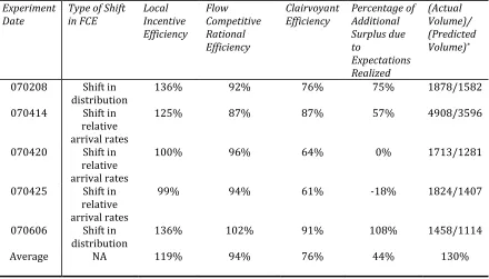
Table 4.2: Experimental Results ... 139

Table 4.3: Predicting Prices Based on Competing Equilibria ... 141

Table 4.4: Inventory Accumulation Rate of Uninformed Traders ... 146

Table 4.5: Inventory Accumulation Rate of Uniformed Traders ... 147

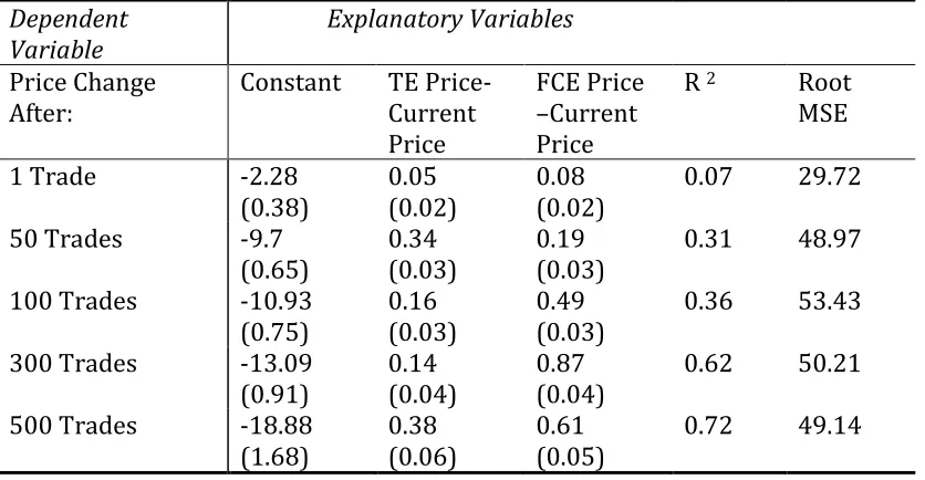
Table 4.6: Effect of Signed Run Size on Traded Prices ... 149

(12)

Introduction

In continuous double auction markets, three fundamental forces are responsible for the movement of prices, immediate incentives, expectations, and information. This thesis explores each of those three forces. Many theories in the market microstructure literature have tended to focus on common value and/or informational aspects of the double auction market rather than its ability to find supply and demand equilibria. This is due to the continuous double auctions’ application in financial markets, as well as the belief that supply and demand parameters can create an “induced common value,” making the specification of supply and demand itself relatively unimportant.

Despite this theoretical focus in the literature, this thesis shows that commonly applied models of information diffusion fail to capture key aspects of price movement in the Australian Stock Market and in experimental continuous double auction markets. Moreover, the amount of variance in intraday price movements explained by

asymmetric information is remarkably small.

(13)

Classical economics theory has prices determined by the preferences of agents

assuming that the information revealed in market responses accurately reflects both the agent’s preferences and information. This theory says very little about the details of the actual price formation process. The second theory is derived from finance in which prices are determined by the order flow coming to the market but the connection between this order flow and the underlying preferences is left abstract. Thus, this theory is not so much about equilibrium price discovery as it is the dynamics of the price making process. The role of the background incentives plays no role in this theory.

The new experimental environment lends itself to the study and integration of these two different bodies of theory. We show that in such markets, two competing generalizations of the Walrasian equilibria exist, each with an independent pull on market prices. One, which we call the flow competitive equilibrium, is similar to the classical law of supply and demand as found in economics. The other, which we call the temporal equilibrium, is similar to the price placing strategies and market

microstructure found in finance.

By modeling supply and demand as a flow of short-lived incentives, we are able to demonstrate that multiple generalizations of the Walrasian equilibrium exist in continuous random arrival markets, and show differences in levels of market efficiency between those equilibria. Prices and efficiencies reveal a strong roll of expectations in price discovery. We reject the idea that convergence is due to random or

(14)

The random arrival environment differs from traditional experimental

environments in which incentives to trade are provided at the beginning of a number of (possibly overlapping) periods. The final chapter of the thesis also explores the role of asymmetric information in this environment.

The thesis asks fundamental questions such as, Do continuously evolving markets converge to supply and demand equilibria? How does this process happen? Which classical models best explain price dynamics? And how does information become incorporated into prices and efficiencies?

Key findings include:

 Multiple generalizations of the Walrasian equilibria exist in random arrival markets.

 Convergence to supply-demand equilibria is possible in continually evolving markets without the need for repetition.

 Prices in continuous double auctions are highly influenced by local or temporary imbalances in supply and demand. This is in contrast to predictions made by rational expectations with risk neutral agents.

 The ability of continuous double auctions to converge, as well as their tendency for prices to be influenced by local factors, is best explained by a kind of

(15)

 On the other hand, expectations about future order flow do form and help to smooth prices and raise efficiency to levels that would be impossible with zero-intelligence agents.

 Measures of informational efficiency based on price convergence and measures based on efficiency levels can differ widely when applied to flow environments.

 The impact of asymmetric Information, when measured using the Ho/Stoll model, in both the Australian stock market and experimental random arrival markets with competing insiders is either small or non-existent. The proportion of variance in price changes explained by signed order flow is typically less than 10%.

 Experimental evidence from random arrival markets suggests that one possible explanation for this is that insiders hide their identities by placing both market and limit orders.

 If uninformed traders have well defined supply and demand functions, information held by insiders about the level of future prices is partially transmitted to uninformed traders through the rate of trade. This allows uninformed traders to speculate in the direction of insiders’ information, but does not actually allow them to fully learn what insiders information is.

Chapter One: Inventory and Adverse Selection Effects in a Limit Order Market

(16)

for the informational content of signed order flow, making the prior probability of a reversal in trade initiation greater than or equal to .5. This however, is not the case. Empirically, trade initiation in the Australian stock market is positively correlated, even after accounting for standard explanations of this phenomenon. Consequently, standard methods of estimating the effects of asymmetric information and inventory

management on asset prices fail to yield interpretable results. In this chapter, we estimate the impact of adverse selection and dealer inventory effects by looking at runs in trade initiation. We conclude that inventory effects are significant even in non-dealer markets, although their effect is limited to the level of the bid-ask spread. Asymmetric information has a smaller impact on the level of the bid-ask spread, but does affects the depth of the market, and the slopes of the limit order books.

 Inventory effects are significant even in non-dealer markets.

 Asymmetric information has a smaller effect on prices than inventory effects, but does affect the curvature of the limit order book.

Chapter Two: Principles of Continuous Price Determination in an Experimental

Environment with Flows of Random Arrivals and Departures studies an experimental continuous double auction environment with no asymmetric information. The period structure of classical experimental markets, which is known to play an important role in the equilibration process, is replaced by an environment in which incentives arrive randomly and continuously throughout. We show that in such markets, the focus on a single law of supply and demand is incomplete. There exist two competing

(17)

prices. The first we call the “Temporal Equilibrium,” which is based on the parameters that exist in the market at a moment in time and the second is the “Flow Competitive Equilibrium,” which reflects the underlying probabilistic structure of the parameters.

Human subjects are also able to achieve much higher levels of surplus extraction than would be possible from naïve trading strategies alone, though far less than 100% of the additional surplus due to expectations is realized. In particular, the amount of

surplus due to expectations that traders are able to extract seems to be related to the strength of public signals regarding price changes. When shifts in the FCE price are due to changes in the distribution of latent incentives, subjects tend to extract more additional surplus due to expectations than when shifts are due to changes in the relative rates of arrivals.

The distance to the FCE and TE prices are the most important variables

predicting both the location of new bids and asks as well as the probability of a bid or ask improvement. Large under pricings relative to either equilibrium concept are likely to result in a faster rate of market orders on the buy side, higher bid prices, and a greater chance of bid improvement. Similarly large over pricings relative to either equilibrium are likely to result in a faster rate of market orders on the sell side, lower ask prices, and a high chance of ask price improvement.

(18)

informational entropy, becomes more concentrated around the FCE price. Such changes in the distribution of bids and asks may be viewed as evidence of the formation of expectations.

 Trading in experimental RA markets generates high levels of efficiency relative to the maximum amount of surplus available. Realized surplus extraction is typically higher than the amount that could be obtained without speculation.

 Waiting times between trades are uncorrelated, and have a mean rate of transaction larger than the rate of transaction predicted by the FCE.

 The law of one price, in the sense of a constant price over time, does not emerge under conditions of a constant FCE price.

 Traded prices are distributed around both FCE and TE prices.

 When trade prices deviate from the FCE price, they tend to deviate in the direction of the TE price.

 Both the direction of temporal equilibrium prices and the direction of the FCE price influence price movement.

 Over time, human subjects place bids and asks closer to the FCE price. This process likely aids convergence.

Chapter Three: The Dynamics of Price Adjustment in Experimental Random

(19)

we nest all six models into a single equation, a clear winner emerges. Prices appear to move in direct proportion to the distance between the current price and the Temporal Equilibrium Price.

The distance to the temporal equilibrium appears to be the most important classical variable for several reasons. First, price dynamics are influenced only by the inframarginal portion of excess demand. Second, the speed with which individuals act on private incentives, and transact in the market is sensitive to the amount of profit available on each incentive at the current market prices. Incentives with higher rents at current offer prices were accepted faster in traders’ private markets, traded quicker in the public market, and had higher probability of being acted on in general.

Such findings support the hypothesis that market convergence is in part aided by the “probabilistic Marshallian Path,” that is, the idea that trades will form along the Marshallian path with greater probability than would occur by randomness alone.

The chapter also finds a significant role of price friction in price adjustments caused by the limit order book. The size and existence of the limit order book and the bid-ask spread also contribute to the occurrence of conditional heteroskedasticity in traded price time series.

 Price changes are relatively insensitive to excess demand between individual trades due to limit order book friction.

(20)

performs comparably well, followed by Excess Rent a distant third. (2) All of the non-fundamental models, including the classical Walrasian model individually explain less than 1% of the total variation in price changes.

 After adjusting for order book friction, auto correlation, and heteroskedasticity, there is little difference between models in terms of log likelihood.

 Significant levels of order book friction are observed for every single-variable model.

 A significant portion of heteroskedasticity is explainable by the size of the limit order books and the bid-ask spread.

 When all of the theoretically important variables are included in a single nested model, only the distance to the temporal equilibrium and potential gains from trade are statistically significant in predicting price adjustment. 2) Of the two significant variables, only the distance to the temporal equilibrium price is found to be significantly positive.

 Price dynamics are influenced only by inframarginal excess demand.

 The speed of transaction for units at the bid and ask price is influenced by the amount of rent available to the opposite side of the market at that price. The higher (lower) a bid (ask) is, the faster a transaction will occur at that price.

(21)

Chapter Four: Experimental Random Arrival Markets with Competing Insiders

studies an RA environment in which some traders have asymmetric information regarding the distribution of latent incentives and arrival rates. Theory suggests that when more than one insider has identical information, insiders will price compete, eliminating all informational rent. We find instead, that insiders do not perfectly compete and that much of the information held by insiders is incorporated in non-informed traders’ market actions. This diffusion of information is not a result of cumulative signed order flow, as predicted by theories of pure common value double auctions.

 Informational efficiency in random arrival market experiments with competing insiders is high, though typically below 100%. Approximately one third of information surplus accrued to insiders.

 Traded prices typically did not stabilize to the full information price. Hypothesis 2 is correct. Prices were slightly more likely to be found between the full

information price and the FCE price.

 The inventory buildup of uninformed traders mirrors the inventory buildup of insiders.

(22)

 The only significant determinant of inventory accumulation for uninformed subjects is the lagged total rate of speculation.

 The aggregate rate of insiders depends on location of the FCE price relative to the FIP. When the FCE is below the FIP, insider have a positive rate of inventory accumulation. When it is above the FIP, insiders have a negative, rate of

inventory accumulation.

 Insiders are also affected by competition, accelerating their rate of inventory accumulation in direct response to past rates of accumulation.

 Informed subjects submitted both market and limit orders in the same proportion as uninformed traders.

(23)

Chapter 1 Inventory and Adverse Selection Effects in a

Limit Order Market

1.1 Introduction

This chapter looks at market microstructure data for a random sample of 10 Australian stocks from the S&P/ASX 200 from Jan 2006 to Mar 2006. We find that existing models of the bid-ask spread, when applied to microstructure data, fail to identify inventory holding cost and adverse selection components of the spreads, as well as misestimate effective spreads. We modify the basic methods of (Huang & Stoll, 1997) and apply our model to runs in trade initiation in order to decompose order processing, inventory, and adverse selection effects on the level and size of the bid-ask spread as well as determine how the depth and slope of the limit order books relate to these factors.

We find evidence that dealer inventory effects on the level of the spread exist even in limit order markets and that these effects are larger than those of adverse selection. Inventory effects do not appear to persist beyond the level of the spread, while adverse selection effects tend to affect the thickness of the limit order book, decreasing the depth of the market. Because bid and ask prices are revised separately in dealer markets, asymmetries in the effects of adverse selection can be seen between bid and ask prices. Quote prices respond more strongly to unexpected order flow shocks on the same side of the market, while changes in the inventory of limit order placers effects both quotes symmetrically.

(24)

literature by highlighting the importance of runs in trade initiations and the asymmetries in the behavior of the bid and ask order books.

Most of the empirical microstructure literature related to limit order markets has focused on predictable patterns in order flow and the interactions between volume, market depth, liquidity, and volatility (Bias, Hillion, & Spatt, 1995), (Danielson & Payne, 2001), (Ahn, Bae, & Chan, Limit Orders, Depth and Volatility: Evidence from the Stock Exchange of Hong Kong, 2001), (Bollerslev & Melvin, 1994). While these studies shed valuable light on the formation of limit order books and their impact on price

movements and volatility, the literature has largely ignored issues such as the role of inventory holding costs, or to what extent components of the bid-ask spread influence the shape of the limit order book.

In part, inventory effects have been ignored in limit market order books because economists have questioned the relevancy of models of dealer inventory in non-dealer markets. Instead, theories of the spread specific to limit order markets have focused on the role of heterogeneity in traders’ demand for immediacy, and the relative arrival rates of limit and market orders (Foucault, 1999), (Foucault, Kadan, & Kandel, 2003). Empirical works have tended to attribute order flow effects on price movement as stemming entirely from asymmetric information (Bias, Hillion, & Spatt, 1995), (Chan, 2005).

(Bias, Hillion, & Spatt, 1995) study the patterns of order flow in the Paris Bourse. They find that order flow is mainly concentrated at or near the best bid and best ask price, and that rates of limit order submission are negatively correlated with market thickness. Biais, Hillion, and Spatt also note that large trades on one side of the market are likely to cause changes in the level of the bid-ask spread, a result that they attribute to asymmetric information.

(Danielson & Payne, 2001) on the other hand, provide motivation for the

existence of inventory effects and evidence of the importance of runs in trade initiation. They note that liquidity supply temporally clusters on one side of the market and

(25)

seeing fresh liquidity at the front of the other side of the book and lower chances of seeing subsidiary liquidity supply on that side of the book.

Section 1.2 of the chapter discusses the background theory of the bid-ask spread and the decomposition of its components. In Section 1.3, we discuss the characteristics of the Australian Stock Exchange (ASX) data and argue for the applicability of theories discussed in Section 1.2. In Section 1.4, we show how existing models of the effective and quoted spread fail to fit the data. We point out problems related to the tendency for trade initiation to remain on the same side of the market, and sketch the

relationship between accumulated order flow and the probability of a reversal in trade initiation. Section 1.5 modifies the basic trade indicator model for spread decomposition into a VAR model of trade initiation runs. The results of this modified model are

presented in Section 1.6. Section 1.7 concludes the chapter.

1.2 The Theory of the Bid-Ask Spread

1.2.1 Effective Spreads and Quoted Spreads

Two types of transaction costs exist in financial markets, quoted spreads and effective, or realized spreads. Quoted spreads are defined as the difference between the best asking price and the best bidding price. Today, quoted spreads can be observed in many different markets with reasonable amounts of accuracy. On the other hand, an effective spread is only realized when initiation of trade switches sides of the market and is defined as the amount that prices move due to the spread, at the times at which initiation changes.

(26)

A simple example of the difference between quoted and effective spreads is the following. Suppose a market maker sets bid and ask prices of $2 and $3 respectively. During the first half of a day, ten people each sell one unit at the bid price. Afterward, the market maker sets new bid and ask prices at $1 and $2 respectively. Ten more people now buy one unit each at the ask price. Although the quoted spread was constant throughout the day, the $1 quoted spread was never realized since everyone bought and sold at the same price; hence, the average effective spread was zero.

1.2.2 The Roll Model of the Effective Spread

(Roll, 1984) provides a model for estimating the effective spread using the auto covariance of price changes, which is commonly applied in markets where the sequence of trade initiations is unknown. Roll assumes that in an efficient market, the probability of a trade occurring at the bid price is .5 and independent of past transactions. He argues that in such a market with only an order processing component of the spread, the movement of transaction prices between the bid and the ask creates negative first order auto covariance of transaction price changes. Using this relationship, Roll derives a simple estimator of the effective bid-ask spread:

) 1 . 1 ( ) , cov( *

2 1

^



  

 t t

Roll P P

S

(Choi, Salandro, & Shastri, 1988) generalized the Roll model by allowing for the possibility of serial covariance in the sequence of trade initiations—that is, the

probability of the next trade being initiated at the bid (ask) price given that the last trade occurred at the bid (ask) price may differ from .5. Choi, Salandro, and Shastri reasoned that the conditional probability of a continuation might be larger than .5 because large market orders often initiate trades with more than one participant on the other side of the market. This causes single trades to be recorded as multiple sequential trades in ticker tape output. Choi, Salandro, and Shastri, derive a modified Roll

estimator:

) 2 . 1 ( ) ,

cov( 1

^

 

  

 t t

CSS

P P S

(27)

1.2.3 Glosten/Milgrom and Ho/Stoll

(Glosten & Milgrom, 1985) suggested a model in which some traders have inside information regarding the common value of an asset. In their model, the bid-ask spread reflects the amount that market makers must be compensated for constantly trading against informed traders. In Glosten and Milgrom, market makers adjust price levels to reflect information contained in order flow. If the last transaction occurred at the ask price, the market maker revises his or her expectation of the asset’s value upward, moving bid and ask quotes up accordingly.

(Glosten, 1987), and (Glosten & Harris, 1988) consider the possibility that the bid-ask spread reflects a combination of an order processing cost, as discussed by Roll, and an adverse selection component, as discussed by Golsten and Milgrom. Glosten and Glosten and Harris claim that the Roll estimator reflects a “gross profit” condition—the profit made by market markers above and beyond the losses they receive from trading with informed traders. Because of the way information contained in order flow causes market makers to revise prices, Glosten and Glosten and Harris show that even though the adverse selection component inflates spreads, it does not contribute negative auto covariance. Therefore, they claim that the difference between observed quoted spreads and the effective spread estimated using Roll is due to adverse selection.

(Ho & Stoll, 1981) provide an alternative explanation for why quoted spreads might be larger than effective spreads. They present a model in which dealers have an ideal level of inventory holdings, which they try to maintain. After a dealer sale

(purchase), the dealer will adjust prices upward (downward) to induce a dealer purchase (sale). Unlike adjustments due to information in Glosten and Milgrom, these

adjustments do contribute negative serial covariance.

If quoted spreads reflect a combination of all three transactions costs: order processing, adverse selection and inventory holding costs, then the difference between observed and effective spreads reflects both adverse selection and inventory

(28)

1.2.4 The Stoll Decomposition of the Quoted Spread

(Stoll, 1989) shows that five parameters summarize the differences between the order processing, adverse selection, and inventory holding cost models of the bid-ask spread:

1. δr: the amount traded prices move when there is a reversal in trade initiation 2. δc: the amount traded prices move when trade continues on the same side of

the market.

3. π: the probability of a change in trade initiation

4. Covt: the first order covariance of transaction price changes

5. Covq: the first order covariance of quote price changes, which Stoll claimed could be estimated from either the bid or ask time series1

The values for each of these parameters under the competing theories are listed in Table 1.1.

Table 1.1: Parameter Values under Competing Theories

Determination of Quoted Spread δc δr π Covt Covq

Only Order Processing

(Roll1984)

0 S 0.5 -0.25S2 0.0

Only Adverse Selection

(Copeland, Galai 1983, Glosten, Milgrom1985)

0.5S 0.5S 0.5 0.0 0.0

Only Inventory Holding Cost

(Ho, Stoll 1981)

0.5S 0.5S 1>π>0.5 -0.25S2<

S2(1-2π)- π2(1-S)

<0.0

-0.25S2<

S2(1-2π)

<0.0

Stoll’s major contribution to the bid-ask spread literature was to notice that if the quoted spread was composed of a linear combination of an order processing cost, an adverse selection component and an inventory holding cost:

) 3 . 1 ( )

1 (

sing AdverseSelection InventoryHolding s

orderproce S S

S

S    

then Equation (1.3) and Table 1.1 define a system of equations that can be solved for the relative proportions of each component of the quoted spread. Stoll estimates the

1_{Stoll (1989) used the covariance of bid prices. As Table 3 shows, the assumption that the covariances of}

(29)

parameters from daily NASDAQ data and concludes that about 47% of the bid-ask spread is comprised of order processing costs, 43% adverse selection cost and 10% inventory holding costs.

(Huang & Stoll, 1997) generalized the methodology of (Stoll, 1989) using trade indicator models to estimate the components of the bid-ask spread for NYSE data. In their model, the “true” public information price of a stock evolves according to:



[ | ]



, (1.4)

2 innovation n informatio public inventory in change Unexpected 2 2 1 1 1 1 t t t t t t t I I E I S V S V V               

Where It is an indicator function equal to 1, if a trade is designated as being buyer

initiated, and -1 if seller initiated. This specification follows from the assumption that all

trades are of unitary size. The expected change in inventory is simply:

(1.5) reversal a of y probabilit the is where , ) 2 1 ( ] |

[It1 It2    It2 

E

The midpoint of the spread Mt, is assumed to be linearly related to the order flow imbalance experienced by market makers, which is simply the sum of the indicator functions. This comes from the model of (Ho & Stoll, 1981). In that model, the dealer’s response to a change in inventory is given as the solution to a stochastic differential equation. Ho and Stoll do not solve this equation in the general case, or even show that there exists a solution to the general case. Instead, the conclusion that market makers will adjust prices linearly with changes in inventory is the result of several simplifying assumptions. Later, we will test this linearity assumption in evaluating the model.

(1.6) 1 1



    t i i t

t V I

M 

Combining Equations (1.4) and (1.6), Huang and Stoll derive the basic trade indicator

model in which changes in the midpoint of the bid-ask spread are modeled as a function

of lagged order flow, and expected order flow.

(1.7) ) 2 1 ( 2 2 )

( _t ₁ _t ₂ _t

t I

S I

S

M      

(30)

In this model, α reflects the percentage of the half spread attributed to adverse selection, and β reflects the percentage of the half spread due to inventory holding costs. (1-α-β) is interpreted as the order processing, or gross profit component of the half spread. In order to identify all of the parameters of this model, Huang and Stoll estimate the probability of a reversal separately and provide alternative specifications of the model depending on whether the quoted spread must also be estimated from the data.

Huang and Stoll note the potential for serious problems with their model. As in (Stoll, 1989), the probability of a reversal is a crucial parameter in the trade indicator model. Huang and Stoll observe the probability of a reversal to be significantly lower than .5 in NYSE data. As a result, when the model is first estimated, Huang and Stoll find the proportion of the half spread due to adverse selection to be negative—an

impossible result.

Like (Choi, Salandro, & Shastri, 1988), Huang and Stoll assume that the problem stems from large market orders being incorrectly recorded as multiple consecutive trades. As a result, Huang and Stoll overcorrect for the problem of large trades by repeating their analysis combining all consecutive trades that occurred on the same side of the market less than 5 seconds apart. After doing this, they estimate that adverse selection accounts for about 9.6% of the spreads of NYSE stocks while the inventory component accounts for about 28.7%.

1.3 The ASX and Limit Order Markets

1.3.1 Quality and Characteristics of ASX Data

(31)

our purposes, limit orders that transact immediately are effectively market orders, and will be referred to as such. The tendency for transacting limit order to hit the best bid (ask) rather than under (over) shoot, as well as the tendency for new limit orders to appear at the current best bid or ask price suggests that traders monitor orders closely.

The data used in this study come from a proprietary dataset compiled by Capital Markets Surveillance Services Pty Limited (CMSS), which consists of every bid, ask, amend, cancellation and trade on the Australian Stock Exchange (ASX). Unlike data from US dealer markets, our data is remarkably clean. Every bid, ask, cancellation and amend is recorded and labeled according to a unique bid or ask ID number. Each trade is accompanied by a bid and ask ID and a set of flags indicating whether the transaction was initiated by the buyer (transaction occurring at the ask price) or the seller

(transaction occurring at the bid price) of the transaction and whether the trade occurred on market, off market, during the opening or closing auction, etc.

As a result, the potential problem noted by (Choi, Salandro, & Shastri, 1988), that large trades being broken up into multiple consecutive trades can result in biased

estimates of the probability of a reversal, is non-existent in the data considered in this study. All consecutive trades that are initiated at the bid (ask) price and are associated with the same bid (ask) ID number are considered a part of the same trade.

1.3.2 Applicability of Inventory and Adverse Selection Models

A common objection to the methodology of this chapter is likely to be that the models of Roll, Glosten and Milgrom and Ho and Stoll, which we are applying to ASX data, are not specifically theories regarding limit order markets. While this is true, these theories are not specifically models of dealer or specialist markets either. Instead, all of the theories discussed above are models of stylized fictitious worlds in which a market makers (in this case, any trader who posts a limit price not for immediate execution) post fixed prices and individuals trade in unitary quantities with zero transaction risk.

(32)

the market maker is a single monopolist or a group of competing market makers.

Moreover, in Stoll’s seminal paper on decomposing the effects of inventory and adverse selection, he uses data from the NASDAQ, which is a multiple dealer market. Even specialists are not monopolists. On average, NYSE specialists are involved in only 26% of all trades by volume (Hasbrouck & Sofianos, 1993).

The main substantive difference between limit order markets and dealer markets is not the monopoly power of the specialist but is the degree of market

transparency and transaction risk. While some microstructure theories, such as (O'Hara & Oldfield, 1986), explicitly model the lack of transparency in dealer markets, the theories of Roll, Glosten and Milgrom, and Ho and Stoll are general enough that they do not account for order book transparency at all.

Whether market transparency is an important factor in determining bid-ask spreads is addressed in (Bortoli, Frino, Jarnecic, & Johnstone, 2006). Bortoli et al

examine a natural experiment in which the Australian Futures Exchange made an institutional change toward greater order book transparency. The exchange increased the number of visible levels of quantity on the order book from the quantity available at the best bid and ask price to the quantities available up to three ticks away from the best offers in both directions. Measuring the average sizes of the bid-ask spread before and after the change, Bortoli et al. concluded that transaction risk does not affect quoted spreads, although it did reduce the depth of the market available at the best bid and ask.

1.4 Empirical Inconsistencies of the Roll and Stoll/Huang Stoll

Models

1.4.1 Quoted and Effective Spreads in ASX Data

(33)

spread persisted, or use inter-trade quotes as well. Weighting by time does not appear to affect our estimate of the average quoted spread in any significant way. The use of inter-trade quotes in the calculation as well tends to result in higher spread estimates since there is typically a time delay between when an order is lifted off the book and the time that quantity is replaced by another limit order. Using inter-trade quotes will produce positive bias in estimates of average quoted spreads related to the frequency with which limit order placers monitor a particular stock.

(1.8) ] [#

1

_

_

 B

t A t

quoted P P

trades of S



 







        



_ _ price bid the ask to the from reverses trade if 0 price ask the to bid the from reverses trade if 1 (1.9) , 1 ] [# 1 1 1 t t B t A t t B t A t effective Z where Z P P Z P P reversals of S

For each stock, Table 1.2 lists the average quoted spread, the effective spread and two estimates of the effective spread obtained using the methods of (Roll, 1984) and (Choi, Salandro, & Shastri, 1988) . Table 1.2 also shows the price level of each stock at the beginning of the study and its average daily volume.

The actual and effective bid-ask spreads for all stocks tend to remain close to the minimum tick size of $0.01. Spreads exhibit some relationship to price levels, and

possibly vary with trading volume as well; however, there is simply not enough data to make definite conclusions regarding either statement. The spread calculations in Table 1.2 also point out why expressing spreads in terms of returns may be problematic. If quoted and effective spreads remain close to the minimum tick size for all stocks, expressing them as fractions of a stock’s share price artificially inflates the difference between the spreads of high and low priced stocks.

(34)

Table 1.2: Quoted and Effective Spreads

Stock Average Quoted Spread Effective Spread Effective/ (Average Quoted Spread) Roll Estimate of Effective Spread Choi, Salandro, Shastri Price (on 01/03/06) Daily Vol

MBL $0.0284 $0.0179 0.630 $0.0250 $0.0191 $68.00 145,679

NWS $0.0156 $0.0086 0.551 $0.0098 $0.0073 $22.69 475,942

ANZ $0.0152 $0.0080 0.526 $0.0101 $0.0077 $23.90 1,083,877

BBG $0.0200 $0.0112 0.560 $0.0124 $0.0100 $14.50 321,130

AWC $0.0117 $0.0065 0.556 $0.0072 $0.0057 $7.44 2,488,957

IVC $0.0158 $0.0103 0.652 $0.0087 $0.0082 $4.11 53,389

QAN $0.0106 $0.0075 0.708 $0.0069 $0.0058 $4.04 3,564,751

WPL $0.0239 $0.0156 0.653 $0.0214 $0.0161 $39.25 854,692

ZFX $0.0139 $0.0072 0.518 $0.0089 $0.0069 $7.00 3,126,523

GWT $0.0142 $0.0082 0.577 $0.0078 $0.0066 $3.00 123,676

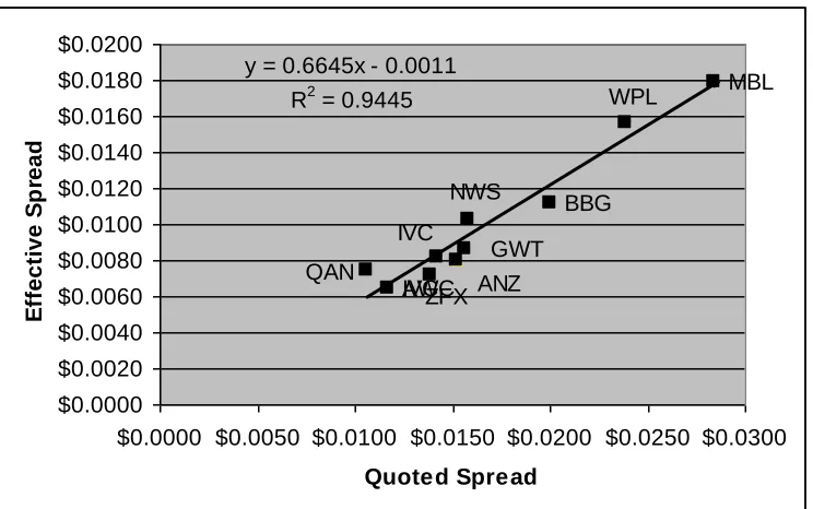
[image:34.612.113.485.430.663.2]

When Roll’s estimator is computed using per-trade transactions data, Roll tends to underestimate quoted spreads while overestimating effective spreads. On average, Roll overestimates effective spreads by about 60% using transaction data. This improves when using the modification suggested by Choi, Salandro, and Shastri. Their estimator, however, still overestimates effective spreads by about 20%.

Figure 1.1: Quoted and Effective Spreads

MBL BBG AWC IVC NWS ANZ QAN WPL ZFX GWT y = 0.6645x - 0.0011

R2 = 0.9445

$0.0000 $0.0020 $0.0040 $0.0060 $0.0080 $0.0100 $0.0120 $0.0140 $0.0160 $0.0180 $0.0200

$0.0000 $0.0050 $0.0100 $0.0150 $0.0200 $0.0250 $0.0300

(35)

Figure 1.2: Effective Spreads and Roll Estimator Using Transactions Data

Figure 1.3: Effective Spreads and CSS Estimator Using Transactions Data

y = 1.5886x - 0.0042 R2 = 0.935

$0.0000 $0.0050 $0.0100 $0.0150 $0.0200 $0.0250 $0.0300

$0.0000 $0.0050 $0.0100 $0.0150 $0.0200

Effective Spread

R

ol

l

E

s

ti

m

a

te

(

Tra

ns

a

c

ti

on

)

y = 1.182x - 0.0026

R2 = 0.9719

$0.0000 $0.0050 $0.0100 $0.0150 $0.0200 $0.0250

$0.0000 $0.0050 $0.0100 $0.0150 $0.0200

Effective Spread

C

ho

i,

S

a

la

nd

ro,

S

ha

s

tr

i

E

s

ti

m

a

(36)

1.4.2 Explaining Differences Between Quoted and Effective Spreads

In order to explain the difference between quoted and effective spreads, we first try to adopt Stoll’s (Stoll, 1989) methodology to estimate the size of the relative

components of the quoted spread. For each stock, we use bid, ask, and transaction prices along with the observed sequence of trade initiations to estimate the parameters given in Table 1.1. We allow δc, δr and π to differ depending on whether the last trade was initiated at the bid (δcb, δrb, πb) or ask price (δca, δra, πa), and estimate the

covariance of quote prices for bid and ask price time series separately.

(37)

Table 1.3: Estimated Parameters for ASX Stocks

Stock δcb δca δrb δra πb πa Covt Covb Cova

MBL -$0.0078 $0.0064 $0.0152 -$0.0166 0.4681 0.3891 -1.56E-04 -1.22E-04 1.39E-04

NWS -$0.0024 $0.0033 $0.008 -$0.0072 0.4046 0.5086 -2.42E-05 -7.39E-06 -2.91E-06

ANZ -$0.0028 $0.0026 $0.0071 -$0.0075 0.4679 0.4001 -2.57E-05 -5.53E-06 -1.52E-06

BBG -$0.0041 $0.0045 $0.0084 -$0.0086 0.3788 0.3873 -3.84E-05 -1.99E-05 6.75E-07

AWC -$0.0016 $0.0015 $0.006 -$0.0059 0.4061 0.3934 -1.30E-05 -3.14E-06 2.75E-04

IVC -$0.0014 $0.0019 $0.0093 -$0.0092 0.2625 0.3091 -1.90E-05 -1.25E-05 -8.61E-06

QAN -$5.45E-04 $5.26E-04 $0.0076 -$0.0073 0.3129 0.4054 -1.20E-05 -4.97E-04 -1.41E-05

WPL -$0.0062 $0.0057 $0.0131 -$0.0139 0.4725 0.4103 -1.14E-04 -0.0296 0.0013

ZFX -$0.0021 $0.0019 $0.0067 -$0.0066 0.4387 0.3885 -1.97E-05 -2.28E-06 -7.24E-07

GWT -$0.001 $0.0019 $0.0084 -$0.008 0.2648 0.4193 -1.50E-05 -2.71E-06 -1.66E-06

Ask covariances tend to be higher than bid covariances because of the way stock prices adjust. Contrary to theory, quote prices do not adjust simultaneously. One price often undergoes multiple sequential revisions in one direction before the other price adjusts once. Because stock prices tend to move upwards, ask price changes are more likely to accumulate positive auto covariance than bid prices.

Figure 1.4 illustrates a sequence of trades for MBL during a period of price adjustment. Stock prices adjust upward when a large number of trades initiated by buyers erode limit orders on the other side of the market. This erosion of ask orders pushes the ask quote upward, but more importantly, it causes ask prices to rise at a faster rate than bid prices, increasing the quoted spread.

(38)

Figure 1.4: Upward Price Adjustment in MBL

1.4.3 The Tendency for Reversals

A natural question to ask given the low probability of a reversal is whether the probability of a reversal is increasing with the accumulated size of a continuation. It may be that markets have an “order flow threshold.” That is, small trades, even groups of small trades on the same side of the market are unlikely to induce any revision of prices. Only if a large enough order arrives or if a run of small trades accumulates enough one-sided order flow, will markets undergo a price adjustment.

(39)

Figure 1.5 below shows the typical shape of the relationship between the current size of a run and the instantaneous probability of a reversal. The estimated hazard rate functions of the stocks in this sample reveal that there is indeed a relationship between how long a continuation has already lasted and its instantaneous probability of ending. In general, the longer a run has continued, the more likely it is to end, although this relationship appears weak for a broad range of run sizes at the beginning of the distribution of run sizes.

Essentially, many small trades can accumulate on one side of the market before affecting the probability of a reversal in a meaningful way. As orders build up on one side, however, the probability of a reversal increases at a faster rate as orders in a run arrive.

(40)

1.5 Methodology

1.5.1 Predicting Changes in the Level and Slope of the Order Book

Given the problems associated with the tendency for continuations in trade initiations, we propose a modification of the Huang and Stoll trade indicator model in which the probability of a reversal is set to one. Specifically, consider the sequence of trade initiations and quantities:

Trade Indicator

1 1 1 -1 -1 1 -1 -1

Quantity

of Shares 100 300 200 500 100 300 200 100

Instead of looking at individual trades, we look at the alternating sequence of runs, measuring the size of the spread, the change in the level of the spread, and the depth of the market at and around the best ask and best bid on the limit order book between every run. The sequence of individual trades represented above then becomes the sequence of runs below:

Trade

Indicator 1 -1 1 -1

Quantity

of Shares 600 600 500 200

We then make similar assumptions regarding the effect of order flow on the true value of the stock and the relation between order imbalance and the “true” value of the stock. We assume that the change in the true price of a stock is a linear function of the size of the previous run, measured in shares, and the unexpected shock in order flow, also measured in shares. Similarly, we assume that the level of prices is a linear function of the true value and the size of the previous run. While Huang and Stoll focus on the mid point, we model changes in bid and ask prices separately in order to explore potential asymmetric effects on the spread.

(41)



₁ [ ₁| ₂]



(1.10)

1 t t t t

t

t V Q EQ Q

V  _  _  _ _ 

We estimate the system of equations below where Qˆt1 is an estimate of the size of the run at time t-1, based upon information available at time t-2, and the V’s are vectors of autoregressive terms and the predicted variance ofQˆt. The vector of error terms of the system of equations is assumed contemporaneously cross-correlated while all other cross correlations are assumed zero.

Notice that in the equations below we have dropped the term S/2 from the original model. This is because we are no longer considering a fixed, point spread. By grouping all trades in a single run together, we are considering an “order flow” spread, which reflects how the interaction of market order flow and the arrival of new limit orders have changed the level of prices over the length of a trade run.





























5 5 5

1 1 5 1 5 5 1 1 1 1 1 1 1 1 1 5 5 1 1 5 1 5 5 1 1 1 1 1 1 1 1 1 1 1 1 1 1 1 1 1 1 ˆ 5 ˆ 1 ˆ 5 ˆ 1 ˆ ˆ ) 11 . 1 ( ˆ QD t QD QD t t QD t QD QD QD t QD QD t t QD t QD QD Q t Q B t t Q t Q Q Q t Q Q t t Q t Q Q S t S S t t S t S S t B t B B t t B t B B B t A t A A t t A t A A A t V Q Q Q QD V Q Q Q QD V Q Q Q Q V Q Q Q Q V Q Q Q S V Q Q Q P V Q Q Q P                                                                                                      

1.5.2 A Graphical Interpretation

(42)

After each run, we measure the amount that the price on the same side of the market as the previous trade changed. This is denoted either Yt YtAif the previous trade was at the ask price or B

t t Y

Y  if the previous run was at the bid price in Figure 1.6 below. Between each run, just prior to the start of the new run, we also measure the size of the previous run, denoted as INV in Figure 1.6, and the amount that its size differed from its predicted size, denoted AS below. Measurements of the components of the spread are obtained by regressing Y on run size and the size of the shock to determine the relative importance of the two components of the unrealized spread.

Order Processing Component Adverse

Selection _YA

t=aA+bA1ASt+bA2INVt+et Inventory

Costs

Ask Price

Bid Price

Unrealized Spread

Unrealized Spread Unrealized Spread

YBt=aB+bB1ASt+bB2INVt+et Trades

(43)

1.5.3 Predicting Expected Order Flow

In order to accurately measure the effects of adverse selection on stock prices, we must predict the size of future order flows given the information available just prior to the time of a reversal. The size of consecutive runs can be correlated for many different reasons. According to the theory we are interested in evaluating, order flows at consecutive runs are correlated because of market making activities that adjust the level of bid and ask prices in order to induce changes in inventory.

We also know from other micro market studies of order flow and liquidity that the volume of trade obeys certain predictable time patterns. For example, order flow tends to start high following the opening auction, fall off towards the middle of the day and picks back up near the close of the market. Volume is also known to differ

depending on the day of the week or month. Volume tends to be different on Mondays and Fridays as well as the first and last days of the month. The relation between volume and time of day found in this study is similar to typical U-shaped pattern of volume found in (Ahn & Cheung, 1999) and (Bias, Hillion, & Spatt, 1995).

When forecasting future order flow, it is important to distinguish between the amount of correlation in run sizes caused by market making activities, and the amount that is merely because consecutive runs are jointly influenced by the same latent variables affecting the level of volume in general. If Ho and Stoll are correct that market makers affect future order flow in response to past inventory changes, we should expect past order flow to forecast future order flow even in the presence of variables

controlling for time. Moreover, we should expect the predictive power of past inventory to be robust to the presence of time variables.

(44)

We also explore the possibility that future inventory depends on past runs deeper than the first lag. We find past lags significant in predicting run size, although the length of lagged dependence appears to extend only to the second lag.

Presumably, market makers are aware of predictable time patterns of volume, and anticipate them in their pricing. Thus, we use both sources of correlation to predict the unexpected shocks to market makers’ inventory.

We will also forecast the expected variance of future run sizes as a linear

function of the same variables used in forecasting the mean of future run size. We place no restrictions on the parameters of the variance equation to assure that the variances are positive, but verify after estimation that each observation in the sample has positive expected variance. Generally, the number of negative variance predictions is small, less than 1% of the sample size. These observations are then set to zero.

t 2 2 1 1 2 2 2 1 1 dummies h week/mont of day ) 13 . 1 ( les day variab of time changes price lagged dummies h week/mont of day (1.12) les day variab of time changes price lagged                               t t t t t t t Q Q Q Q Q

1.6 Results

1.6.1 The Level of the Bid-Ask Spread

The analysis of our data indicate that the size and level of the bid-ask spread is determined by three components: an order processing cost, which constitutes the majority of the quoted spread, an inventory cost, and adverse selection cost. The effect of inventory and adverse selection costs, as predicted by theory, are similar, both tending to move prices in the direction of the previous trade run.

(45)

the estimated effect of the variable was positive and negative, regardless of the significance of that result.

As a simple non-parametric test of the inventory and adverse selection hypotheses, we compare the number of times an effect was estimated to be positive (negative) to the probability of obtaining the same or greater number of positives (negatives) under the null hypothesis that positive and negative results are equally likely.

Theory predicts that large volume and unexpected volume at the ask price will cause prices to go up and that large volume and unexpected volume at the bid price will cause prices to go down. Ten out of ten times the effect of quantity traded at the bid price was found to have a negative effect on the bid price, and ten out of ten times the effect of quantity traded at the ask price was found to have a positive effect on the ask price. The probability of this happening by chance alone is only about 1%. We also find that quantity at the ask (bid) price had a positive (negative) effect on bid (ask) prices nine (nine) out of ten times as well, an event with about 2% probability.

Less significant results are obtained for the effects of adverse selection. Adverse selection also appears to have asymmetric effects on bid and ask prices with bid prices responding more strongly to run size shocks at both the bid and ask prices. This

asymmetry may be related to the tendency for the bid order book to exhibit a higher degree of curvature than the ask order book as the slope and curvature of the book is essentially a measure of prices’ sensitivity to volume. Unexpected shocks at the ask price had a positive effect on bid and ask prices in 7 stocks each, while unexpected shocks at the bid price had a negative effect on bid and ask prices in 8 and 10 stocks respectively.

(46)

exception to this was the effect of shocks at the ask price on the level of the bid price, for which one stock had a significantly negative estimate.

Overall, a trade run at the ask price one standard deviation larger than the mean can expect to increase bid and ask prices by slightly more than half a cent. On the other hand, a run at the bid price one standard deviation larger than the mean can expect to lower bid and ask prices by slightly less than half a cent. Because of a large amount of skewness in the distribution of run sizes, most run sizes lie somewhere between +/-1 standard deviation from the mean, but runs +5, +6, even +13 standard deviations or more away from the mean are not uncommon, certainly much more probable than they would be under a normal distribution.

The effect of observing an unexpected shock in run size one standard deviation large than the mean at the ask price tends to raise the ask price by about .3 cents, while having little impact on the immediate movement of the bid price. Similarly, a one standard deviation shock at the bid price will decrease the bid price by about .3 cents as well, and will have an effect about half that size on the ask price.

The asymmetry between how bid and ask prices respond to information contained in order flow is particularly theoretically important. Typically, theory has assumed that the bid-ask spread is either constant, or that when bid and ask prices are revised, that they are revised simultaneously. In a dealer market, where bid and ask prices are periodically announced by a specialist such as on the NYSE, this is not a bad assumption. However, in a limit order market, prices changes occur one at a time when orders at the front of the book are lifted, cancelled or improved.

In theory, inventory effects are caused by dealers’ desire to rebalance inventory— induce dealer sales after dealer purchases, and visa versa—hence, in a market where prices are revised separately, the inventory effect is an effect that betters prices on the side of the market opposite the previous trade run2. Conversely,

2

(47)

information effects are caused by dealers adjusting prices in ways that reduce order flow from informed traders, hence when prices adjust separately, adverse selection is primarily an effect that worsens prices on the same side of the market as the previous run. In light of how the two effects of information and inventory are likely to affect bid and ask prices differently, it is not surprising that we find inventory effects have a larger impact on prices on the opposite side of the market than do adverse selection effects.

Table 1.4: Summary of Effects: Bid, Ask and Spread Equations

Figure 1.7: 95% Confidence Intervals for Effect of Trade Size (at Ask Price) on Bid Price

because when the spread is small same-side price movement is a prerequisite for adjusting opposite-side prices in ways that correct inventory imbalance.

Last Run at Ask Price

Quantity Traded at Ask Price in Previous Run

Quantity Traded at Bid Price in Previous Run

(Quantity Traded at Ask Price in Previous Run)^2

(Quantity Traded at Bid Price in Previous Run)^2 Unexpect ed Shock at Ask Price Unexpect ed Shock at Bid Price Variance of Run Size Constant

dbestbid x P(X>=x|p=.5)

average 0.0050 0.0077 -0.0041 -0.0004 0.0003 -0.0002 -0.0031 0.0000 -0.0015 1 0.999 std dev 0.0027 0.0088 0.0031 0.0005 0.0004 0.0064 0.0026 0.0004 0.0024 2 0.990 min 0.0016 -0.0001 -0.0120 -0.0016 -0.0003 -0.0145 -0.0084 -0.0004 -0.0047 3 0.947 max 0.0102 0.0258 -0.0004 0.0000 0.0009 0.0069 -0.0003 0.0008 0.0038 4 0.831

# Positive 10 9 0 2 8 7 0 4 2 5 0.627

#Negative 0 1 10 8 2 3 10 6 8 6 0.382

dbestask 7 0.178

average 0.0040 0.0051 -0.0045 -0.0006 0.0002 0.0026 -0.0017 0.0001 -0.0014 8 0.062 std dev 0.0026 0.0053 0.0049 0.0007 0.0006 0.0039 0.0034 0.0006 0.0020 9 0.019 min 0.0011 0.0005 -0.0156 -0.0024 -0.0013 -0.0026 -0.0075 -0.0005 -0.0055 10 0.010 max 0.0094 0.0156 0.0000 0.0002 0.0009 0.0110 0.0049 0.0016 0.0025

# Positive 10 10 1 2 8 7 2 4 1

#Negative 0 0 9 8 2 3 8 6 9

spread

average -0.0012 -0.0017 0.0002 -0.0001 -0.0002 0.0019 0.0008 0.0001 0.0263 std dev 0.0011 0.0025 0.0012 0.0002 0.0002 0.0025 0.0018 0.0002 0.0760 min -0.0040 -0.0077 -0.0017 -0.0006 -0.0008 -0.0004 -0.0012 -0.0001 0.0006 max 0.0002 0.0005 0.0021 0.0001 0.0001 0.0077 0.0044 0.0007 0.2426

# Positive 1 3 7 3 1 8 6 8 10

#Negative 9 7 3 7 9 2 4 2 0

Effect of Trade Size (at Ask Price) on Bid Price

-$0.0100 $0.0000 $0.0100 $0.0200 $0.0300 $0.0400