Tutorial in biostatistics - Sample sizes for clinical trials with Normal data

This is a repository copy of Tutorial in biostatistics - Sample sizes for clinical trials with Normal data.

White Rose Research Online URL for this paper: http://eprints.whiterose.ac.uk/145474/

Version: Accepted Version

Article:

Julious, S.A. (2004) Tutorial in biostatistics - Sample sizes for clinical trials with Normal data. Statistics in Medicine, 23 (12). pp. 1921-1986. ISSN 0277-6715

https://doi.org/10.1002/sim.1783

This is the peer reviewed version of the following article: Julious, S.A. (2004) Tutorial in biostatistics - Sample sizes for clinical trials with Normal data. Statistics in Medicine, 23 (12). pp. 1921-1986, which has been published in final form at

https://doi.org/10.1002/sim.1783. This article may be used for non-commercial purposes in accordance with Wiley Terms and Conditions for Use of Self-Archived Versions.

Reuse

Items deposited in White Rose Research Online are protected by copyright, with all rights reserved unless indicated otherwise. They may be downloaded and/or printed for private study, or other acts as permitted by national copyright laws. The publisher or other rights holders may allow further reproduction and re-use of the full text version. This is indicated by the licence information on the White Rose Research Online record for the item.

Takedown

If you consider content in White Rose Research Online to be in breach of UK law, please notify us by

Tutorial in Biostatistics: Sample sizes

for clinical trials with Normal data.

SUMMARY

This article gives an overview of sample size calculations for parallel group and cross-over

studies with Normal data. Sample size derivation is given for trials where the objective is to

demonstrate: superiority, equivalence, non-inferiority, bio-equivalence and estimation to a

given precision, for different Type I and Type II errors. It is demonstrated how the different

trial objectives influence the null and alternative hypotheses of the trials and how these

hypotheses influence the calculations. Sample size tables for the different types of trials and

worked examples are given.

Key Words

Sample size, Power, Type I error, Type II error, Superiority trials, Equivalence trials,

Non-inferiority trials, Bio-equivalence, Precision, Baselines, Cross-over trials, Parallel group

CONTENTS

1. Introduction

1.1. Estimation of the variance for calculations

2. Superiority trials

2.1. Parallel group trials

2.1.1. Worked Example

2.1.1.1. Using the sample size tables

2.1.1.2. Repeated using sample size software

2.2. Cross-over trials

2.2.1. Paired t-tests and period adjusted t-tests

2.2.2. Sample size calculations

2.2.3. Worked Example

2.2.3.1. Using the sample size tables

2.2.3.2. Repeated using sample size software

3. Equivalence trials

3.1. General case

3.2. Special case of no treatment difference

3.3. Type I and setting the equivalence limit

3.3.1 Choice of Type I error

3.3.2. Choice of Equivalence Limit

3.4. Parallel group trials

3.4.1. General case

3.4.2. Special case of no treatment difference

3.4.3. Worked example

3.4.3.2. Repeated using sample size software

3.5. Cross-over trials

3.5.1. General case.

3.5.2. Special case of no treatment difference.

3.5.1. Worked example

3.5.1.1. Using the sample size tables

3.5.1.2. Repeated using sample size software

4. Non-inferiority trials

4.1. Parallel group trials

4.1.1. Worked example

4.1.1.1. Using the sample size tables

4.1.1.2. Repeated using sample size software

4.2. Cross-over trials

4.2.1. Worked example

4.2.1.1. Using the sample size tables

4.2.1.2. Repeated using sample size software

5. As good as or better trials

5.1. A test of non-inferiority and a one sided test of superiority

5.2. A test of non-inferiority and a two sided test of superiority

5.3. Worked example and other considerations

6. Bio-equivalence trials

6.1. Justification for log transformation

6.2. Rational for using coefficients of variation

6.3.2. Special case of ratio equalling unity

6.3.3. Replicate Designs

6.3.4. Use of quick formulae to estimate the sample size of a

bioequivalence trial

6.3.5. Worked Example

6.3.5.1. Using the sample size tables

6.3.5.2. Repeated using sample size software

6.4. Parallel Group Studies

6.4.1. General case

6.4.2. Special case of ratio equalling unity

6.4.3. Worked Example

6.4.3.1. Using the sample size tables

6.4.3.2. Repeated using sample size software

6.5. Individual and Population Bio-equivalence

7. Trials to a give precision

7.1. Parallel group trials

7.1.1. Worked Example

7.1.1.1. Using the sample size tables

7.1.1.2. Repeated using sample size software

7.2. Cross-over trials

7.2.1. Worked Example

7.2.1.1. Using the sample size tables

7.2.1.2. Repeated using sample size software

8. Design considerations

8.2. Post dose measures summarised by summary statistics

8.3. Inclusion of Baseline or Covariates as well as Post Dose Measures

9. Summary

1. INTRODUCTION

Since the first 'modern' randomised clinical trial was reported in 1948 [1], clinical trials have

become a central component in the assessment of new therapies. The primary objective of

any clinical trial is to obtain an unbiased and reliable assessment of a given regimen response

independent of any known or unknown prognostic factors. First, by ensuring that the

patients studied in the various regimen arms are objectively similar with reference to all

predetermined relevant factors other than the regimens themselves. Second, by making sure

that the assessment of the regimen response is independent of a given subject's regimen and

finally through inclusion of an appropriate control to quantify a given regimen response [2].

Randomisation is important as it ensures that patients are objectively similar in the regimen

groups being investigated for any demographic or prognostic factors that either known or

unknown [3]. Randomisation achieves this by ensuring that each subject has a known chance

of being given a given treatment in an allocation that can not be predicted [4].

Blinding is important as it removes any systematic bias there may be in treatment assessment

and allocation during the conduct of the trial. It is important too once the trial has been

completed during the cleaning and derivation of the data [5]. If there is any knowledge of

treatment during the cleaning and querying of the data then this knowledge may affect how

these data are consequently queried and cleaned [3].

The choice of an appropriate control is dependent on the objective of the trial being designed.

For example a non-inferiority or equivalence trial will usually have a control which is active

if the primary outcome is efficacy. The different types of trials will be described through this

paper.

When planning a trial one essential step is the calculation of a sample size which will give

the minimum sample size required to meet the given objectives of the study. Sample size

large may be judged unethical [6]. For example, a study that is too large could have met the

objectives of the trial before the actual study end had been reached, and so some patients may

have unnecessarily entered the trial. A trial that is too small will have little chance of meeting

the study objectives, and patients may be put through the potential trauma of a trial for no

tangible benefit. The general approach to choosing sample size will be described in this

article where a statistic can be assumed to take a Normal form and an estimate of the

variance of that test statistic is available. The sections of the paper detail computation of

sample sizes appropriate for:

1. Superiority trials.

2. Equivalence trials.

3. Non-inferiority trials.

4. As good as or better trials.

5. Bio-equivalence trials.

6. Trials to a given precision.

A distinction therefore is drawn to emphasise differences in trials designed to demonstrate

'superiority' and trials designed to demonstrate 'equivalence' or 'non-inferiority'. This is

discussed with an emphasis on how differences in the null hypothesis can impact on

calculations. The ICH guidelines E3 and E9 provide general guidance on selecting the

sample size for a clinical trial [3, 7]. The ICH E9 guideline states that:

"The number of subjects in a clinical trial should always be large enough to provide a reliable

answer to the questions addressed. This number is usually determined by the primary

objective of the trial ….The method by which the sample size is calculated should be given

in the protocol together with any quantities used in the calculations (such as variances, mean

This paper will go through the methods of sample calculation for studies with the six distinct

objectives listed above. The paper will also, under the worked examples, give a brief

description of how the calculations could be undertaken in the two packages PASS 2000 [8]

and nQuery 4 [9]. Although PASS 2000 and nQuery 4 are the only packages described in

detail this does not confer a recommendation as to their use by the author.

The paper is written on the premise that just two treatments are to be compared in the clinical

trial and two study designs will be discussed: parallel group and cross-over designs.

With a parallel group design subjects are assigned at random to the two treatments to form

two treatment groups which it is hoped are the same in all respects other than the treatment

received.

With a cross-over trial all subjects receive both the treatments but it is the order that subjects

receive the treatments which is randomised. The big assumption here is that prior to starting

the second treatment all subjects return to baseline and that the order which subjects receive

treatment does not affect their response to treatment. Cross-over trials can not be used

therefore in degenerative conditions, where subjects get worse over time. Also, they are

more sensitive to bias than parallel group designs [2].

Although this paper will concentrate on data that take a Normal form this does not limit its

scope as trials where the primary endpoint is assumed to be Normal probably account for the

majority of trials. Also, the discussion in each section on the null hypothesis for each trial

and the sample size derivation is generalisable for other types of data. For superiority trials

there is work for cross-over [10] and parallel group [11] trials where the data take other

distributional forms as well as methodologies for parallel group non-inferiority [12] and

equivalence trials [13] for binary data.

Conventions for multiple comparisons are not discussed in this paper, although the

made. Koch and Ganksy give an overview of this topic [14] whilst the CPMP have issued

guidelines [15].

Each section of the paper will walk through the derivation of the appropriate sample size

formulae. Tables are given in each section which provide sample size estimates using these

formulae and worked examples are described which use these tables. Also, within each

section quick formulae are given which do not necessitate the use of tables for calculations.

1.1. Estimation of the variance for calculations

Through out this paper one of the most important components in the sample size calculation is

the variance estimate used. This variance estimate is usually estimated from retrospective

data sometimes from a number of studies. To adjudicate on the relative quality of the

variance one should consider the following aspects of the trial from which the variance is

obtained

1. Design: is the study design ostensibly similar to the one you are designing? On the basic

level is the data from a randomised controlled trial - observational or other data may greater

variability. If you are undertaking a multi-centre trial is the variance estimated too from an

similarly designed trial? Were the endpoints similar to those you plan to use – not just the

actual endpoints but was the time relative to treatment of the outcome of interest similar to

you own?

2. Population: is the study population similar to your own? The most obvious consideration

is to ask is whether the demographics were the same but if the trial conducted was a multi

centre one was it conducted in similar countries? Different countries may have different types

of care (e.g. different concomitant medication) and so may have different trial populations.

3. Analysis: was the same statistical analysis undertaken? Not just the question of whether

the same procedure was used for the analysis but were the same covariates fitted into the

model? Was the same summary statistics used? Section 8 details how covariates and

summary statistics impact on the variance.

The quality of the variance will obviously influence the strategy of an individual clinical trial -

it has not been unknown to have next to no data on hand when designing a trial such that the

range divided by four is taken as a variance estimate. Depending on the quality of the

variance estimate (or even if one has a good variance estimate) it may be advisable to have

some form of variance re-estimation during the trial. There is a developing literature on this

2. SUPERIORITY TRIALS

In a superiority trial the objective is to determine whether there is evidence of a statistical

difference in the comparison of interest between the regimens with reference to the null

hypothesis that the regimens are the same. The null (H0) and alternative (H1) hypotheses

may take the form:

Ho: The two treatments are not different with respect to the mean response (µA =µB).

H1: The two treatments are different with respect to the mean response (µ_A ≠µ_B).

In the definition of the null and alternative hypotheses µ_Aand µ_Brefer to the mean response

on regimens A and B respectively. In testing the null hypothesis there are two errors one can

make:

I. Rejecting Ho when it is actually true.

II. Not rejecting Accepting Ho when it is actually false.

These errors are usually referred to as Type I and Type II errors [25, 26, 27, 28, 29, 30]. The

aim of the sample size calculation is to find the minimum sample size for a fixed probability

of Type I error to achieve a value of the probability of a Type II error. The two errors are

commonly referred to as the regulator's (Type I) and investigator's (Type II) risks and by

convention are fixed at rates of 0.05 and 0.10 or 0.20 respectively. The Type I and Type II

risks carry different weights as they reflect the impact of the errors. With a Type I error

medical practice may switch to the investigative therapy with resultant costs whilst with a

Type II error medical practice would remain unaltered.

In general, one usually thinks not in terms of the Type II error but in terms of the power of a

trial (1-probability of a Type II error) which is the probability of rejecting the Ho when it is in

fact false. Key trials should be designed to have adequate power for statistical assessment of

noted though that with 80% power one is doubling Type II error for only a 25% saving in

sample size.

For a superiority trial there are two chances of rejecting the null hypothesis and thus making

a Type I error. The null hypothesis can be rejected if µ_A >µ_B or if µ_A <µ_B by a

statistically significant amount. As there are two chances of rejecting the null hypothesis the

statistical test is referred to as a two tailed test with each tail allocated an equal amount of the

Type I error (of 2.5%). The sum of these tails adds up to the overall Type I error rate of 5%.

Thus, the null hypothesis can be rejected if the test of µ_A >µ_B is statistically significant at

the 2.5% level or the test of µ_A >µ_B is statistically significant at the 2.5% level.

The purpose of the sample size calculation is hence to provide sufficient power to reject Ho

when in fact some alternative hypothesis is true. One might therefore test that the two means

are equal, against an alternative that they differ by an amount 'd' [31]. The amount d is

chosen as a clinically important difference or effect size and is the main factor in determining

a sample size. Reducing the effect size by half will quadruple the required sample size [32].

Formally the aim is to calculate a sample size suitable for making inferences about a certain

function of given model parameter, µ, f

( )

( )

will be µ −A µB i.e. the difference in means of two populations A and B. Now let S be a

sample estimate of f

( )

is assuming that the data from the clinical trial are sampled from a Normal population, then,

using standard notation, S~N( f

( )

( )

( )

f

S− µ

.

A basic equation can now be developed in general terms from which a sample size can be

assigned to each tail of the two tailed test, and let Z1−α/2denote the

(

)

point of a standard Normal distribution.

Thus, an upper 2-tailed, α -level critical region for a test of f

( )

( )}

For this critical region one needs to test it against an alternative that f

( )

chosen d and specified power (1- ) [33]:

( )

d− 1_−β =Z1−α/2 Var

( )

where β is the overall Type II error level and Z_1−βis the 100(1- )% point of the standard

Normal distribution. Thus, in general terms for a 2-tailed, α -level test one has:

Var (S) = ₂

2 / 1

1 Z )

(Z

2

α

β −

− +

d

(2.2)

where Var (S) will be unknown and depends on the sample size. Once Var (S) is written in

terms of sample size, the above expressions can be solved to give the sample size.

In this section, and throughout the paper for parallel group trials, the assumption will be

made that the variances in each group are equal i.e. that 2 A

σ = 2 B

σ =σ2

. This assumption is

referred to as homoskedasticity. There are alternative derivations for the case of unequal

2.1 Parallel Group Trials

Suppose one wishes to design a two group study where the sample size in the second group,

nB, can be written as some multiple of the first, nA, (say nB= nA). Then Var (S) can be

written in terms of nA and hence equation (2.2) can be solved for nA. For example, for an

r:1 Var(S) can be derived as:

( )

2 _{σ σ}

σ

r r S

Var = + = + _(2.3)

Where σ2

is the population variance estimate. Substituting into equation (2.2) gives [35]:

(

)

= , (2.4)

where nB =rnA. Note: n=nB + nA is minimised when r = 1.

When the clinical trial has been conducted and the data has been collected and cleaned for

analysis it is usually the case that for the analysis the population variance, σ2, is considered

unknown and a sample variance estimate, s , is used instead of 2 σ2. As a consequence of

this a t-statistic as a opposed to a Z-statistic is used for inference. This fact should be

represented in the sample size calculation rewriting equation (2.4) so that t- as opposed to

Z-values are used. Hence, the following equation should be used:

d r

n_A nA r

2 ) t (Z ) 1

(r 2 2

2 ) 1 ( , 2 / 1

1−β + −α + − σ +

≥ (2.5)

where nA is now defined as the least integer values that satisfies equation (2.5). As nA

appears on both the left and write side of the equation (2.5) it is best to re-write the equation

in terms of power and then use an iterative procedure to solve for nA:

        − + Φ =

− 2 1₋ /2, ( ₊1)₋2 2

) 1 (

1 n r

A A t r d rn α σ

where Φ

( )

could use equation (2.4) for the initial sample size calculation and then calculate the power

for this sample size using equation (2.7), iterating the sample size up as necessary until the

required power is reached. However, when a sample variance is being used in the analysis

the power should be estimated from a cumulative t distribution as opposed to a cumulative

Normal [35, 36, 37]. The reason for this is that by replacing σ2 with s2 equation 2.6

becomes:         − + =

− 2 1₋ /2, ( ₊1)₋2 2

) 1 (

1 n r

A A t s r d rn P _α β

where P

( )

re-written as:         − + =

− _{2 2} 1₋ /2, ( ₊1)₋2

) 1 (

1 n r

A A t s r d rn P _α σ σ β

by dividing top and bottom by σ2. Thus, one has a Normal over a square root of a

chi-squared which by definition is t-distribution. In fact as the power is estimated under the

alternative hypothesis, and that under this hypothesis d≠0, Senn has shown specifically that

instead of a t distribution the power should be estimated from a non-central t distribution

with degrees of freedom nA(r+1)-2 and non-centrality parameter rnA (r+1)σ2 [35]. Thus,

equation 2.6 should in fact be rewritten as:

        + − + − =

− 1₋ /2, ( ₊1)₋2 2 ₂

) 1 ( , 2 ) 1 ( , Probt 1 1 σ β _α r d rn r n t A A r

n_A (2.7)

where Probt

( )

(

)

4 2

Z Z ) 1

(r 2 2 _{1 /2}

2 / 1

1−β −α σ _−α

+ +

+

= Z

d r

n_A . (2.8)

For quick calculations the following formula, to calculate a sample size, with 90% power and

a two-sided 5% type I error rate, can be used:

r r d nA

) 1 ( 5 . 10

2

2 ₊

= σ , (2.9)

or for r=1:

2 2 21

d n_A = σ .

This, 21/δ2 (δ =d/σ ) is a particularly useful result to remember for quick calculations.

Equations (2.4) and (2.8) are close approximations to equation (2.7), giving estimates only

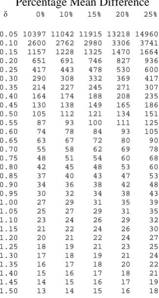
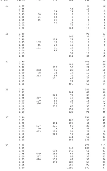
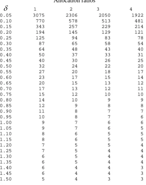
one or two lower and thus provide quite good initial estimates. Table 2.1 gives sample sizes

using equation 2.7 for various standardised differences (δ =d/σ ).

2.1.1. Worked Example

2.1.1.1. Using the sample size tables

An investigator wishes to design a hypertension trial with equal allocation between groups

where the clinical effect of interest is a reduction in blood pressure, compared to control, of

8mmHg (d). The expected standard deviation in the population in which the trial is to be

undertaken is 40mmgHg (σ ). Thus, the standardised difference equates to

20 . 0 40 / 8

/ = =

= σ

δ d . With the Type I and Type II errors fixed at 5% and 10% equation

2.8 gives a sample size of 526. Using this sample size to initiate iterations in Equation 2.7

one gets the following steps:

Iteration n Power

1 526 0.8993

Thus, the sample size required is 527 subjects in each arm of the trial and a total sample size

of 1054. Alternatively one could look up the standardised effect of 0.20 in table 2.1 which

gives the same sample size.

If the trial was designed with an unequal allocation of 2:1 (r=2) in favour of the control then

one would required 395 subjects on the control arm and 790 in the investigation arm; a total

sample size of 1185 patients.

2.1.1.2. Repeated using sample size software

To do the same calculations in nQuery one would need to click on File/New for Goal tick

Means, Number of Groups tick Two and Analysis Method tick Test. Then select

Two-sample t-test. There is an additional tick box depending whether wanted to have an equal or

unequal sample size. Above is the dialogue box that subsequently comes from nQuery and

the entries required to repeat the calculations given in Table 2.1. nQuery also returns a

sample of 527 patients per group for an equal allocation ratio and 395 and 790 if the

To repeat the calculations in PASS one needs to highlight Means and then t-test: 2 Groups.

PASS gives a sample size of 526 one less than nQuery and Table 2.1 for equal allocation but

gives the same sample sizes for an allocation ratio of 2:1. More details of the dialogue boxes

of PASS will be given in the worked example of the next sub section on cross-over trials.

2.2 Cross-over trials

For the analysis of cross-over trial data this paper will concentrate on the case where an

analysis of variance is the primary analysis (with a model with terms for subject, period and

treatment). The additional assumption is that one is undertaking an AB/BA cross-over trial

although the methodology described can be extended to a pair wise comparison in a

multi-period cross-over trial (with appropriate adjustment to the degrees of freedom). With the

analysis of variance approach the within subject residual errors are assumed to be sampled from

a Normal distribution. This approach is equivalent to the period adjusted t-test which will be

described on section 2.2.1 [35].

2.2.1. Paired t-tests and period adjusted t-tests

The difference between a period adjusted test and a standard paired test is that for a paired

t-test one simply places the observed individual effects on the two treatments in two columns –

ignoring any treatment ordering. For each subject a treatment difference is calculated and

consequently a mean of these differences, d (equivalent to a difference in the treatment means

B

A µ

µ − ), and a n an estimate of the population standard deviation of the differences s . The _d

test statistic is thus d n sd . This is compared to the t distribution on n-1 degrees of freedom.

In comparison for a period adjusted t-test for each treatment sequence (AB or BA) a mean

Assuming that there is equal allocation to each sequence, nAB =nBA =n 2, and the within

sequence variances, sd2_AB =sd2_BA = sd2, are the same then the mean difference of interest,

2 )

(dAB−dBA , has the variance sd nAB nAB sd n 2 2 4 ) 1 1

( + = . Thus, the test statistic is

(

)

which is compared to the t distribution on n-2 degrees of freedom.

If there is truly no period effect then,

(

)

(

)

− 12 ( ) ( )

2

1 µ µ µ µ

and thus one would have an equivalent test to a paired t-test but with one less degree of

freedom.

2.2.2. Sample Size Calculations

To estimate a sample size for a cross-over trial as well as quantifying the within subject

estimate of the difference in treatment means that is of interest ( i.e. the effect size), one needs

an estimate of the within- (intra-) subject standard deviation σ_w. The within-subject standard

deviation is taken from the residual line of an ANOVA model and quantifies the expected

variation among repeated measurements on the same individual [10].

Note that the within subject variability estimates from an ANOVA, model is related to the

variability about the difference from a paired t-test through the following result σd2 =2σw2.

With an estimate of both the within subject standard deviation and the effect size equation (2.2)

can again be solved as per a parallel group study:

(

)

2 1−β + 1−α/2 2σ2

where n here is the total sample size. Note that the allocation ratio has not been used as per

equation (2.4) as in a cross-over trial the meaning of r here would be the allocation ratio to each

treatment sequence AB and BA. The assumption here is that an equal number of subjects will

be assigned to each sequence. For unknown variance one can rewrite equation (2.10) as:

d n w 2 ) t (Z

2 1−β + 1−α/2,n−2 2σ2

≥ , (2.11)

where n now is the least integer value that satisfies equation (2.11). In turn equation (2.11)

can be rewritten in terms of power to solve iteratively for n:

        − Φ =

− 2 1₋ /2, ₋2 2 2 1 _n w t nd α σ

β . (2.12).

Similarly to parallel group trials, when the population variances is unknown, under H1: d≠0

the Type II error (and hence the power) should be calculated under the assumption of a

non-central t distribution with degrees of freedom n-2 and non-non-centrality parameter nd2 2σw2

[35]. Thus, equation 2.12 can be rewritten as:

        − − =

− 1₋ /2, ₋2 2₂

2 , 2 , Probt 1 1 w n nd n t σ

β _α . (2.13)

Again to solve for n in the same manner as for a parallel group study one can add a

correction factor of Z1−α/2 2 to equation (2.10) to allow for the Normal approximation, and

use this for initial calculations in equation (2.13) [38]:

(

)

2 2

Z Z

2 _{1−β 1−α/2} 2σ2 _1−α/2

+ +

= Z

d

n w . (2.14)

For quick calculations one can adapt equation (2.10) for the calculation of sample sizes

(estimated with 90% power and a two-sided 5% type I error rate):

2 2 21

d

n= σw

Equations (2.14) and (2.15) give slightly lower results than equation 2.13. Table 2.2 gives

sample sizes using equation (2.13) for various standardised differences (δ =d/σ ). The

total sample for a cross-over trial are nearly equivalent to that for one arm of a parallel group

study, for each standardised difference (δ ). The slight differences are accounted for by the

different degrees of freedom used in equations (2.7) and (2.13). Practically, though, they are

the same.

It should be noted that the standardised differences in Tables 2.1 and 2.2 represent different

quantities. The within- subject variance in a cross-over trial can be derived from

) 1 ( 2

2 σ ρ

σw = − - where 2

σ is the population variance from a conventional parallel group

design and ρ is the Pearson correlation coefficient estimated between two measures on the

same subject. For a relatively modest correlation of 0.5, the within-subject variance would be

half the population variance, and as a consequence for an equivalent mean difference the

standardised difference would be 40% larger in a cross-over trial compared to a parallel group

study. Parallel group and cross-over trials will only have an equivalent standardised difference

for a zero correlation.

2.2.3. Worked Example

2.2.3.1. Using the sample size tables

An investigator wishes to design a hypertension trial similar to that in Section 2.1.1. The

clinical effect of interest is a reduction in blood pressure compared to control of 10mmHg

(d). The expected within-subject standard deviation in the trial population the trial is

expected to be half that of the between-subject standard deviation at 20mmHg (σ_w). Thus,

the standardised difference is δ =d/σ_w =10/20=0.50. For the Type I and Type II errors

2.2.3.2. Repeated using sample size software

For the sample size calculations in PASS and nQuery the assumption is that instead of doing an

analysis of variance for the final analysis a paired t-test would be undertaken. As described in

Section 2.2.1. for studies with paired data, one must specify the standard deviation of the

difference of the outcome variable measured on the two treatments and the standard deviation

of the difference can be calculated from the within subject standard deviation from the result

w

d σ

σ = 2 . Thus, for a paired t-test the standard deviation of the difference, σd, should be

used instead of the within subject standard deviation and one should therefore replace 2σw2

with σ_d2 in each of equations 2.10 to 2.15 and adjust the degrees of freedom to n-1 in equations

2.12 and 2.13.

To repeat the calculations in PASS one selects Means and then T-Test: 1 Group. The

The mean difference is still the same as in the worked example, 10, but the standard deviation

for the calculations is now 2*20=28.28. PASS gives the sample size as 86 as per table 2.2.

To do the same calculations in nQuery one would need to click on File/New for Goal tick

Means, Number of Groups tick One and Analysis Method tick Test. Then select Paired t-test.

nQuery too returns a sample size of 86.

By looking at the two dialogue boxes for nQuery (given earlier for the parallel group case)

and PASS one can see the two approaches to calculations in the two packages. nQuery works

like a spread sheet where the inputs are entered into a column with the answer (i.e. the sample

size) given at the bottom of the column. If one wishes to do several sample size calculations

then one needs to fill in several columns. PASS works by entering the inputs into dialogue

input, for example for Mean one can enter "5, 10, 15" or "5 to 15 by 5", and PASS will output

the sample sizes for different values (or combination of values) in one Output window.

3. EQUIVALENCE TRIALS

In certain cases the objective of a clinical trial is not to demonstrate superiority but to

demonstrate that two treatments have no clinically meaningful difference, i.e. that they are

clinically equivalent. The null (H1) and alternative (H0) hypotheses for such equivalence

trials take the form:

H0: The two treatment differences are different with respect to the mean response (µA ≠µB).

H1: The two treatments are not different with respect to the mean response ( µ_A =µ_B).

Usually these hypotheses are written in terms of a clinical difference, d. and become:

H0: µA −µB ≤−d or µA −µB ≥+d.

H1: −d <µA −µB <+d.

These hypotheses are an example of an intersection-union test (IUT), in which the null

hypothesis is expressed as a union and the alternative as an intersection. In order to conclude

equivalence, one needs to reject each component of the null hypothesis.

Note that in an IUT, each component is tested at level α giving a composite test which is also

of level α [39].

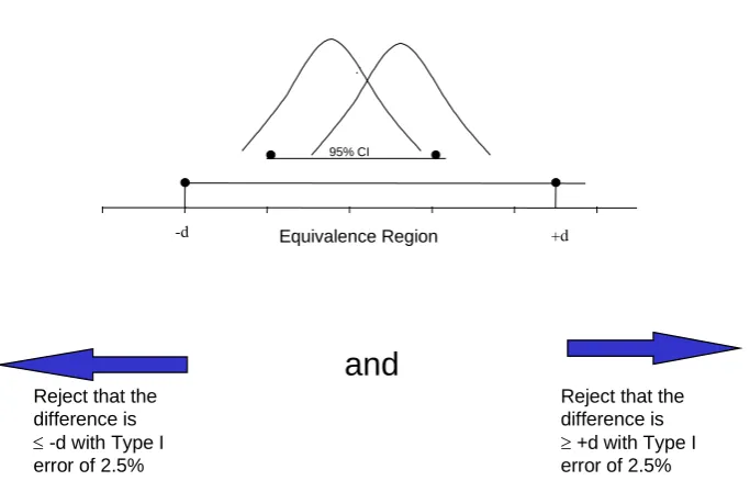
A common approach with equivalence trials to test each component of the null hypothesis

with a t test - called the Two One-Sided Test (TOST) procedure. In practice, this is

operationally the same as constructing a (1-2α)100% confidence interval for f

( )

equivalence is concluded provided that each end of the confidence interval falls completely

within the interval (−d,+d) [40]. This is because the (1-2α)100% confidence interval is

excluding two regions each of size α, each of which must simultaneously preclude (-d, +d).

Figure 1 highlights how equivalence can be demonstrated through confidence intervals and

Figure 2 demonstrated how confidence intervals are used to test the different hypotheses in

superiority and equivalence trials. The special case of bioequivalence is covered in Section 6.

ICH E10 [41] goes into some detail in the description of equivalence trials, and the related

non-inferiority trials (discussed in Section 4) whilst ICH E9 and E3 discuss the appropriate

analysis of such trials [3, 7].

In this section the sample size formulae will initially be derived

i) For the general case of inequality between treatments (i.e. f

( )

ii) Adopting the same notation and assumptions as in Section 2

iii) Under the assumption that the equivalence bounds –d and d are symmetric about zero

This section will then move on to the special case of no treatment difference replacing (i)

with:

i) For the special case of no mean difference (i.e. f

( )

3.1. General case

As with Section 2:

( )

f

S− µ

,

Hence, the

(

)

S Var Z

S−∆+ 1_−α ,

To declare equivalence the lower and upper confidence limit should be within ±d:

( )

Z

Thus, by extending the arguments for superiority trials, for the two one sided test procedure

(TOST) with this critical region there are two opportunities against an alternative to have a

Type II error for some chosen d and power (1-β)

Var(S) Var(S) -d -and Var(S) )

( 1 1 1

1−β₁ = −α ∆ −β₂ = −α

− +

∆ d Z Var S Z Z Z . (3.2)

where β₁ and β₂are the Type II errors associated with each one sided test from the TOST

procedure and β = β₁ +β₂. Hence,

( )

( )

β − − −

− − ∆ − = − ∆ − −

= 1 1 1

1 ₁ and ₂ Z

S Var d Z Z S Var d Z (3.3)

3.2. Special case of no treatment difference.

For the special case of no treatment difference ∆=0 can be entered into (3.1). Thus, with

the TOST procedure the Type II error for some chosen d and power (1-β) will come from

Var(S) Var(S) -d -and Var(S) )

( _{1 1 1}

1−β = −α −β = −α

−Z Var S Z Z Z

d .

Hence,

( )

β −

− /2 = − 1

1 Z S Var d Z , giving: 2 2 / 1 1 ) ( 2 ) ( β α − − + = Z Z d S

Var . (3.4)

3.3. Type I and setting the equivalence limit 3.3.1. Choice of Type I error

Strictly speaking when undertaking two simultaneous one tailed tests setting α=0.05 would

controversial issue. The convention for equivalence trials is to set the Type I error rate at

half of that which would be employed for a two sided test used in a superiority trial i.e.

α=0.025. That is, giving a Type I error rate of 2.5% [3]. However, setting the Type I error

rate for equivalence trials at half that for superiority trials could be considered to be

consistent. This is because although in a superiority trial one has a two sided 5%

significance level in practice for most trials in effect what one has is a one sided investigation

with a 2.5% level of significance. The reason for this is that one usually has an investigative

therapy and a control therapy and it is only statistical superiority of the investigative therapy

that is of interest.

Through the rest of the sections on equivalence and non-inferiority trials the assumption will

be that α=0.025 and that 95% confidence intervals will be used in the final statistical

analysis. This issue will be discussed again in the section on Bioequivalence.

3.3.2. Choice of Equivalence Limit

The discussion on equivalence limits in this section can also be generalised to non-inferiority

trials discussed in the proceeding section. As with the choice of the Type I error the setting

of the non-inferiority/equivalence limit is a controversial issue. The equivalence limit is

defined as the "largest difference that is clinically acceptable, so that a difference bigger than

this would matter in practice" [42]. This difference also cannot be "greater than the smallest

effect size that the active (control) drug would be reliably expected to have compared with

placebo in the setting of the planned trial" [41].

However, beyond this there has not much formal guidance. Jones, Jarvis, Lewis et al [40]

have recommended that the choice of limit be set at half the expected clinically meaningful

difference between the active control and placebo. There are no hard regulatory guidance

acceptable to have an equivalence limit "of one half or one third of the established superiority

of the comparator to placebo, especially if the new agent has safety or compliance

advantages"

The definition of the acceptable level of equivalence or non-inferiority is made therefore with

reference to some retrospective comparison to placebo [44, 45, 46]. In this context the

definition of the non-inferiority and equivalence limits should address steps of the form [45,

46].

1. One must be confident that the active control would have been different from placebo had

one been employed.

2. One should be able to determine that there is no clinically meaningful difference between

investigative treatment and the control.

3. Through comparing the investigative treatment to control one should indirectly be able to

determine that it is superior to placebo.

Steps 1. and 3. are important as there is a view that non-inferiority and equivalence trials

reward "failed" studies i.e. if one conducted a poor trial where it would not have been

possible to demonstrate the control to be superior to placebo then a poor investigative therapy

may slip through comparison to this control. However, Julious and Zariffa [2] point out that

this may not be the case as poor studies are poor for most objectives due to their higher

statistical variability.

In summary therefore one can infer that the clinical difference used for the limits of

equivalence and non-inferiority will be smaller than the difference used for placebo

controlled superiority trials. There is no generic definition for its setting – its definition will

3.4. Parallel group trials 3.4.1. General case.

For equivalence trials the sample size cannot be derived directly for the general case where

the expected true mean difference is not fixed to be zero. This is because the total Type II

error is the sum of the Type II errors associated with each one-tailed test.

As is the case with superiority trials Var(S) can be defined as :

( )

2 _{σ σ}

σ

r r S

Var = + = + . _(3.5)

From this (and the fact that β =β₁ +β₂), equation (3.3) can be used to derive the power

(and Type II error):

(

)

(

)

1 _{2 1}

2 1 2 2 −         − + + − Φ +         − + − − Φ =

− _{−α −α}

σ µ µ σ µ µ β Z r rn d Z r rn

d _{A A B A}

B

A _{. (3.6)}

To obtain the required sample size equation (3.6) until a sample size is reached which gives

the required power (Type II error ). For unknown variance equation (3.6) can be re-written

as:

(

)

(

)

1 _{2 1 , ( 1) 2}

2 2 ) 1 ( , 1 2 2 −         − + + − Φ +         − + − − Φ =

− _{− + −} A B A _{− n r+ −}

r n A B A A A t r rn d t r rn d α α _σ µ µ σ µ µ β .(3.7)

As with superiority trials it is best to use a non-central t-distribution to calculate the Type II

error and power. From a non-central t-distribution the power can be calculated using the

following formula [37, 47, 48]

(

)

(

)

Probt

1−β = −t_−αn_A r_{+ −} nA r+ − τ t_−αn_A r_{+ −} nA r+ − τ , (3.8)

where τ1and τ2are non centrality parameters defined as:

(

)

and

(

)

For quick calculations (and to provide an initial value for the sample size in the iterations), an

estimate of the sample size can be obtained from the following equation

(

)

(

)

2 1 1 2 ) ( ) 1 ( d r Z Z r n B A A − − + + = − − µ µ

σ _{β α}

. (3.9)

This provides reasonable approximations for the sample size when the mean difference is

greater than zero (µA −µB >0), and approaches d. For very quick calculations (for 90%

power and Type I error of 2.5%), the following formula can be used:

(

)

r n B A A 2 2 ) ( ) 1 ( 5 . 10 − − + = µ µ σ

, (3.10)

or for r=1:

(

)

2 ) ( 21 d n B A A − − = µ µ σ

. (3.11)

3.4.2. Special case of no treatment difference.

For the special case of no treatment difference (µA −µB =0), equation (3.5) can be

substituted into equation (3.4) to obtain a direct estimate of the sample size

(

)

σ ₋ + ₋

+

= . (3.12)

For unknown variance equation (3.12) can be as

2 2 2 ) 1 ( , 1 2 1 2 ) 1 ( rd t Z r n r n A A         + + ≥ − + −

−β α

σ

, (3.13)

Where nA is the smallest integer value to satisfy equation (3.12). Equation 3.13 can in turn

be rewritten to give power in terms of the sample size:

1 )

1 ( 2

1 _{1 , ( 1) 2}

2 2 −         − + Φ =

− A _{− n r+ −}

A t r n rd α σ

Similarly to equation (3.8), under the assumption of a non-central t-distribution, the power

can be derived from

(

)

Probt 2

1−β = −t1−α,n_A(r+1)−2 nA r+ − τ − , (3.15)

where τ is defined as

2 ) 1

( σ

τ

+ − =

r rd nA

.

For quick calculations (for 90% power and Type I error of 2.5%), the following formula can

be used:

r d

r

n_{A 2}

2 ) 1 (

13 +

= σ , (3.16)

or, for r=1,

2 2 26

d nA

σ

= . (3.17)

It is worth noting here the difference between equations 3.16 and 3.17 and those given earlier

equations 3.10 and 3.11. There is a difference in the coefficients (10.5 and 21 for equations

3.10 and 3.11 respectively and compared to 13 and 16 for equations 3.16 and 3.17) which is

due to the non-symmetric allocation of the Type II error if the population mean is non zero.

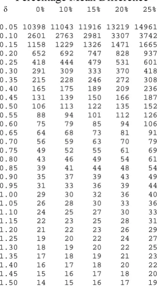
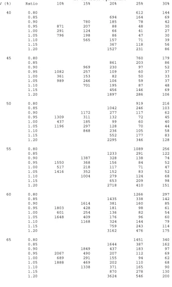
Table 3.1 gives sample sizes using equation 3.8 for various standardised equivalence limits

3.4.3. Worked example

3.4.3.1. Using the sample size tables

An investigator wishes to design a pain trial where the objective is to demonstrate

equivalence between two treatments. The largest clinically acceptable effect for which

equivalence can be declared is a change in visual analogue scale (VAS) assessed pain of

10mm (d). There is to be equal allocation between groups. The true mean difference

between the treatments is thought to be zero and the expected standard deviation in the

population in which the trial is to be undertaken is 50mm (σ ). Thus, the standardised

equivalence limits are ±δ =±d/σ =±10/50=±0.20. For the Type I and Type II errors

fixed at 2.5% and 10% respectively Table 3.1 gives a sample size of 651 patients in each arm

of the trial.

Suppose the true mean difference is thought to be 2mm. This equates to 20% of the

standardised equivalence limits and would inflate the sample size to 827 patients in each arm

of the trial.

3.4.3.2. Repeated using sample size software

To repeat the calculations in PASS one needs to select Means and then Equivalence-Means.

The dialogue box below details the entries required to repeat both calculations in the worked

example. One typographical issue to note is that PASS does not distinguish between

bioequivalence and equivalence trials which as will be highlighted Section 6 are two

difference concepts and so as a result PASS has as the heading in the output box

PASS gives a sample sizes respectively 651 and 827 respectively for the case of no treatment

difference and a treatment difference of 2mm. The same as table 3.1.

To repeat the calculations in nQuery one would need to click on File/New, for Goal tick

Means, Number of Groups tick Two and Analysis Method tick Equivalence. Then select

Two one-sided tests (TOST) for two group or cross-over. nQuery too gives the same answers

as table 3.1 for the two cases in the worked example.

3.5. Cross-over trials

The methodologies and assumptions for an equivalence trial with a cross-over design

are the same as those for parallel group trials . This subsection will therefore only go

3.5.1. General case.

The power (and Type II error) can be estimated from

(

)

(

)

1 _{2 1}

2 1 2 2 −         − + − Φ +         − − − Φ =

− _{−α −α}

σ µ µ σ µ µ

β d n Z d n Z

w B A w B A

. (3.17)

For unknown variance equation (3.17) can thus be re-written as

(

)

(

)

1 _{2 1 , 2}

2 2 , 1 2 2 −         − + − Φ +         − − − Φ =

− _{− − − n−}

w B A n w B A t n d t n d α α _σ µ µ σ µ µ

β , (3.18)

and under the assumption of a non-central t-distribution the power [Owen, Diletti et al, Chow

et al) the power can be estimated from

(

)

(

)

1−β = −t_−αn− n− τ t_−αn− n− τ , (3.19)

where τ₁and τ₂are defined as

(

)

A d n

σ µ µ

τ = − + and

(

)

2 2 2 ) ( w B

A d n

σ µ µ

τ = − − .

For quick calculations one could use:

(

)

(

)

2 1 1 2 ) ( 2 d Z Z n B A w − − + = − − µ µ

σ _{β α}

, (3.20)

for sample size estimation and for very quick calculations (for 90% power and Type I error of

2.5%), one can use the following formula:

(

)

2 ) ( 21 d n B A w − − = µ µ σ

3.5.2. Special case of no treatment difference.

For the special case of no treatment difference (µ_A −µ_B =0), a direct estimate of the sample

size can be estimated from

(

)

n= σw −β + −α , (3.22)

which, with unknown variance, can be re-written as

2 2 2 , 1 2 1 2 2 d t Z n n w       + = − −

−β α

σ

. (3.23)

Equation 3.23 can in turn be re-written in terms of power for a given sample size

1 2

2

1 2 1 , 2

2 −         − Φ =

− − n−

w t n d α σ

β , (3.24)

which in turn (under the assumption of a non-central t-distribution), can also be rewritten as:

(

)

2

1−β = −t_1−α,n−2 n− τ − , (3.25)

where τ is defined as

2 2 w d n

σ τ = − ,.

For quick calculations (for 90% power and Type I error of 2.5%), the following formula,

can be used:

2 2 26

d

n= σw _{. (3.26)}

The quick equations give reasonable estimates of the sample size, underestimating the

sample size by just one or two subjects, and thus provides reasonable initial values for

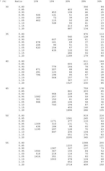
equations (3.19) and (3.25). Table 3.2 gives sample sizes using equation 3.19 for various

3.5.3 Worked example

3.5.3.1. Using the sample size tables

An investigator wishes to design a pain trial similar to that in Section 3.4.3.1. Again the

largest clinically acceptable effect for equivalence to be declared is a change in visual

analogue scale (VAS) assessed pain of 10mm (d) and the true mean difference between the

treatments is thought to be zero. The expected within-subject standard deviation in the trial

population is 20mm (σ_w). Thus, the standardised equivalence limits equate to

50 . 0 20 / 10

/ =± =±

± =

±δ d σ . For the Type I and Type II errors fixed at 2.5% and 10%,

respectively, Table 3.2 gives a total sample size of 106 patients in the trial.

If the true mean difference is thought to be 2mm, equating to 20% of the standardised

equivalence limits, the sample size would be inflated to a total of 135 patients in the trial.

3.5.3.2. Repeated using sample size software

To do the same sample size calculations in nQuery one would need to click on File/New, for

Goal tick Means, Number of Groups tick Two and Analysis Method tick Equivalence. Then

select Two one-sided tests (TOST) for two group or cross-over. For equivalence trials

nQuery does not use σ_d, as it does for superiority trials, or σ_w, as used in equation 3.9 but a

new variance σw 2, as described in the right hand dialogue box below under the heading

"Suggestion". One rational for using this variance is that nQuery does not give the total

sample size but the sample size per sequence (assuming one has two sequences AB and BA).

By using σ_w 2 for the variance estimate (and by giving the sample size per sequence) it

enables nQuery to use the same formula (equation 3.8), for sample size calculations for both

statistic in equation (3.8) will be correct for both cross-over and parallel group trials using

the nomenclature of sample size per sequence.

The dialogue box below gives the entries to repeat the sample size calculations in nQuery

For the equivalent sample sizes to those given earlier for no mean difference and a mean

difference of 2 nQuery gives a sample size per treatment sequence of 53 and 68 respectively

or 106 and 136 in total. Taking account of rounding nQuery gives the same results for the

total sample size as table 3.2. To do the same calculations in PASS one needs to select

Means and then Equivalence-Means. the dialogue box is the same as that in Section 3.4.3.2.

It is worth noting that for the variance PASS uses σ_w2 (and not σ_w2 2 as with nQuery) but

like nQuery it does give the sample size per sequence. PASS gives the same sample size per

sequence as nQuery.

There is an issue with the approach of nQuery and PASS in calculating the sample size per

sequence as this is assuming that one is investigating just 2 treatments in just 2 sequences

(BA and AB). If one was simultaneously investigating 3 treatments say one may have 6

sequences. Another issue is that even if just two treatments are being investigated one may

be applying a replicate design as described in Section 6.3.3 where again more than two

sequences may be being used. It is more optimal therefore to calculate the total sample size

and divide this by the number of sequences to get the sample size per sequence rather than

4. NON-INFERIORITY TRIALS

For certain trials the objective is not to demonstrate that two treatments are different or

equivalent but rather to demonstrate that a given treatment is clinically not inferior compared

to another. The null (H0) and alternative (H1) hypotheses for non-inferiority trials may take

the form:

H0: A given treatment is inferior with respect to the mean response.

H1: A given treatment is non-inferior with respect to the mean response.

As with equivalence trials these hypotheses are written in terms of a clinical difference, d,

which equates to the largest difference that is clinically acceptable [42]:

H0: µA −µB ≤−d .

H1: µA −µB >−d.

In the context of non-inferiority trials –d is know as the non-inferiority limit. Please see

discussion in section 3.3.2 as to its definition. ICH E3 and E9 go into detail on the analysis

of non-inferiority trials whilst ICH E10 discusses the definition of d [3, 7, 41].

In order to conclude non-inferiority, one needs to reject the null hypothesis. In terms of the

equivalence hypotheses in Section 3 this is equivalent to testing just one of the two

components of the TOST procedure. Thus, non-inferiority trials reduce to a simple one-sided

hypothesis and test. In practice, this is operationally the same as constructing a (1-2α)100%

confidence interval and concluding non-inferiority provided that the lower end of this

confidence interval is greater than –d.

Usually non-inferiority trials (like equivalence trials) compare the investigative therapy to an

active control. Statistically they could be considered a special case of equivalence trials.

However, operationally non-inferiority trials are more often conducted since it is only the

lower equivalence (now non-inferiority) limit that is usually of interest. For a non-inferiority

the study. Please see also the discussion on "as good as or better trials" for the context of

non-inferiority studies with superiority studies.

Figure 3 highlights how non-inferiority can be demonstrated through a confidence interval

and Figure 2 shows how confidence intervals are used to test the different hypotheses in

superiority, equivalence and non-inferiority trials.

Adopting the same notation and assumptions as in Section 3 but with f

( )

non-inferiority bound set at –d, the lower

(

)

S Var Z

S−∆− _1−α . (4.1)

To declare non-inferiority the lower end of the confidence interval should lie above –d:

( )

Z

S−∆− _1−α >− . (4.2)

For this critical region one therefore requires a

(

)

above –d i.e.:

Hence:

( )

1−β − −α

∆ + −

= Z

S Var

d

Z , (4.3)

giving:

(

)

2 1 1

2

) (

) (

β

α −

− +

∆ − =

Z Z

d S

Var . (4.4)

4.1. Parallel group trials

As with superiority and equivalence trials Var(S) can be defined as

( )

A r r S Var

n . 1 _σ2

+

= ,

(

)

(

)

2 1 1 2 ) ( ) 1 ( d r Z Z r n B A A − − + + = − − µ µ

σ _{β α}

. (4.5)

Re-writing equation (4.5) to give power for a give sample size results in:

(

)

− _−α

σ µ µ

β ₂ 2 ₁

) 1 ( ) ( 1 Z r rn d _A B A

. (4.6)

The equivalent formula to (4.6), in the case of unknown variance is

(

)

− _{2 1− , ( +1)−2}

2 ) 1 ( ) (

1 A B A _{n r}

A t r rn d α σ µ µ

β . (4.7)

As with the sections on equivalence and superiority trials when the population variance is

unknown it is best to calculate the power under the assumption of a non-central t-distribution

[37]:

(

)

β 1 Probt _α , ( 1) 2, 1− = − t_{1− ,n (r+1)−2} n_A r+ −

A , (4.8)

where τ is defined as

(

)

For quick calculations (for 90% power and Type I error of 2.5%), the following formula,

similar to equation (2.9) can be used:

(

)

r n B A A 2 2 ) ( ) 1 ( 5 . 10 − − + = µ µ σ

. (4.9)

In the case of r=1 (4.9) resolves to:

(

)

2 ) ( 21 d n B A A − − = µ µ σ

. (4.10)

Equations 4.9 and 4.10 are equivalent to equations 3.10 and 3.11 for the case of a non zero

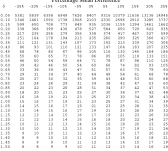
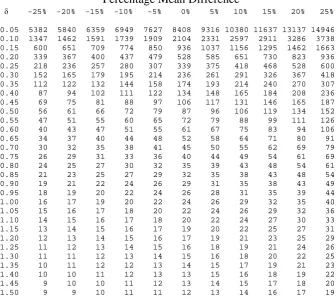
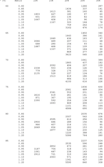
sample size, although with slight underestimation. Table 4.1 gives sample sizes using

equation 4.8 for various standardised non-inferiority limits (δ =d σ ) and standardised mean

differences assuming equal allocation between groups.

One important feature to highlight in tables 4.1 and 4.2 is the asymmetric effect on the sample

size of different values for the true mean difference. In equivalence trials as there are two

margins when one moves away from a zero mean difference - in any direction - the sample

size is inflated. However, in non-inferiority trials the sample size is inflated only if the true

mean difference moves towards the non-inferiority margin. If it is expected that the true mean

difference is in favour of the comparator regimen (compared to control) then the sample size

is significantly reduced.

The asymmetric effect of the mean difference on the sample size should be considered when

designing non-inferiority trials as even only a small expected mean difference in favour of the

comparator could have a marked effect on the sample size.

4.1.1. Worked example

4.1.1.1. Using the sample size tables

An investigator wishes to design an hypertension trial where the objective is to demonstrate

that one treatment (an investigative therapy) is non-inferior to another (a standard therapy).

As with the worked example in Section 3.2.3 the largest clinically acceptable effect to be

able to declare non-inferiority is a change in blood pressure of 10mmHg (d). The true mean

difference between the treatments is thought to be zero with an expected standard deviation

in the trial population of 40mmHg (σ ). There is to be equal allocation between groups.

Thus, the standardised non-inferiority limits equate to −δ =−d/σ =−10/40=−0.25. For

size of 338 patients in each arm of the trial. The quick formula (equation 4.10) gives 336

patients in each arm.

Suppose, though, that one believes that the investigative therapy is a little superior to the

standard such that the true mean difference is thought to be 2mmHg. This inflates the

distance one expects the mean to be away from the non-inferiority margin by 20% and as a

consequence reduces the sample size to required to 235 patients in each arm of the trial.

4.1.1.2. Repeated using sample size software

To do non-inferiority sample size calculations in nQuery one would need to click on

File/New, for Goal tick Means, Number of Groups tick Two and Analysis Method tick

Equivalence. Then click on Equivalence of Two Means.

Note that nQuery does not refer to these calculations as non inferiority but equivalence.

However, it is clear from the instructions and the definition of the null hypothesis given in

nQuery that the calculations are for a Non-inferiority trial (see the definition of the null