Simultaneous determination of time-dependent coefficients in the heat equation

promoting access to White Rose research papers

White Rose Research Online

Universities of Leeds, Sheffield and York

http://eprints.whiterose.ac.uk/

This is the Author's Accepted version of an article published in Computers and Mathematics with Applications

White Rose Research Online URL for this paper:

http://eprints.whiterose.ac.uk/id/eprint/78427

Published article:

Hussein, MS, Lesnic, D and Ivanchov, MI (2014)Simultaneous determination of time-dependent coefficients in the heat equation. Computers and Mathematics with Applications, 67 (5). 1065 - 1091. ISSN 0898-1221

Simultaneous determination of time-dependent

coefficients in the heat equation

M.S. Hussein1,2, D. Lesnic1 and M.I. Ivanchov3

1_{Department of Applied Mathematics, University of Leeds, Leeds LS2 9JT, UK}

2_{Department of Mathematics, College of Science, University of Baghdad, Al-jaderia,}

Bagh-dad, Iraq

3_{Faculty of Mechanics and Mathematics, Department of Differential Equations, Ivan}

Franko National University of Lviv, 1, Universytetska str., Lviv, 79000, Ukraine

E-mails: [email protected] (M.S. Hussein), [email protected] (D. Lesnic), [email protected] (M.I. Ivanchov).

Abstract

In this paper, the determination of time-dependent leading and lower-order thermal co-efficients is investigated. We consider the inverse and ill-posed nonlinear problems of simultaneous identification of a couple of these coefficients in the one-dimensional heat equation from Cauchy boundary data. Unique solvability theorems of these inverse prob-lems are supplied and, in one new case where they were not previously provided, are rigorously proved. However, since the problems are still ill-posed the solution needs to be regularized. Therefore, in order to obtain a stable solution, a regularized nonlinear least-squares objective function is minimized in order to retrieve the unknown coefficients. The stability of numerical results is investigated for several test examples with respect to different noise levels and for various regularization parameters. This study will be sig-nificant to researchers working on computational and mathematical methods for solving inverse coefficient identification problems with applications in heat transfer and porous media.

Keywords: Inverse problems; Thermal properties; Nonlinear optimization.

1

Introduction

Simultaneous determination of several unknown coefficients in parabolic partial differen-tial equations has been investigated in various studies in the past, see e.g. the monographs of Prilepko et al. [27] and Ivanchov [17]. In heat conduction for example, attention was paid to the unique solvability of one-dimensional inverse problems for the heat equation in the case when the unknown thermal coefficients are constant [4], time-dependent [15, 16], space-dependent [1], or temperature-dependent, [20, 23, 24]. In these papers, the authors investigated the existence and uniqueness of solution of the inverse problem, though no numerical method/solution was presented.

boundary conditions and measured heat flux as overdetermination condition was consid-ered. In [10], the author considered retrieving lower-order time-dependent coefficients using the Trace Type Functional approach, [5], which assumes that the governing partial differential equation is valid at the boundary. However, this approach does not seem so stable [11], and it has never been applied to inverse coefficient identification problems in which the unknown coefficients appear at the leading order in the heat operator.

In this paper, we investigate the inverse problems of simultaneous determination of time-dependent leading and lower-order thermal coefficients. The paper is organized as follows. In the next section, we give the mathematical formulations of three inverse problems for which the unique solvability theorems of [14, 15] are stated and, it one case, proved. The numerical finite-difference discretisation of the direct problem is described in Section 3, whilst Section 4 introduces the regularized nonlinear minimization used for solving in a stable manner the inverse problems under investigation. In Section 5, we provide numerical results and discussion. Finally, conclusions are presented in Section 6.

2

Mathematical Formulations of the Inverse

Prob-lems

Consider the linear one-dimensional parabolic equation with time-dependent coefficients

C(t)∂u

∂t(x, t) =K(t) ∂2_u

∂x2(x, t) +Q(t) ∂u

∂x(x, t), (x, t)∈(0, ℓ)×(0, T) =: Ω (1)

where, in heat conduction, u represents the temperature in a finite slab of length ℓ > 0 recorded over the time interval (0, T) with T > 0, C and K represent the heat capacity and thermal conductivity of the heat conductor, respectively,Q(t) = c(t)v(t) withcandv

representing the heat capacity and velocity of a fluid flowing through the heat conducting body, [2, 9]. The first term in the right-hand side of equation (1) represents the diffusion, whilst the second term, if v(t) is positive, represents the convection. A similar situation occurs in porous media, [7], where the properties are referred to as hydraulic rather than thermal as in heat transfer. For example, in the contaminant transport in groundwater the first term in the right-hand side of equation (1) represents the dispersion of contaminant as it moves through the porous medium, whilst the second term withv(t) negative describes the advection of contaminant which flows along with the bulk movement of groundwater.

The initial condition is

u(x,0) =ϕ(x), x∈[0, ℓ], (2)

and the boundary and over-determination conditions are

u(0, t) = µ1(t), u(ℓ, t) =µ2(t), t∈[0, T], (3)

−K(t)ux(0, t) = ν1(t), K(t)ux(ℓ, t) = ν2(t), t∈[0, T]. (4)

Conditions (3) and (4) represent the specification of the boundary temperature and heat flux, respectively. Together they represent the Cauchy data for the inverse coefficient identification problems (ICIP) which are described next.

2.1

Inverse Problem 1

Assuming that c(t)v(t) = 0, the inverse problem 1 (IP1) requires the simultaneous de-termination of the time-dependent thermal conductivity K(t) > 0, the heat capacity

C(t)>0 and the temperature u(x, t) satisfying the one-dimensional heat equation

C(t)∂u

∂t(x, t) =K(t) ∂2_u

∂x2(x, t), (x, t)∈Ω (5)

subject to the initial and boundary conditions (2)–(4).

For this IP1 we have the following existence and uniqueness of solution theorems, [15].

Theorem 1. (Existence) Suppose that:

1. ϕ ∈C2_{[0, ℓ] and µ}

i, νi ∈C1[0, T] for i= 1,2.

2. The consistency conditions are satisfied:

µ1(0) =ϕ(0), µ2(0) =ϕ(ℓ), −ν1(0)ϕ′(ℓ) =ν2(0)ϕ′(0), µ′₁(0)ϕ′′(ℓ) =µ′₂(0)ϕ′′(0).

3. The following conditions are satisfied:

ϕ′(x)≥0, x∈[0, ℓ], ϕ′′(x) +ϕ′′(ℓ−x)>0, x∈[0, ℓ/2),

ν₁2(t) +ν₂2(t)>0, µ′₂(t)−µ′₁(t)≥0, (1 +χ(t))µ′₁(t) + (1−χ(t))µ′₂(t)>0,

χ(t)>0, χ′(t)≥0, t∈[0, T],

(1 +χ(t))ϕ′′(x) + (1−χ(t))ϕ′′(ℓ−x)>0, x∈[0, ℓ/2], t∈[0, T],

ϕ′′(x)−ϕ′′(ℓ−x)≥0, or ϕ′′(x)−ϕ′′(ℓ−x)≤0, x∈[0, ℓ/2],

where χ(t) = _ν1ν2(₍t_t))+₋ν1_ν2(₍t_t)₎. Then, for a sufficiently small T > 0, the inverse problem (2)– (5) has at least one solution {C(t), K(t), u(x, t)}, where the functions C(t) and K(t) are continuous and positive on [0, T] and u(x, t) belongs to the class C2,1_(Ω)∩C1,0_(Ω).

Theorem 2. (Uniqueness)

Suppose that the following conditions are satisfied:

1. ϕ ∈C2_{[0, ℓ], µ}

i ∈C1[0, T] and νi ∈C[0, T] for i= 1,2;

2. ϕ′′(x) ≥ 0 for x ∈ [0, ℓ], ϕ′′(0) > 0, µ′₁(t) > 0, µ′₂(t) > 0, ν1(t) < 0, ν2(t) > 0 for t ∈[0, T].

If {Cj(t), Kj(t), uj(x, t)} for j = 1,2, are two solutions to the problem (2)–(5) such that

2.2

Inverse Problem 2

Assuming thatK(t)>0 is known, we now wish to determine the time-dependent heat ca-pacityC(t)>0, the convection/advection coefficientQ(t) and the temperatureu(x, t) sat-isfying equations (1)–(4). By dividing (1) withC(t) and denoting witha(t) :=K(t)/C(t) the thermal diffusivity andb(t) :=Q(t)/C(t), we obtain

∂u

∂t(x, t) =a(t) ∂2_u

∂x2(x, t) +b(t) ∂u

∂x(x, t), (x, t)∈Ω. (6)

For simplicity, since K(t)>0 is known we can divide with it in (4) and denote the right hand sides by

−ux(0, t) = ν1(t)/K(t) =:ν1(t), ux(ℓ, t) =ν2(t)/K(t) =:ν2(t), t∈[0, T]. (7)

For this inverse problem 2 (IP2), we have the existence and uniqueness of solution The-orems 3 and 4 below, [16]. These are actually given for the more general reaction-convection-diffusion equation with a source term, namely,

∂u

∂t(x, t) =a(t) ∂2u

∂x2(x, t) +b(t) ∂u

∂x(x, t) +d(x, t)u+f(x, t), (x, t)∈Ω, (8)

where d and f are some given functions representing the reaction rate and source term, respectively. The triplet (a(t), b(t), u(x, t)) is called a solution to the IP2 given by equa-tions (2), (3), (7) and (8) if it satisfies these equaequa-tions and it belongs to the class (Hγ/2_{[0, T])}2 _×H2+γ,1+γ/2_{(Ω) for some γ ∈ (0,1), and a(t) > 0 for all t ∈ [0, T]. For}

the definition of the H¨older space, as well as other spaces of functions involved, see [21].

Theorem 3. (Existence)

Suppose that the following conditions are satisfied:

1. ϕ ∈H2+γ[0, ℓ], µi, νi ∈H1+γ/2[0, T] for i= 1,2, and d, f, dx, fx∈Hγ,γ/2(Ω);

2. (µ′₁(t)−f(0, t)−d(0, t)µ1(t))ν2(t)+(µ′2(t)−f(ℓ, t)−d(ℓ, t)µ2(t))ν1(t)>0, ν1(t)≥0, ν2(t)≥0, ν2(t) +ν1(t)>0, t ∈[0, T], and ϕ′′(x)>0, x ∈[0, ℓ];

3. µ1(0) =ϕ(0), µ2(0) =ϕ(ℓ), −ν1(0) =ϕ′(0), and ν2(0) =ϕ′(ℓ).

Then the problem (2), (3), (7) and (8) has a (local) solution for x ∈[0, ℓ] and t ∈[0, t0],

where the time t0 ∈(0, T], is determined by the input data of the problem.

Theorem 4. (Uniqueness)

Suppose that the following condition is satisfied:

(µ′₁(t)−f(0, t)−d(0, t)µ1(t))ν2(t) + (µ′2(t)−f(ℓ, t)−d(ℓ, t)µ2(t))ν1(t)̸= 0, t∈[0, T].

2.3

Inverse Problem 3

For completeness, we consider the inverse problem 3 (IP3) which consists of determining the thermal conductivity K(t) > 0, the convection/advection coefficient Q(t) and the temperature u(x, t) satisfying equations (1)–(4), when the heat capacity C(t) is known. By dividing (1) with C(t) we obtain equation (6). Also, dividing (4) by the known

C(t)>0 we obtain

−a(t)ux(0, t) =

ν1(t)

C(t) =: ˜ν1(t), a(t)ux(ℓ, t) =

ν2(t)

C(t) =: ˜ν2(t), t ∈[0, T]. (9)

The following theorems give the unique solvability of solution of the IP3 given by equations (2), (3), (8) and (9).

Theorem 5. (Existence)

Suppose that the following assumptions hold: (A1)ϕ ∈C2+γ_{[0, ℓ], µ}

i ∈C1[0, T], ν˜i ∈C[0, T]f ori=1,2, d, f ∈Cγ,0(Ω), f orsome γ ∈ (0,1);

(A2) ϕ′′(x) >0, x∈ [0, ℓ], ν˜1(t) ≥0, ν˜2(t)≥ 0, ν˜2(t) + ˜ν1(t) >0, µ′1(t)−f(0, t)− d(0, t)µ1(t)>0, µ′2(t)−f(ℓ, t)−d(ℓ, t)µ2(t)>0, t ∈[0, T];

(A3) ϕ(0) =µ1(0), ϕ(ℓ) = µ2(0), −ν˜1(0)ϕ′(ℓ) = ˜ν2(0)ϕ′(0).

Then there exists t0 ∈ (0, T] such that the problem (2), (3), (8) and (9) has a (local)

solution (a(t), b(t), u(x, t))∈(C[0, t0])2×C2,1([0, ℓ]×[0, t0]) and a(t)>0, t∈[0, t0].

Proof. Putx= 0 and x=ℓ into equation (8) and use conditions (3) and (9) to obtain

µ′₁(t) =a(t)uxx(0, t)− ˜

ν1(t)b(t)

a(t) +d(0, t)µ1(t) +f(0, t),

µ′₂(t) =a(t)uxx(ℓ, t) + ˜

ν2(t)b(t)

a(t) +d(ℓ, t)µ2(t) +f(ℓ, t).

From this we deduce

a(t) =[(µ′₁(t)−f(0, t)−d(0, t)µ1(t))˜ν2(t) + (µ′2(t)−f(ℓ, t)−d(ℓ, t)µ2(t))˜ν1(t) ]

×(˜ν2(t)uxx(0, t) + ˜ν1(t)uxx(ℓ, t))−1, t∈[0, T], (10)

b(t) = a(t)[(µ′₂(t)−f(ℓ, t)−d(ℓ, t)µ2(t))uxx(0, t)−(µ′1(t)−f(0, t)−d(0, t)µ1(t))uxx(ℓ, t)

]

×(˜ν2(t)uxx(0, t) + ˜ν1(t)uxx(ℓ, t))−1, t∈[0, T]. (11) To find the solution of the direct problem (2), (3) and (8), we introduce a new unknown function

v(x, t) :=u(x, t)−ϕ(x)−µ1(t) +µ1(0)− x

ℓ(µ2(t)−µ2(0)−µ1(t) +µ1(0)). (12)

The functionv(x, t) satisfies the following problem:

vt=a(t)vxx+b(t)vx+d(x, t)v +f(x, t)−µ′1(t)− x ℓ(µ

′

2(t)−µ′1(t))

+a(t)ϕ′′(x) +b(t)

(

ϕ′(x) + 1

ℓ(µ2(t)−µ2(0)−µ1(t) +µ1(0)) )

+d(x, t)

(

ϕ(x) +µ1(t)−µ1(0) + x

ℓ(µ2(t)−µ2(0)−µ1(t) +µ1(0)) )

, (x, t)∈Ω, (13)

v(x,0) = 0, x∈[0, ℓ], (14)

The solution of problem (12)–(14) is given by the Green’s formula and using (12) we obtain

u(x, t) = ϕ(x) +µ1(t)−µ1(0) + x

ℓ(µ2(t)−µ2(0)−µ1(t) +µ1(0))

+ t ∫ 0 ℓ ∫ 0

G(x, t;ξ, τ)

[

f(ξ, τ)−µ′₁(τ)− ξ

ℓ(µ

′

2(τ)−µ′1(τ)) +a(τ)ϕ′′(ξ)

+b(τ)

(

ϕ′(ξ) + 1

ℓ(µ2(τ)−µ2(0)−µ1(τ) +µ1(0)) )

+d(ξ, τ)

(

ϕ(ξ) +µ1(τ)−µ1(0) + ξ

ℓ(µ2(τ)−µ2(0)−µ1(τ) +µ1(0)) )]

dξdτ, (x, t)∈Ω,

(16)

where G = G(x, t;ξ, τ) is the Green function for the equation Vt = a(t)Vxx +b(t)Vx +

d(x, t)V with Dirichlet boundary conditions.

Differentiating (16) twice with respect to x we obtain

uxx(x, t) =ϕ′′(x) + t ∫ 0 dτ ℓ ∫ 0

Gxx(x, t;ξ, τ)

[

f(ξ, τ)−µ′₁(τ)− ξ

ℓ(µ

′

2(τ)−µ′1(τ)) +a(τ)ϕ′′(ξ)

+b(τ)

(

ϕ′(ξ) + 1

ℓ(µ2(τ)−µ2(0)−µ1(τ) +µ1(0) )

+d(ξ, τ)

(

ϕ(ξ) +µ1(τ)−µ1(0)

+ξ

ℓ(µ2(τ)−µ2(0)−µ1(τ) +µ1(0)) )]

dξ, (x, t)∈Ω. (17)

It is known, [12], that the estimate

ℓ ∫ 0

Gxx(x, t;ξ, τ)F(ξ, τ)dξ

≤ (t−constτ)1−γ/2 (18)

is true if the function F(x, t) is continuous in Ω and verifies the H¨older condition with respect tox with the exponent γ.

As ϕ′′(x) > 0, x ∈ [0, ℓ], and ϕ ∈ C2+γ_{[0, ℓ] we have that there exits M}

0 > 0 such

that ϕ′′(x)≥M0 >0, x∈[0, ℓ]. Taking into account (18), we conclude that there exists

t0 ∈(0, T] such that the estimation

t ∫ 0 dτ ℓ ∫ 0

Gxx(x, t;ξ, τ)

[

f(ξ, τ)−µ′₁(τ)− ξ

ℓ(µ

′

2(τ)−µ′1(τ)) +a(τ)ϕ′′(ξ)

+b(τ)

(

ϕ′(ξ) + 1

ℓ(µ2(τ)−µ2(0)−µ1(τ) +µ1(0)) )

+d(ξ, τ)

(

ϕ(ξ) +µ1(τ)−µ1(0)

+ξ

ℓ(µ2(τ)−µ2(0)−µ1(τ) +µ1(0)) )]

dξ≤ 1

2M0, (x, t)∈[0, ℓ]×[0, t0] (19)

holds. Then

uxx(x, t)≥ 1

and the denominator in (10) and (11) may be estimated as follows:

˜

ν2(t)uxx(0, t) + ˜ν1(t)uxx(ℓ, t)≥ 1

2M0(˜ν2(t) + ˜ν1(t))≥M1 >0, t∈[0, t0], (21)

for someM1 >0. Applying this estimate to (10), we obtain

a(t)≤A1 <∞, t ∈[0, t0], (22)

where the constantA1 is defined by the input data.

Using the estimation (19) in (17), we obtain that

uxx(x, t)≤max

[0,ℓ]

ϕ′′(x) + 1

2M0 =:M2 <∞, (x, t)∈[0, ℓ]×[0, t0]. (23)

Taking into account (21)-(23), we deduce from (10) and (11) that

a(t)≥A0 >0, |b(t)| ≤B <∞, t∈[0, t0], (24)

where the constantsA0 and B are defined by the input data.

Now we can apply the Schauder fixed-point theorem to the system of equations (10) and (11). Let us rewrite this system in the form

ω =P ω,

whereω:= (a(t), b(t)) andP := (P1, P2).Here the operatorP1is defined by the right-hand

side of the equation (10) after substituting into it the expression of uxx from (17), and the operator P2 is defined by the right-hand side of the equation (11) after substituting into it the expressions of uxx and a(t) from (17) and (10), respectively. It is clear that the operator P maps the set N := {(a, u) : A0 ≤ a(t) ≤ A1,|b(t)| ≤ B} into itself. The

compactness of the operator P is established by the same way as in [16]. Consequently, there exists at least one fixed point of the operator P in N, that means the existence of solution (a(t), b(t)) to the system of equations (10) and (11). After this, the function

u(x, t) is determined by (16), and the proof is complete.

Theorem 6. (Uniqueness)

Suppose that the following assumptions hold: (A4) d∈Cγ,0_{(Ω), f orsome γ ∈(0,1);}

(A5) ˜ν1(t)≥0, ν˜2(t)≥0, ν˜2(t) + ˜ν1(t)>0, µ′1(t)−f(0, t)−d(0, t)µ1(t)>0, µ′2(t)− f(ℓ, t)−d(ℓ, t)µ2(t)>0, t∈[0, T].

Then the problem (2), (3), (8) and (9) can have at most one solution(a(t), b(t), u(x, t))∈ (C[0, T])2×C2+γ,1(Ω) such that a(t)>0, t∈[0, T].

Proof. Suppose that the problem (2), (3), (8) and (9) has two different solutions (ai(t), bi(t), ui(x, t)), i ∈ {1,2}. Denote a := a1 −a2, b := b1 −b2, u := u1 −u2. The

triplet of functions (a(t), b(t), u(x, t)) is a solution of the following problem:

ut=a1(t)uxx+b1(t)ux+d(x, t)u+a(t)u2xx(x, t) +b(t)u2x(x, t), (x, t)∈Ω, (25)

u(x,0) = 0, x∈[0, ℓ], (26)

u(0, t) = 0, u(l, t) = 0, t ∈[0, T], (27)

The solution of the problem (25)-(27) has the following form:

u(x, t) = t

∫

0

ℓ

∫

0

G(1)(x, t;ξ, τ)(a(τ)u2ξξ(ξ, τ) +b(τ)u2ξ(ξ, τ))dξdτ, (x, t)∈Ω, (29)

where G(1)_{(x, t;ξ, τ) is the Green function for the equation V}

t = a1(t)Vxx +b1(t)Vx +

d(x, t)V with Dirichlet boundary conditions. After puttingx= 0 andx=ℓinto equation (25) and using the conditions (28) we obtain the system of equations

      

(

u2xx(0, t) + ν1_a1˜ ₍(_tt)_)a2b1(₍t_t)₎

)

a(t)−_a2˜ν1(_(tt)₎b(t) = −a1(t)uxx(0, t), t∈[0, T],

(

u2xx(ℓ, t)−_a1ν2˜₍(_tt)_)a2b1(₍t_t)₎

)

a(t) + ν2_a2˜ (_(tt)₎b(t) =−a1(t)uxx(ℓ, t), t ∈[0, T].

Solving this system we obtain

a(t) = −a1(t)(˜ν2(t)uxx(0, t) + ˜ν1(t)uxx(ℓ, t)) ˜

ν2(t)u2xx(0, t) + ˜ν1(t)u2xx(ℓ, t)

, (30)

b(t) = a1(t)

[

−u2xx(0, t)uxx(ℓ, t) +u2xx(ℓ, t)uxx(0, t)− b1(t)

a1(t)a2(t) (

˜

ν1(t)uxx(ℓ, t)

+ ˜ν2(t)uxx(0, t)

)]

(˜ν2(t)u2xx(0, t) + ˜ν1(t)u2xx(ℓ, t))−1, t∈[0, T]. (31)

Let us verify that

˜

ν2(t)u2xx(0, t) + ˜ν1(t)u2xx(ℓ, t)̸= 0, t ∈[0, T]. (32)

As (a2(t), b2(t), u2(x, t)) is a solution to the problem (2), (3), (8) and (9) we have from (10) that

a2(t) =[(µ′₁(t)−f(0, t)−d(0, t)µ1(t))˜ν2(t) + (µ′₂(t)−f(ℓ, t)−d(ℓ, t)µ2(t))˜ν1(t)]

×(˜ν2(t)u2xx(0, t) + ˜ν1(t)u2xx(ℓ, t))−1, t∈[0, T].

Here a2(t) > 0, t ∈ [0, T] and (µ′1(t) − f(0, t) −d(0, t)µ1(t))˜ν2(t) + (µ′2(t) −f(ℓ, t) − d(ℓ, t)µ2(t))˜ν1(t) > 0, as a consequence of the assumption (A5). Hence, the inequality

(32) is true. It means that we have a system of homogeneous Volterra integral equations (30) and (31) whose kernels verify the estimate (18). It yields that a(t) ≡ 0, b(t) ≡ 0, t ∈ [0, T]. Then, from (29) we also obtain that u(x, t) ≡0,(x, t)∈ Ω, and the proof is complete.

3

Solution of Direct Problem

The discrete form of our problem is as follows. We divide the domain Ω = (0, ℓ)×(0, T) into M and N subintervals of equal step length h and k, where h = ℓ

M and k =

T

N,

respectively. So, the solution at the node (i, j) is ui,j :=u(xi, tj), where xi =ih,tj =jk, fori= 0, M,j = 0, N.

Considering the general partial differential equation

ut=F(x, t, u, ux, uxx), (33)

the Crank-Nicolson method is based on central finite-difference approximations for space and forward finite-difference approximations for time which gives second-order conver-gence rate. This method is equivalent to take average of forward and backward Euler schemes in time, hence equation (33) can approximated as:

ui,j+1−ui,j

k =

1

2(Fi,j+Fi,j+1), i= 1,(M −1), j = 0,(N −1), (34)

ui,0 =ϕ(xi), i= 0, M , (35)

u0,j =µ1(tj), j = 0, N , (36)

uM,j =µ2(tj), j = 0, N . (37)

For our problem, equation (8) can be discretised in the form of (34) as

−Aj+1ui−1,j+1+ (1−Bi,j+1)ui,j+1−Cj+1ui+1,j+1 =

−Ajui−1,j + (1 +Bi,j)ui,j−Cjui+1,j+

k

2(fi,j+1+fi,j) (38) fori= 1,(M−1), j = 0, N, where fi,j :=f(xi, tj)

Aj =

k

2h2a(tj)− k

4hb(tj), Bi,j =− k

h2a(tj) + k

2d(xi, tj), Cj =

k

2h2a(tj) + k

4hb(tj).

At each time step tj+1, for j = 0,(N −1), using the Dirichlet boundary conditions (3),

the above difference equation can be reformulated as a (M −1)×(M −1) linear system of equations of the form,

Lu=b

where

u = (u1,j+1, u2,j, ..., uM−1,j+1)tr, b= (b1, b2, ..., bM−1)tr.

and L=       

1−B0,j+1 −(Aj+1+Cj+1) 0 · · · 0 0 0

−Aj+1 1−B1,j+1 −Cj+1 · · · 0 0 0

..

. ... ... . .. ... ... ...

0 0 0 · · · −Aj+1 1−BM−2,j+1 −Cj+1

0 0 0 · · · 0 −(Aj+1+Cj+1) 1−BM−1,j+1       

b1 = (1 +B0,j)u0,j+ (Aj +Cj)u1,j−2h(Cj+1µ1(tj+1) +Cjµ1(tj)) +

k

2(f0,j+1+f0,j),

bi =Ajui−1,j + (1 +Bi,j)ui,j+Cjui+1,j+

k

2(fi,j+1+fi,j), i= 2,(M −2),

bM−1 = (Aj +Cj)uM−2,j+ (1 +BM−1,j)u0,j+ 2h(Aj+1µ2(tj+1) +Ajµ2(tj))

+ k

As an example, consider the direct problem (2), (3) and (8) withT =ℓ= 1 and

a(t) = 1 +t, b(t) = 1 + 2t, d(x, t) = x2+t2, ϕ(x) = (1−3x)2, µ1(t) = et,

µ2(t) = 4et, f(x, t) = (1−3x)2et−18(1 +t)et+ (6 + 12t)(1−3x)et

−(x2+t2)(1−3x)2et.

With this input data, the exact solution is given byu(x, t) = (1−3x)2_et_{, and the desired} heat fluxes (4), forK(t) = 1, are ν1(t) = 6et and ν2(t) = 12et.

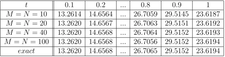
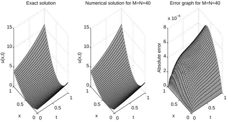
The numerical and exact solutions for u(x, t) are shown in Figure 1 and very good agreement is obtained. Tables 1 and 2 give the numerical heat fluxes in comparison with the exact ones. These have been calculated using the following O(h2_{) finite-difference}

approximations:

ux(0, tj) =

4u1,j−u2,j −3u0,j

2h , ux(ℓ, tj) =

4uM−1,j−uM−2,j−3uM,j

−2h , j = 1, N . (39)

From these tables it can be seen that the numerical results are in very good agreement with the exact solution and that a rapid monotonic increasing convergence is achieved.

Table 1: The exact and the numerical heat flux−ux(0, t) forM =N ∈ {10,20,40,100}, for the

direct problem.

t 0.1 0.2 ... 0.8 0.9 1

M =N = 10 -6.6309 -7.3282 ... -13.3529 -14.7573 -16.3093

M =N = 20 -6.6310 -7.3284 ... -13.3532 -14.7575 -16.3096

M =N = 40 -6.6310 -7.3284 ... -13.3532 -14.7576 -16.3097

M =N = 100 -6.6310 -7.3284 ... -13.3532 -14.7576 -16.3097

exact -6.6310 -7.3284 ... -13.3532 -14.7576 -16.3097

Table 2: The exact and the numerical heat flux ux(1, t) forM =N ∈ {10,20,40,100}, for the

direct problem.

t 0.1 0.2 ... 0.8 0.9 1

M =N = 10 13.2614 14.6564 ... 26.7059 29.5145 23.6187

M =N = 20 13.2620 14.6567 ... 26.7063 29.5151 23.6192

M =N = 40 13.2620 14.6568 ... 26.7064 29.5152 23.6193

M =N = 100 13.2620 14.6568 ... 26.7056 29.5152 23.6194

0 0.5 1 0 0.5 1 0 5 10 15 t Exact solution x u(x,t) 0 0.5 1 0 0.5 1 0 5 10 15 t Numerical solution for M=N=40

x u(x,t) 0 0.5 1 0 0.5 1 0 2 4 6 8

x 10−6

t Error graph for M=N=40

x

Absolute error

Figure 1: Exact and numerical solutions foru(x, t) and the absolute error for the direct problem (2), (3) and (8) obtained withM =N = 40.

4

Solution of Inverse Problems

In our inverse problems we wish to obtain simultaneously stable reconstructions of two un-known coefficients in equation (1), satisfying the initial and boundary conditions (2)–(4). The most common Tikhonov-type regularization approach is to impose the measured in-put data (4) in a penalised least-squares sense. This recasts into minimizing the following regularised (penalised) nonlinear objective functions.

For the IP1 given by equations (2)–(5) we minimize the functional

F1(K, a) := ∥ −K(t)ux(0, t)−ν1(t)∥2+∥K(t)ux(ℓ, t)−ν2(t)∥2

+β(∥K(t)∥2+∥a(t)∥2), (40)

where β ≥ 0 is a regularization parameter and the norm ∥ · ∥ is usually taken as the

L2_{[0, T] norm.}

For the IP2 given by equations (2), (3), (7) and (8) we minimize the functional

F2(a, b) :=∥ −ux(0, t)−ν1(t)∥2+∥ux(ℓ, t)−ν2(t)∥2

+β(∥a(t)∥2+∥b(t)∥2). (41)

For the IP3 given by equations (2)–(4) and (8) we minimize the functional

F3(K, b) := ∥ −K(t)ux(0, t)−ν1(t)∥2+∥K(t)ux(ℓ, t)−ν2(t)∥2

+β(∥K(t)∥2+∥b(t)∥2). (42)

The discretisations of (40)–(42) are:

F1(K, a) =

N

∑

j=0

[−K(tj)ux(0, tj)−ν1(tj)]2+ N

∑

j=0

[K(tj)ux(ℓ, tj)−ν2(tj)]2

+β ( _N

∑

j=0

K2(tj) + N

∑

j=0

a2(tj)

)

, (43)

F2(a, b) = N

∑

j=0

[−ux(0, tj)−ν1(tj)]2+ N

∑

j=0

[ux(ℓ, tj)−ν2(tj)]2

+β ( _N

∑

j=0

a2(tj) + N

∑

j=0

b2(tj)

)

, (44)

F3(K, b) =

N

∑

j=0

[−K(tj)ux(0, tj)−ν1(tj)]2+ N

∑

j=0

[K(tj)ux(ℓ, tj)−ν2(tj)]2

+β ( _N

∑

j=0

K2(tj) + N

∑

j=0

b2(tj)

)

, (45)

respectively.

It is worth mentioning that at the first time step, i.e. j = 0, the above equations (43)–(45) need to calculate the derivatives ux(0,0) and ux(ℓ,0) which are obtained from the initial condition (2), using (39) as:

ux(0,0) =

4ϕ1−ϕ2−3ϕ0

2h , ux(ℓ,0) =

4ϕM−1−ϕM−2−3ϕM

−2h , (46)

whereϕi =ϕ(xi) fori= 0, M.

If there is noise in the measured data (4), we replaceν1(tj) andν2(tj) in (43) and (45) by the noisy perturbations

ν₁ϵ1(tj) =ν1(tj) +ϵ1j, ν2ϵ2(tj) =ν2(tj) +ϵ2j, j = 0, N , (47)

where ϵ1j and ϵ2j are random variables generated from a Gaussian normal distribution with mean zero and standard deviationsσ1 and σ2, respectively, given by

σ1 =p× max

t∈[0,T]|ν1(t)|, σ2 =p×tmax∈[0,T]|ν2(t)|, (48)

where p represents the percentage of noise. We use the MATLAB function normrnd to generate the random variablesϵ1 and ϵ2 as follows:

ϵ1 =normrnd(0, σ1, N+ 1), ϵ2 = normrnd(0, σ2, N + 1). (49)

Note that via (7) we replace ν1 and ν2 in (44) by the noisy perturbations

4.1

Minimization Algorithms

Nevertheless, finding a global minimizer (even only approximately) to nonlinear (least-squares) problems is not an easy task. Numerical experience shows that the objective function which is, in general, non-convex has usually multiple local minima in which a descent method tends to get stuck if the underlying problem is ill-posed. Furthermore, the determination of an appropriate regularization parameterβ requires additional com-putational effort.

In this section, we give brief description of the routines f minconand lsqnonlinfrom the MATLAB Optimization Toolbox [25, 26] that we have employed for the constrained nonlinear minimization of the functionals defined by equations (40)–(42). These routines are based on interior trust region methods for nonlinear minimization, [3, 6].

The above routines attempt to find a minimum of a scalar objective function of several variables, starting from a initial guess, subject to simple bounds on the variables. In all examples of the next section, the initial guess was K0 _{= 1, a}0 _{= 1, b}0 _{= 1 and the}

lower and upper bounds were taken as LB(K) = LB(a) = 10−10, LB(b) = −103, and

U B(K) =U B(a) = U B(b) = 103_.

Apart from the initial guess, and the upper and lower bounds the routines also require the user to input some parameters such as:

• Number of variables M =N = 40.

• Maximum number of iterations = (102÷₁₀5₎×_{(number of variables).}

• Maximum number of objective function evaluations = (103÷107)×(number of variables).

• x Tolerance (xTol) = 10−10.

• Function Tolerance (FunTol) = 10−10_.

• Nonlinear constraint tolerance = 10−6_.

It is also worth noting that the user does not need to supply the gradient of the objective function which is minimized, as this is calculated internally within the routines using finite differences. Further, the Broyden, Fletcher, Goldfarb and Shanno (BFGS) technique is used to compute the Hessian matrix.

We finally mention that we have also used a combination between a generalized pattern search algorithm for the poll method and a genetic algorithm for the search method, both of them from the MATLAB Global Optimization Toolbox. In comparison with the previ-ously described interior-point algorithms the results were not significantly improved, but instead the computational time increased beyond purpose. For this reason, the numerical results obtained using this latter combined method are omitted.

5

Numerical Results and Discussion

We employ f mincon for IP1 and lsqnonlin for IP2 and IP3, for the minimization of the functionals (40)–(42). The other computational details have already been given in Subsection 4.1. We have also calculated the relative root mean square error (rrmse) to analyse the error between the exact and estimated coefficients, defined as,

rrmse(K(t)) =

v u u t 1

N + 1 N

∑

j=0

(

Knumerical(tj)−Kexact(tj)

Kexact(tj)

)2

, (51)

and similar expressions exist fora(t),b(t) and C(t).

One of the main difficulty when we solve inverse and ill-posed problems is how to choose an appropriate regularization parameter β which must compromise between accuracy and stability. Nevertheless, one can use techniques such as the L-curve method [13] or, Morozov’s discrepancy principle [22] to find such a parameter, but in our work we have used trial and error. As mentioned in [8], the regularization parameter β is selected based on experience by first choosing a small value and gradually increasing it until any numerical oscillations in the unknown coefficient are removed.

5.1

Example 1 for IP1

We first consider the problem IP1 given by equations (2)–(5), with unknown coefficients

C(t) andK(t), and we solve this inverse problem with the following input data:

ϕ(x) = (1 +x)2, µ1(t) = t2+t+ 1, µ2(t) =t2+t+ 4, ν1(t) = −(1 +t)(1 + 2t), ν2(t) = 2(1 +t)(1 + 2t),

forx∈(0, ℓ= 1) and t ∈(0, T = 1). The exact solution is given by

u(x, t) = (1 +x)2+t2+t, C(t) = 1 +t, K(t) = (1 +t)

( t+ 1

2

)

. (52)

We also have thata(t) = t+1₂, and one can easily check that the conditions of Theorems 1 and 2 are satisfied such that we know beforehand for sure that the solution to the IP1 exits and is unique.

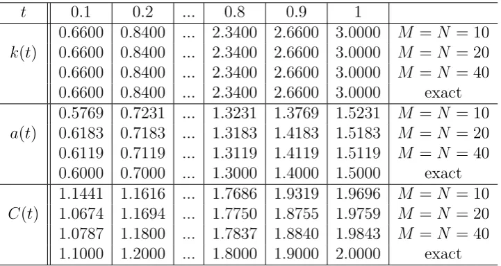
Table 3: The exact and the numerical coefficients for M = N ∈ {10,20,40}, for the IP1 of Example 1 and without noise.

t 0.1 0.2 ... 0.8 0.9 1

k(t)

0.6600 0.8400 ... 2.3400 2.6600 3.0000 M =N = 10 0.6600 0.8400 ... 2.3400 2.6600 3.0000 M =N = 20 0.6600 0.8400 ... 2.3400 2.6600 3.0000 M =N = 40 0.6600 0.8400 ... 2.3400 2.6600 3.0000 exact

a(t)

0.5769 0.7231 ... 1.3231 1.3769 1.5231 M =N = 10 0.6183 0.7183 ... 1.3183 1.4183 1.5183 M =N = 20 0.6119 0.7119 ... 1.3119 1.4119 1.5119 M =N = 40 0.6000 0.7000 ... 1.3000 1.4000 1.5000 exact

C(t)

1.1441 1.1616 ... 1.7686 1.9319 1.9696 M =N = 10 1.0674 1.1694 ... 1.7750 1.8755 1.9759 M =N = 20 1.0787 1.1800 ... 1.7837 1.8840 1.9843 M =N = 40 1.1000 1.2000 ... 1.8000 1.9000 2.0000 exact

In Figure 2, we present the regularized objective function (40) forp= 0 (no noise) and

p= 1% noise included in input data ν1(t) and ν2(t) for several regularization parameters β∈ {0,10−3_,10−2_,10−1_{}. From this figure it can be seen that convergence is achieved in a}

relatively small number of iterations. Also, it takes a slightly larger number of iterations when p = 1% noise contaminates the input data than when this data is errorless, i.e.

p= 0.

0 50 100 150 200 250

10−15 10−10 10−5 100 105

Number of Iterations

Regularised objective function

β=10−1

β=10−2

β=10−3

β=0

Figure 2: Regularised objective function (40), for Example 1 without noise (-×-) and with

p= 1% noise (—).

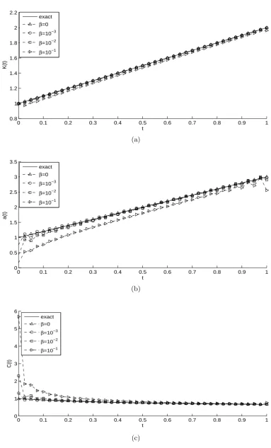
the identified coefficientsK(t),a(t) and C(t) which are convergent to their exact values. In the case β = 10−1 _{we observe that the graphs of the identified coefficients slightly}

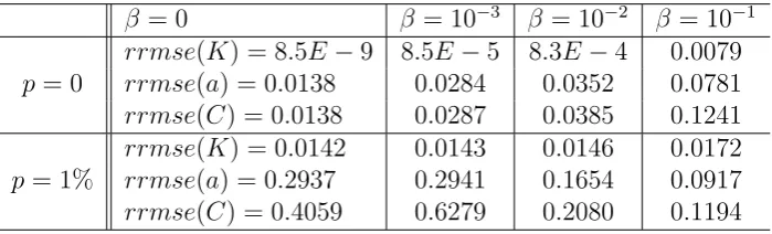
depart from the exact ones because we have added too much unwanted regularization to the objective function (40). In Figure 4 and Table 4 we present the retrieved coefficients and theirrrmsevalues, respectively, whenp= 1% noise is included in the input dataν1(t)

and ν2(t). It can be seen that the numerical retrieval of the thermal conductivity K(t)

is accurate; however, unstable results are obtained for a(t) and C(t) if no regularization, i.e. β = 0, is employed, or even if β is too small such as 10−3_{. Clearly, one can observe}

the effect of the regularization parameter β > 0 in decreasing the oscillatory unstable behaviour of the retrieved coefficients. Overall, the numerical results obtained with β = 10−1 _{seem the most stable and accurate.}

Table 4: The rrmsevalues for estimated coefficients in Example 1.

β = 0 β = 10−3 _{β = 10}−2 _{β = 10}−1

p= 0

rrmse(K) = 8.5E−9 8.5E−5 8.3E−4 0.0079

rrmse(a) = 0.0138 0.0284 0.0352 0.0781

rrmse(C) = 0.0138 0.0287 0.0385 0.1241

p= 1%

rrmse(K) = 0.0142 0.0143 0.0146 0.0172

rrmse(a) = 0.2937 0.2941 0.1654 0.0917

0 0.1 0.2 0.3 0.4 0.5 0.6 0.7 0.8 0.9 1 0

0.5 1 1.5 2 2.5 3

t

K(t)

exact

β=0

β=10−3

β=10−2

β=10−1

(a)

0 0.1 0.2 0.3 0.4 0.5 0.6 0.7 0.8 0.9 1

0.2 0.4 0.6 0.8 1 1.2 1.4 1.6

t

a(t)

exact

β=0

β=10−3

β=10−2

β=10−1

(b)

0 0.1 0.2 0.3 0.4 0.5 0.6 0.7 0.8 0.9 1 0.8

1 1.2 1.4 1.6 1.8 2 2.2 2.4

t

C(t)

exact

β=0

β=10−3

β=10−2

β=10−1

(c)

0 0.1 0.2 0.3 0.4 0.5 0.6 0.7 0.8 0.9 1 0

0.5 1 1.5 2 2.5 3 3.5

t

K(t)

exact

β=0

β=10−3

β=10−2

β=10−1

(a)

0 0.1 0.2 0.3 0.4 0.5 0.6 0.7 0.8 0.9 1 0

0.5 1 1.5 2

t

a(t)

exact

β=0

β=10−3

β=10−2

β=10−1

(b)

0 0.1 0.2 0.3 0.4 0.5 0.6 0.7 0.8 0.9 1

0.5 1 1.5 2 2.5 3 3.5 4 4.5 5

t

C(t)

exact

β=0

β=10−3

β=10−2

β=10−1

(c)

5.2

Example 2 for IP1

We next consider an example from [15] in which the input data satisfy the conditions of existence of solution of Theorem 1,

ϕ(x) = x

4

12 + 2x−4, µ1(t) = t

4_{+ 2t}3_+t2_{−4, µ}

2(t) =t4+ 2t3+ 2t2 +t−

23 12,

ν1(t) =−2t−2, ν2(t) = (t+ 1) (

2t2+ 2t+ 7 3

) ,

for x ∈ (0, ℓ = 1) and t ∈ (0, T = 1). However, the conditions of uniqueness of solution of Theorem 2 are all satisfied, but for the condition ϕ′′(0)>0 which is not satisfied. One can simply check by direct substitution that the solution

u(x, t) = t4+ 2t3+t2(x2+ 1) +tx2+ x

4

12+ 2x−4,

C(t) = 1 +t

1 + 2t, K(t) = 1 +t. (53)

satisfies the inverse problem (2)–(5). We also have thata(t) = 1 + 2t.

Figure 5 illustrates the objective function (40), as a function of the number of iterations for p = 0 (no noise) and p = 1% noise included in the input data ν1(t) and ν2(t). It is interesting to remark that forβ small such as 0 to 10−3 _{the convergence is non-monotonic}

with respect to the number of iterations. Also, the unregularized (β = 0) objective function reduces rather non-smoothly to reach a stationary value of O(10−7) for p = 0 and O(10−4_{) for p= 1%, whilst the curves obtained for β >0 reach rapidly a stationary}

plateau.

0 50 100 150 200 250 300 350 400 10−8

10−6 10−4 10−2 100 102 104

Number of Iterations

Regularised objective function

β=10−1

β=10−3

β=10−2

β=0

Figure 5: Regularised objective function (40), for Example 2 without noise (-×-) and with

0 0.1 0.2 0.3 0.4 0.5 0.6 0.7 0.8 0.9 1 0.8

1 1.2 1.4 1.6 1.8 2 2.2

t

K(t)

exact

β=0

β=10−3

β=10−2

β=10−1

(a)

0 0.1 0.2 0.3 0.4 0.5 0.6 0.7 0.8 0.9 1

0 0.5 1 1.5 2 2.5 3 3.5

t

a(t)

exact

β=0

β=10−3

β=10−2

β=10−1

(b)

0 0.1 0.2 0.3 0.4 0.5 0.6 0.7 0.8 0.9 1

0 1 2 3 4 5 6

t

C(t)

exact

β=0

β=10−3

β=10−2

β=10−1

(c)

0 0.1 0.2 0.3 0.4 0.5 0.6 0.7 0.8 0.9 1 0.8

1 1.2 1.4 1.6 1.8 2 2.2

t

K(t)

exact

β=0

β=10−3

β=10−2

β=10−1

(a)

0 0.1 0.2 0.3 0.4 0.5 0.6 0.7 0.8 0.9 1

0 0.5 1 1.5 2 2.5 3 3.5

t

a(t)

exact

β=0

β=10−3

β=10−2

β=10−1

(b)

0 0.1 0.2 0.3 0.4 0.5 0.6 0.7 0.8 0.9 1

0 1 2 3 4 5 6

t

C(t)

exact

β=0

β=10−3

β=10−2

β=10−1

(c)

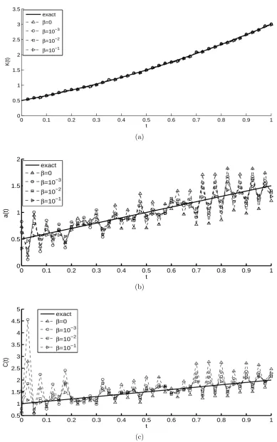
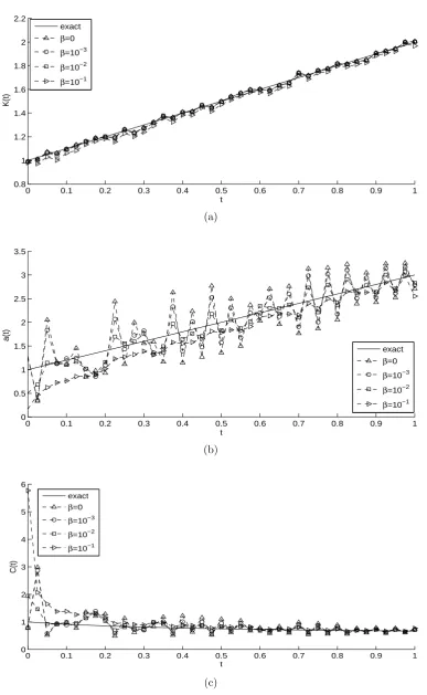
Figures 6, 7 and Table 5 for Example 2 represent the same quantities as Figures 3, 4 and Table 4 for Example 1, and the same conclusions can be drawn. We also mention that the numerical results obtained with β= 10−2 _{seem the most stable and accurate for} p= 1% noisy data.

Table 5: The rrmsevalues for estimated coefficients in Example 2.

β = 0 β = 10−3 _{β = 10}−2 _{β = 10}−1

p= 0

rrmse(K) = 5.6E−5 6.8E−4 0.0039 0.0223

rrmse(a) = 0.0078 0.0449 0.1000 0.2239

rrmse(C) = 0.0078 0.0552 0.2095 0.7778

p= 1%

rrmse(K) = 0.0123 0.0125 0.0146 0.0276

rrmse(a) = 0.3066 0.2301 0.1441 0.2321

rrmse(C) = 0.4350 0.3677 0.2135 0.7993

5.3

Example 3 for IP1

Finally, for IP1, we consider the case of a non-smooth coefficient and more complicated input data given by

ϕ(x) = x

2_+x

2 −

1 4,

µ1(t) =

{ 3t−t2

2 − 1

4 if t ∈[0, 1 2]

t+t2

2 if t ∈[ 1 2,1]

, µ2(t) =

{ 3t−t2

2 + 3

4 if t ∈[0, 1 2]

t+t2

2 + 1 if t ∈[ 1 2,1]

,

ν1(t) =−

1 2

(

1 +t− 1

2

), ν2(t) =

3 2

(

1 +t−1

2

),

for x∈ (0, ℓ = 1) and t ∈ (0, T = 1). One can remark that the conditions of Theorem 2 which ensure the uniqueness of solution are satisfied. The exact solution is given by

u(x, t) = x+x

2

2 +

{ 3t−t2

2 − 1

4 if t∈[0, 1 2]

t+t2

2 if t∈[ 1 2,1]

, C(t) = 1, K(t) = 1 +t− 1

2

. (54)

0 20 40 60 80 100 120 140 160 180 10−15

10−10 10−5 100 105

Number of Iterations

Objective function

0 0.1 0.2 0.3 0.4 0.5 0.6 0.7 0.8 0.9 1 0.9

1 1.1 1.2 1.3 1.4 1.5

t

K(t)

exact

final iteration 166 (p=0)

(a)

0 0.1 0.2 0.3 0.4 0.5 0.6 0.7 0.8 0.9 1

0.9 1 1.1 1.2 1.3 1.4 1.5

t

a(t)

exact

final iteration 166 (p=0)

(b)

0 0.1 0.2 0.3 0.4 0.5 0.6 0.7 0.8 0.9 1

0.98 0.985 0.99 0.995 1 1.005 1.01 1.015 1.02

t

C(t)

exact

final iteration 166 (p=0)

(c)

We next include noisep∈ {1%, 2%} in the input fluxesν1(t) andν2(t), as in (47). In

Figure 10, we can see that the regularized objective function becomes a smooth decreasing curve and the convergence is achieved in a relatively small number of iterations, as β

increases from 10−3 to 10−1. The numerical results forK(t),a(t) and C(t) whenp= 1% and p= 2% are presented in Figures 11 and 12, respectively. Further, numerical outputs such as the number of iterations and function evaluations, as well as the final value of the converged objective function and the rrmse values of the estimated coefficients are provided in Table 6. From these figures and table it can be seen that stable and reasonable accurate numerical results are obtained for β = 10−3 _{when p = 1%, and} β= 10−2 when p= 2% noise. The results forβ = 10−1 depart from the exact solution as too much regularization has been imposed, whilst the results forβ = 0 seem only slightly unstable. In fact from all examples presented in this section, see Tables 4–6, it seems that the retrieval of the thermal conductivity coefficientK(t) is stable even if we do not use regularization and we may as well penalise only the thermal diffusivity β∥a(t)∥2 _in

the last term of (40). Another reason for this stability of solution in theK(t)-component might be that K(t) appears explicitly in the nonlinear objective function (40). On the other hand the retrieval of the thermal diffusivitya(t) (and hence the heat capacityC(t)) does require some regularization to be enforced in order to ensure stability.

0 50 100 150 200 250 300

10−8 10−6 10−4 10−2 100 102

Number of Iterations

Regularized objective function

β=0

β=10−1

β=10−2

β=10−3

Figure 10: Regularized objective function (40), for Example 3 with p = 1% (—) and p = 2%

Table 6: Number of iterations, number of function evaluations, value of regularized objective function (40) at final iteration andrrmse values for estimated coefficients, for Example 3.

Noise level β = 0 β = 10−3 _{β = 10}−2 _{β = 10}−1

p= 1%

No. of iterations 181 205 190 93

No. of function evaluations 15035 17120 16105 7889

Function value 6.9E−7 0.1308 1.2778 11.03

rrmse(K) 0.0090 0.0094 0.0143 0.0842

rrmse(a) 0.0867 0.0619 0.0647 0.2232

rrmse(C) 0.0899 0.0668 0.0740 0.3045

p= 2%

No. of iterations 205 280 144 70

No. of function evaluations 17047 23563 12210 5919

Function value 2.7E−6 0.1316 1.2789 11.02

rrmse(K) 0.0181 0.0186 0.0221 0.0860

rrmse(a) 0.1710 0.1130 0.0794 0.2248

0 0.1 0.2 0.3 0.4 0.5 0.6 0.7 0.8 0.9 1 0.9

1 1.1 1.2 1.3 1.4 1.5 1.6

t

K(t)

exact

β=0

β=10−3

β=10−2

β=10−1

(a)

0 0.1 0.2 0.3 0.4 0.5 0.6 0.7 0.8 0.9 1

0.4 0.6 0.8 1 1.2 1.4 1.6 1.8 2

t

a(t)

exact

β=0

β=10−3

β=10−2

β=10−1

(b)

0 0.1 0.2 0.3 0.4 0.5 0.6 0.7 0.8 0.9 1

0.6 0.8 1 1.2 1.4 1.6 1.8 2 2.2 2.4 2.6

t

C(t)

exact

β=0

β=10−3

β=10−2

β=10−1

(c)

0 0.1 0.2 0.3 0.4 0.5 0.6 0.7 0.8 0.9 1 0.9

1 1.1 1.2 1.3 1.4 1.5 1.6

t

K(t)

exact

β=0

β=10−3

β=10−2

β=10−1

(a)

0 0.1 0.2 0.3 0.4 0.5 0.6 0.7 0.8 0.9 1

0.5 1 1.5 2

t

a(t)

exact

β=0

β=10−3

β=10−2

β=10−1

(b)

0 0.1 0.2 0.3 0.4 0.5 0.6 0.7 0.8 0.9 1

0.5 1 1.5 2 2.5 3

t

C(t)

exact

β=0

β=10−3

β=10−2

β=10−1

(c)

5.4

Example 4 for IP2

Consider now the IP2 given by equations (2), (3), (7) and (8) with unknown coefficients

a(t) and b(t), and solve this inverse problem with the following input data:

ϕ(x) =e−x+x2, µ1(t) =et, µ2(t) = (e−1 + 1)et, ν1(t) =et, ν2(t) = (2−e−1)et,

f(x, t) =et((1 +t)e−x+x2−2(1 +t)−2x(1 + 2t)), d(x, t) = 0,

forx∈(0, ℓ= 1) andt ∈(0, T = 1). One can easily check that the condition of Theorem 4 which ensures the uniqueness of solution is satisfied. The exact solution to this inverse problem is given by

a(t) = 1 +t, b(t) = 1 + 2t, u(x, t) = (e−x+x2)et. (55)

Consider first the case where there is no noise in the input data (7). The objective function (41), as a function of the number of iterations, is shown in Figure 13. From this figure it can be seen that the convergence is achieved rapidly in a few iterations. The objective function (41) decreases rapidly and takes a stationary value ofO(10−8_{) in about}

6 iterations. The numerical results for the corresponding coefficients a(t) and b(t) are presented in Figure 14. From this figure it can be seen that the retrieved coefficients are in very good agreement with the exact ones.

Next, we add p = 1% noise to the heat fluxes ν1 and ν2, as in equation (50) via

(47). The regularized objective function (41) is plotted, as a function of the number of iterations, in Figure 15 and convergence is rapidly achieved. Figure 16 presents the graphs of the recovered coefficients and further results are reported in Table 7. From this figure one can observe, as expected, that whenβ = 0 we obtain unstable and inaccurate solutions because the problem is ill-posed and sensitive to noise. So, regularization is needed in order to stabilise the solution. From all regularization parameters that were selected we deduce that β = 10−2 gives a stable and reasonable accurate approximation for the coefficients a(t) and b(t).

0 1 2 3 4 5 6

10−8 10−6 10−4 10−2 100 102 104

Number of Iterations

Objective function

0 0.1 0.2 0.3 0.4 0.5 0.6 0.7 0.8 0.9 1 0.8

1 1.2 1.4 1.6 1.8 2 2.2

t

a(t)

Exact Iteration 2 Iteration 3 Iteration 6

(a)

0 0.1 0.2 0.3 0.4 0.5 0.6 0.7 0.8 0.9 1

0.5 1 1.5 2 2.5 3

t

b(t)

exact Iteration 2 Iteration 3 Iteration 6

(b)

Figure 14: (a) Coefficient a(t), and (b) Coefficient b(t), for Example 4 with no noise and no regularization.

0 5 10 15 20 25 30

10−6 10−4 10−2 100 102 104

Number of Iterations

Regylarized objective function

β=0 β=10−3 β=10−2 β=10−1

0 0.1 0.2 0.3 0.4 0.5 0.6 0.7 0.8 0.9 1 0.8

1 1.2 1.4 1.6 1.8 2 2.2

t

a(t)

exact β=0 β=10−3 β=10−2 β=10−1

(a)

0 0.1 0.2 0.3 0.4 0.5 0.6 0.7 0.8 0.9 1

0 0.5 1 1.5 2 2.5 3 3.5

t

b(t)

exact β=0 β=10−3 β=10−2 β=10−1

(b)

Figure 16: (b) Coefficient a(t), and (b) Coefficientb(t), for Example 4 with p= 1% noise and regularization.

5.5

Example 5 for IP2

In this example, we consider a more severe test case where the coefficients are non-smooth functions. Consider the IP2 with unknown coefficientsa(t) andb(t), and solve this inverse problem with the following input data:

ϕ(x) = e−x+x2, µ1(t) =et, µ2(t) = (e−1+ 1)et, ν1(t) = et, ν2(t) = (2−e−1)et,

f(x, t) = (e−x+x2)et−(t− 1

2

+ 1

2

)

(e−x+ 2)et−t2− 1

2

(−e−x+ 2x)et, d(x, t) = 0,

for x ∈ (0, ℓ = 1) and t ∈ (0, T = 1). One can remark that the condition of Theorem 4 which ensure the uniqueness of solution is satisfied. The exact solution is given by

a(t) = t− 1

2

+ 1

2, b(t) =

t2− 1

2

, u(x, t) = (e−x+x2)et. (56)

convergence is achieved in 11 iterations and it decreases rapidly to stationary value of

O(10−8_{). When no noise is included in the input data we obtain stable and accurate}

solutions for a(t) and b(t) which are shown in Figure 18. In these plots, beginning with the initial guess (-◦-), one can observe that after 6 iterations the results are overlapping until reaching the final iteration 11.

0 1 2 3 4 5 6 7 8 9 10 11

10−8 10−6 10−4 10−2 100 102

Number of Iterations

Objective function

0 0.1 0.2 0.3 0.4 0.5 0.6 0.7 0.8 0.9 1 0.4

0.5 0.6 0.7 0.8 0.9 1 1.1

t

a(t)

(a)

0 0.1 0.2 0.3 0.4 0.5 0.6 0.7 0.8 0.9 1

0 0.2 0.4 0.6 0.8 1

t

b(t)

(b)

Figure 18: (a) Coefficient a(t), and (b) Coefficient b(t), for Example 5 with no noise and no regularization; (—) exact solution, (-◦-) initial guess, (- - -) iterations 1, 2, ..., 10, and (--) the final iteration 11.

When p = 1% noise is included, regularization is needed to achieve stability. Figure 19 presents the regularized objective function (41), as a function of number of iterations. From this figure it can be seen that for no regularization the convergence is achieved in a relatively larger number of iterations than when regularization is applied with β ∈

{10−3,10−2,10−1}.

Figure 20 shows the plots of the retrieved coefficients. From this figure and Table 7 it can be observed that we obtain stable and reasonable accurate solutions for a(t) and