Kernels for Vector-Valued Functions: a Review

This is a repository copy of

Kernels for Vector-Valued Functions: a Review

_.

White Rose Research Online URL for this paper:

http://eprints.whiterose.ac.uk/114503/

Version: Submitted Version

Article:

Alvarez, M.A., Rosasco, L. and Lawrence, N.D. orcid.org/0000-0001-9258-1030 (2012)

Kernels for Vector-Valued Functions: a Review. Foundations and Trends® in Machine

Learning, 4 (3). pp. 195-266. ISSN 1935-8237

https://doi.org/10.1561/2200000036

[email protected]

https://eprints.whiterose.ac.uk/

Reuse

Unless indicated otherwise, fulltext items are protected by copyright with all rights reserved. The copyright

exception in section 29 of the Copyright, Designs and Patents Act 1988 allows the making of a single copy

solely for the purpose of non-commercial research or private study within the limits of fair dealing. The

publisher or other rights-holder may allow further reproduction and re-use of this version - refer to the White

Rose Research Online record for this item. Where records identify the publisher as the copyright holder,

users can verify any specific terms of use on the publisher’s website.

Takedown

If you consider content in White Rose Research Online to be in breach of UK law, please notify us by

arXiv:1106.6251v2 [stat.ML] 16 Apr 2012

Kernels for Vector-Valued Functions: a Review

Mauricio A. ´

Alvarez

, Lorenzo Rosasco

_{, Neil D. Lawrence}

_,

‡- School of Computer Science, University of Manchester Manchester, UK, M13 9PL.

+Department of Electrical Engineering, Universidad Tecnol´ogica de Pereira, Colombia, 660003

♯- CBCL, McGovern Institute, Massachusetts Institute of Technology, Cambridge, MA, USA

†-IIT@MIT Lab, Istituto Italiano di Tecnologia, Genova, Italy

⋆- Department of Computer Science, University of Sheffield, UK

⋄The Sheffield Institute for Translational Neuroscience, Sheffield, UK.

[email protected], [email protected], [email protected]

April 17, 2012

Abstract

Contents

1 Introduction 3

2 Learning Scalar Outputs with Kernel Methods 3

2.1 A Regularization Perspective . . . 4

2.2 A Bayesian Perspective . . . 5

2.3 A Connection Between Bayesian and Regularization Point of Views . . . 5

3 Learning Multiple Outputs with Kernels Methods 7 3.1 Multi-output Learning . . . 7

3.2 Reproducing Kernel for Vector Valued Function . . . 8

3.3 Gaussian Processes for Vector Valued Functions . . . 9

4 Separable Kernels and Sum of Separable Kernels 10 4.1 Kernels and Regularizers . . . 10

4.2 Coregionalization Models . . . 12

4.2.1 The Linear Model of Coregionalization . . . 12

4.2.2 Intrinsic Coregionalization Model . . . 13

4.2.3 Comparison Between ICM and LMC . . . 13

4.2.4 Linear Model of Coregionalization in Machine Learning and Statistics . . . 15

4.3 Extensions . . . 19

4.3.1 Extensions Within the Regularization Framework . . . 19

4.3.2 Extensions from the Gaussian Processes Perspective . . . 20

5 Beyond Separable Kernels 20 5.1 Invariant Kernels . . . 20

5.2 Further Extensions of the LMC . . . 21

5.3 Process Convolutions . . . 22

5.3.1 Comparison Between Process Convolutions and LMC . . . 23

5.3.2 Other Approaches Related to Process Convolutions . . . 23

6 Inference and Computational Considerations 26 6.1 Estimation of Parameters in Regularization Theory . . . 26

6.2 Parameters Estimation for Gaussian Processes . . . 27

7 Applications of Multivariate Kernels 29

1

Introduction

Many modern applications of machine learning require solving several decision making or prediction problems and exploiting dependencies between the problems is often the key to obtain better results and coping with a lack of data (to solve a problem we canborrow strengthfrom a distinct but related problem).

Insensor networks, for example, missing signals from certain sensors may be predicted by exploiting their cor-relation with observed signals acquired from other sensors [72]. In geostatistics, predicting the concentration of heavy pollutant metals, which are expensive to measure, can be done using inexpensive and oversampled vari-ables as a proxy [37]. Incomputer graphics, a common theme is the animation and simulation of physically plausible humanoid motion. Given a set of poses that delineate a particular movement (for example, walking), we are faced with the task of completing a sequence by filling in the missing frames with natural-looking poses. Human move-ment exhibits a high-degree of correlation. Consider, for example, the way we walk. When moving the right leg forward, we unconsciously prepare the left leg, which is currently touching the ground, to start moving as soon as the right leg reaches the floor. At the same time, our hands move synchronously with our legs. We can exploit these implicit correlations for predicting new poses and for generating new natural-looking walking sequences [106]. Intext categorization, one document can be assigned to multiple topics or have multiple labels [50]. In all the examples above, the simplest approach ignores the potential correlation among the different output compo-nents of the problem and employ models that make predictions individually for each output. However, these examples suggest a different approach through a joint prediction exploiting the interaction between the different components to improve on individual predictions. Within the machine learning community this type of modeling is often broadly referred to to asmultitask learning. Again the key idea is that information shared between different tasks can lead to improved performance in comparison to learning the same tasks individually. These ideas are related totransfer learning[97, 20, 12, 74], a term which refers to systems that learn by transferring knowledge between different domains, for example: “what can we learn about running through seeing walking?”

More formally, the classical supervised learning problem requires estimating the output for any given input

x∗; an estimatorf∗(x∗)is built on the basis of a training set consisting ofN input-output pairsS = (X,Y) =

(x1, y1), . . . ,(xN, yN). The input spaceXis usually a space of vectors, while the output space is a space ofscalars. In multiple output learning (MOL) the output space is a space ofvectors; the estimator is now avector valued functionf. Indeed, this situation can also be described as the problem of solvingDdistinct classical supervised problems, where each problem is described by one of the componentsf1, . . . , fDoff. As mentioned before, the key idea is to work under the assumption that the problems are in some way related. The idea is then to exploit the relation among the problems to improve upon solving each problem separately.

The goal of this survey is twofold. First, we aim at discussing recent results in multi-output/multi-task learning based on kernel methods and Gaussian processes providing an account of the state of the art in the field. Second, we analyze systematically the connections between Bayesian and regularization (frequentist) approaches. Indeed, related techniques have been proposed from different perspectives and drawing clearer connections can boost advances in the field, while fostering collaborations between different communities.

The plan of the paper follows. In chapter 2 we give a brief review of the main ideas underlying kernel methods for scalar learning, introducing the concepts of regularization in reproducing kernel Hilbert spaces and Gaussian processes. In chapter 3 we describe how similar concepts extend to the context of vector valued functions and discuss different settings that can be considered. In chapters 4 and 5 we discuss approaches to constructing mul-tiple output kernels, drawing connections between the Bayesian and regularization frameworks. The parameter estimation problem and the computational complexity problem are both described in chapter 6. In chapter 7 we discuss some potential applications that can be seen as multi-output learning. Finally we conclude in chapter 8 with some remarks and discussion.

2

Learning Scalar Outputs with Kernel Methods

To make the paper self contained, we will start our study reviewing the classical problem of learning a scalar valued function, see for example [100, 40, 10, 82]. This will also serve as an opportunity to review connections between Bayesian and regularization methods.

As we mentioned above, in the classical setting of supervised learning, we have to build an estimator (e.g. a classification rule or a regression function) on the basis of a training setS = (X,Y) = (x1, y1), . . . ,(xN, yN). Given a symmetric and positive bivariate functionk(·,·), namely akernel, one of the most popular estimators in machine learning is defined as

f∗(x∗) =k⊤x_∗(k(X,X) +λNI) −1

wherek(X,X)has entriesk(xi,xj),Y= [y1, . . . , yN]⊤andkx_∗ = [k(x1,x∗), . . . , k(xN,x∗)]⊤, wherex∗is a new

input point. Interestingly, such an estimator can be derived from two different, though, related perspectives.

2.1

A Regularization Perspective

We will first describe a regularization (frequentist) perspective (see [35, 105, 100, 86]). The key point in this setting is that the function of interest is assumed to belong to a reproducing kernel Hilbert space (RKHS),

f∗∈ Hk.

Then the estimator is derived as the minimizer of a regularized functional

1

N

N X

i=1

(f(xi)−yi)2+λkfk2k. (2)

The first term in the functional is the so called empirical risk and it is the sum of the squared errors. It is a measure of the price we pay when predictingf(x)in place ofy. The second term in the functional is the (squared) norm in a RKHS. This latter concept plays a key role, so we review a few essential concepts (see [87, 6, 105, 25]). A RKHSHk is a Hilbert space of functions and can be defined by a reproducing kernel1k : X × X → R, which is a symmetric, positive definite function. The latter assumption amounts to requiring the matrix with entries

k(xi,xj)to be positive for any (finite) sequence(xi). Given a kernelk, the RKHSHkis the Hilbert space such that the functionk(x,·)belongs to belongs toHkfor allx∈ Xand

f(x) =hf, k(x,·)ik, ∀f ∈ Hk, whereh·,·ikis the inner product inHk.

The latter property, known as the reproducing property, gives the name to the space. Two further properties make RKHS appealing:

• functions in a RKHS are in the closure of the linear combinations of the kernel at given points,_P f(x) =

ik(xi,x)ci. This allows us to describe, in a unified framework, linear models as well as a variety of generalized linear models;

• the norm in a RKHS can be written asPi,jk(xi,xj)cicjand is a natural measure of howcomplexis a function. Specific examples are given by the shrinkage point of view taken in ridge regression with linear models [40] or the regularity expressed in terms of magnitude of derivatives, as is done in spline models [105].

In this setting the functional (2) can be derived either from a regularization point of view [35, 105] or from the theory of empirical risk minimization (ERM) [100]. In the former, one observes that, if the spaceHk is large enough, the minimization of the empirical error is ill-posed, and in particular it responds in an unstable manner to noise, or when the number of samples is low Adding the squared norm stabilizes the problem. The latter point of view, starts from the analysis of ERM showing that generalization to new samples can be achieved if there is a tradeoff between fitting and complexity2of the estimator. The functional (2) can be seen as an instance of such a trade-off.

The explicit form of the estimator is derived in two steps. First, one can show that the minimizer of (2) can always be written as a linear combination of the kernels centered at the training set points,

f∗(x∗) =

N X

i=1

k(x∗,xi)ci=k⊤x_∗c,

see for example [65, 19]. The above result is the well known representer theorem originally proved in [51] (see also [88] and [26] for recent results and further references). The explicit form of the coefficientsc= [c1, . . . , cN]⊤can be then derived by substituting forf∗(x∗)in (2).

1_{In the following we will simply write kernel rather than reproducing kernel.}

2.2

A Bayesian Perspective

A Gaussian process (GP) is a stochastic process with the important characteristic that any finite number of random variables, taken from a realization of the GP, follows a joint Gaussian distribution. A GP is usually used as a prior distribution for functions [82]. If the functionffollows a Gaussian process we write

f∼ GP(m, k),

wheremis the mean function andkthe covariance or kernel function. The mean function and the covariance function completely specify the Gaussian process. In other words the above assumption means that for any finite setX={xn}Nn=1if we letf(X) = [f(x1), . . . , f(xN)]⊤then

f(X)∼ N(m(X), k(X,X)),

wherem(X) = [m(x1), . . . , m(xN)]⊤andk(X,X)is the kernel matrix. In the following, unless otherwise stated, we assume that the mean vector is zero.

From aBayesianpoint of view, the Gaussian process specifies our prior beliefs about the properties of the func-tion we are modeling. Our beliefs are updated in the presence of data by means of alikelihood function, that relates our prior assumptions to the actual observations. This leads to an updated distribution, theposterior distribution, that can be used, for example, for predicting test cases.

In a regression context, the likelihood function is usually Gaussian and expresses a linear relation between the observations and a given model for the data that is corrupted with a zero mean Gaussian noise,

p(y|f,x, σ2) =N(f(x), σ2),

whereσ2corresponds to the variance of the noise. Noise is assumed to be independent and identically distributed. In this way, the likelihood function factorizes over data points, given the set of inputsXandσ2_{. The posterior}

distribution can be computed analytically. For a test input vectorx∗, given the training dataS ={X,Y}, this

posterior distribution is given by,

p(f(x∗)|S,x∗,φ) =N(f∗(x∗), k∗(x∗,x∗)),

whereφdenotes the set of parameters which include the variance of the noise,σ2

, and any parameters from the covariance functionk(x,x′). Here we have

f∗(x∗) =k⊤x_∗(k(X,X) +σ

2 I)−1Y,

k∗(x∗,x∗) =k(x∗,x∗)−k⊤x_∗(k(X,X) +σ2I)−1kx_∗

and finally we note that if we are interested into the distribution of the noisy predictions,p(y(x∗)|S,x∗,φ), it is

easy to see that we simply have to addσ2

to the expression for the predictive variance (see [82]).

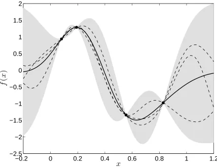
Figure 1 represents a posterior predictive distribution for a data vectorYwithN = 4. Data points are repre-sented as dots in the figure. The solid line represents the mean function predicted,f∗(x∗), while the shaded region

corresponds to two standard deviations away from the mean. This shaded region is specified using the predicted covariance function,k∗(x∗,x∗). Notice how the uncertainty in the prediction increases as we move away from the

data points.

Equations forf∗(x∗)andk∗(x∗,x∗)are obtained under the assumption of a Gaussian likelihood, common in

regression setups. For non-Gaussian likelihoods, for example in classification problems, closed form solutions are not longer possible. In this case, one can resort to different approximations, including the Laplace approximation and variational methods [82].

2.3

A Connection Between Bayesian and Regularization Point of Views

Connections between regularization theory and Gaussian process prediction or Bayesian models for prediction have been pointed out elsewhere [78, 105, 82]. Here we just give a very brief sketch of the argument. We restrict ourselves to finite dimensional RKHS. Under this assumption one can show that every RKHS can be described in terms of a feature map [100], that is a mapΦ :X →Rp

, such that

k(x,x′) =

p X

j=1

−0.2

0

0.2

0.4

0.6

0.8

1

1.2

−2.5

−2

−1.5

−1

−0.5

0

0.5

1

1.5

2

x

f

(

x

)

Figure 1: Example of a predictive posterior distribution inferred withN = 4. The solid line corresponds to the predictive mean, the shaded region corresponds to two standard deviations of the prediction. Dots are values of the output functionY. We have also included some samples from the posterior distribution, shown as dashed lines.

In fact in this case one can show that functions in the RKHS with kernelkcan be written as

fw(x) = p X

j=1 wjΦj₍

x) =hw,Φ(x)i, and kfwkk=kwk.

Then we can build a Gaussian process by assuming the coefficientw=w1, . . . , wp

to be distributed according to a multivariate Gaussian distribution. Roughly speaking, in this case the assumptionf∗∼ GP(0, k)becomes

w∼ N(0,Ip)∝e−k

wk2 .

As we noted before if we assume a Gaussian likelihood we have

P(Y|X, f) =N(f(X), σ2ID)∝e−

1

σ2kfw(X)−Yk2n_,

wherefw(X) = (hw,Φ(x₁)i, . . . ,hw,Φ(xn)i)andkfw(X)−Yk2n= Pn

i=1(hw,Φ(xi)i −yi)2. Then the posterior distribution is proportional to

e−(σ12kfw(X)−Yk2_n+kwk2) ,

We note that in regularization the squared error is often replaced by a more general error termN1 PN

i=1ℓ(f(xi), yi). In a regularization perspective, theloss functionℓ:R×R→R+measure the error we incur when predictingf(x)

in place ofy. The choice of the loss function isproblem dependent. Often used examples are the square loss, the logistic loss or the hinge loss used in support vector machines (see [86]).

The choice of a loss function in a regularization setting can be contrasted to the choice of the likelihood in a Bayesian setting. In this context, the likelihood function models how the observations deviate from the assumed

truemodel in the generative process. The notion of a loss function is philosophically different. It represents the cost we pay for making errors. In Bayesian modeling decision making is separated from inference. In the inference stage the posterior distributions are computed evaluating the uncertainty in the model. The loss function appears only at the second stage of the analysis, known as the decisionstage, and weighs how incorrect decisions are penalized given the current uncertainty. However, whilst the two notions are philosophically very different, we can see that, due to the formulation of the frameworks, the loss function and the log likelihood provide the same role mathematically.

The discussion in the previous sections shows that the notion of a kernel plays a crucial role in statistical modeling both in the Bayesian perspective (as the covariance function of a GP) and the regularization perspective (as a reproducing kernel). Indeed, for scalar valued problems there is a rich literature on the design of kernels (see for example [86, 90, 82] and references therein). In the next sections we show how the concept of a kernel can be used in multi-output learning problems. Before doing that, we describe how the concepts of RKHSs and GPs translate to the setting of vector valued learning.

3

Learning Multiple Outputs with Kernels Methods

In this chapter we discuss the basic setting for learning vector valued functions and related problems (multiclass, multilabel) and then describe how the concept of kernels (reproducing kernels and covariance function for GP) translate to this setting.

3.1

Multi-output Learning

The problem we are interested in is that of learning an unknown functional relationshipfbetween an input space

X, for exampleX =Rp, and an output spaceRD. In the following we will see that the problem can be tackled either assuming thatfbelongs to reproducing kernel Hilbert space of vector valued functions or assuming thatf

is drawn from a vector valued Gaussian process. Before doing this we describe several related settings all falling under the framework of multi-output learning.

The natural extension of the traditional (scalar) supervised learning problem is the one we discussed in the introduction, when the data are pairsS= (X,Y) = (x1, y1), . . . ,(xN, yN). For example this is the typical setting for problems such as motion/velocity fields estimation. A special case is that of multi-category classification problem or multi-label problems, where if we haveD classes each input point can be associated to a (binary) coding vector where, for example1stands for presence (0for absence) of a class instance.The simplest example is the so calledone vs allapproach to multiclass classification which, if we have{1, . . . , D}classes, amounts to the codingi→ei, where(ei)is the canonical basis ofRD.

A more general situation is that where different outputs might have different training set cardinalities, different input points or in the extreme case even different input spaces. More formally, in this case we have a training set

Sd= (Xd,Yd) = (xd,1, yd,1), . . . ,(xd,Nd, yd,Nd)for each componentfd, withd= 1, . . . , D, where the number of

data associated with each output,(Nd)might be different and the input for a component might belong to different input space(Xd).

The terminology used in machine learning often does not distinguish the different settings above and the term multitask learning is often used. In this paper we use the term multi-output learning or vector valued learning to define the general class of problems and use the term multi-task for the case where each component has different inputs. Indeed in this very general situation each component can be thought of as a distinct task possibly related to other tasks (components). In the geostatistics literature, if each output has the same set of inputs the model is calledisotopicandheterotopicif each output to be associated with a different set of inputs [104]. Heterotopic data is further classified intoentirely heterotopic data, where the variables have no sample locations in common, andpartially heterotopic data, where the variables share some sample locations. In machine learning, the partially heterotopic case is sometimes referred to asasymmetric multitask learning[112, 21].

we restrict the presentation to the isotopic setting, though the models can usually readily be extended to the more general setting. We will use the notationXto indicate the collection of all the training input points,{Xj}Nj=1, and Sto denote the collection of all the training data. Also we will use the notationf(X)to indicate a vector valued function evaluated at different training points. This notation has slightly different meaning depending on the way the input points are sampled. If the input to all the components are the same thenX =x1, . . . ,xN andf(X) =

f1(x1), . . . , fD(xN). If the input for the different components are different thenX ={Xd}Dd=1 = X1, . . . ,XD,

whereXd={xd,n}Nn=1andf(X) = (f1(x1,1), . . . , f1(x1,N)), . . . ,(fD(xD,1), . . . , fD(xD,N)).

3.2

Reproducing Kernel for Vector Valued Function

The definition of RKHS for vector valued functions parallels the one in the scalar, with the main difference that the reproducing kernel is nowmatrixvalued, see for example [65, 19] . A reproducing kernel is a symmetric function

K:X × X →RD×D, such that for anyx,x′K(x,x′)is a positive semi-definitematrix. A vector valued RKHS is a Hilbert spaceHof functionsf :X →RD

, such that for veryc∈RD

, andx∈ X,K(x,x′)c, as a function ofx′

belongs toHand moreoverKhas the reproducing property

hf,K(·,x)ciK=f(x)⊤c,

whereh·,·iKis the inner product inH.

Again, the choice of the kernel corresponds to the choice of the representation (parameterization) for the func-tion of interest. In fact any funcfunc-tion in the RKHS is in the closure of the set of linear combinafunc-tions

f(x) =

p X

i=1

K(xi,x)cj, cj∈RD,

where we note that in the above equation each termK(xi,x)is a matrix acting on a vectorcj. The norm in the RKHS typically provides a measure of the complexity of a function and this will be the subject of the next sections. Note that the definition of vector valued RKHS can be described in a component-wise fashion in the following sense. The kernelKcan be described by a scalar kernelRacting jointly on input examples and task indices, that is

(K(x,x′))d,d′ =R((x, d),(x′, d′)), (3)

whereR is a scalar reproducing kernel on the spaceX × {1, . . . , D}. This latter point of view is useful while dealing with multitask learning, see [28] for a discussion.

Provided with the above concepts we can follow a regularization approach to define an estimator by minimiz-ing the regularized empirical error (2), which in this case can be written as

D X

j=1

1

N

N X

i=1

(fj(xi)−yj,i)2+λkfk2K, (4)

wheref= (f1, . . . , fD). Once again the solution is given by the representer theorem [65]

f(x) =

N X

i=1

K(xi,x)ci,

and the coefficient satisfies the linear system

c= (K(X,X) +λNI)−1y, (5) wherec,yare N Dvectors obtained concatenating the coefficients and the output vectors, andK(X,X)is an

N D×N Dwith entries (K(xi,xj))d,d′, fori, j = 1, . . . , N andd, d′ = 1, . . . , D(see for example [65]). More

explicitly

K(X,X) =

    

(K(X1,X1))1,1 · · · (K(X1,XD))1,D

(K(X2,X1))2,1 · · · (K(X2,XD))2,D ..

. · · · ...

(K(XD,X1))D,1 · · · (K(XD,XD))D,D    

where each block(K(Xi,Xj))i,jis anNbyNmatrix (here we make the simplifying assumption that each output has same number of training data). Note that given a new pointx∗the corresponding prediction is given by

f(x∗) =K⊤x_∗c,

whereKx_∗ ∈RD×N Dhas entries(K(x∗,xj))d,d′forj= 1, . . . , Nandd, d′= 1, . . . , D.

3.3

Gaussian Processes for Vector Valued Functions

Gaussian process methods for modeling vector-valued functions follow the same approach as in the single output case. Recall that a Gaussian process is defined as a collection of random variables, such that any finite number of them follows a joint Gaussian distribution. In the single output case, the random variables are associated to a single processfevaluated at different values ofxwhile in the multiple output case, the random variables are associated to different processes{fd}Dd=1, evaluated at different values ofx[24, 37, 102].

The vector-valued functionfis assumed to follow a Gaussian process

f ∼ GP(m,K), (7)

wherem ∈ RD is a vector which components are the mean functions{md(x)}Dd=1 of each output andKis a

positivematrixvalued function as in section 3.2. The entries(K(x,x′))d,d′ in the matrixK(x,x′)correspond to

the covariances between the outputsfd(x)andfd′(x′)and express the degree of correlation or similarity between

them.

For a set of inputsX, the prior distribution over the vectorf(X)is given by

f(X)∼ N(m(X),K(X,X)),

wherem(X)is a vector that concatenates the mean vectors associated to the outputs and the covariance matrix

K(X,X)is the block partitioned matrix in (6). Without loss of generality, we assume the mean vector to be zero. In a regression context, the likelihood function for the outputs is often taken to be Gaussian distribution, so that

p(y|f,x,Σ) =N(f(x),Σ),

whereΣ∈RD×D

is a diagonal matrix with elements3_{σ2

d}Dd=1.

For a Gaussian likelihood, the predictive distribution and the marginal likelihood can be derived analytically. The predictive distribution for a new vectorx∗is [82]

p(f(x∗)|S,f,x∗,φ) =N(f∗(x∗),K∗(x∗,x∗)), (8)

with

f∗(x∗) =K⊤x_∗(K(X,X) +Σ)−1y,

K∗(x∗,x∗) =K(x∗,x∗)−Kx_∗(K(X,X) +Σ)−1K⊤x_∗,

whereΣ = Σ⊗IN, Kx_∗ ∈ RD×N D has entries(K(x∗,xj))d,d′ forj = 1, . . . , N andd, d′ = 1, . . . , D, andφ

denotes a possible set of hyperparameters of the covariance functionK(x,x′)used to computeK(X,X)and the variances of the noise for each output{σ2

d}Dd=1. Again we note that if we are interested into the distribution of

the noisy predictions it is easy to see that we simply have to addPΣto the expression of the prediction variance. The above expression for the mean prediction coincides again with the prediction of the estimator derived in the regularization framework.

In the following chapters we describe several possible choices of kernels (covariance function) for multi-output problems. We start in the next chapter with kernel functions that clearly separate the contributions of input and output. We will see later alternative ways to construct kernel functions that interleave both contributions in a non trivial way.

3_{This relation derives fromy}

d(x) =fd(x) +ǫd(x), for eachd, where{ǫd(x)}Dd=1are independent white Gaussian noise processes with

4

Separable Kernels and Sum of Separable Kernels

In this chapter we review a special class of multi-output kernel functions that can be formulated as a sum of products between a kernel function for the input space alone, and a kernel function that encodes the interactions among the outputs. We refer to this type of multi-output kernel functions asseparable kernelsandsum of separable kernels(SoS kernels).

We consider a class of kernels of the form

(K(x,x′))d,d′ =k(x,x′)kT(d, d′), wherek, kTare scalar kernels onX × X and{1, . . . , D} × {1, . . . , D}.

Equivalently one can consider the matrix expression

K(x,x′) =k(x,x′)B, (9) whereBis aD×D symmetric and positive semi-definite matrix. We call this class of kernels separable since, comparing to (3), we see that the contribution of input and output is decoupled.

In the same spirit a more general class of kernels is given by

K(x,x′) =

Q X

q=1

kq(x,x′)Bq.

For this class of kernels, the kernel matrix associated to a data setXhas a simpler form and can be written as

K(X,X) =

Q X

q=1

Bq⊗kq(X,X), (10)

where⊗represents the Kronecker product between matrices. We call this class of kernels sum of separable kernels (SoS kernels).

The simplest example of separable kernel is given by settingkT(d, d′) = δd,d′, whereδd,d′ is the Kronecker

delta. In this caseB = IN, that is all the outputs are treated as being unrelated. In this case the kernel matrix

K(X,X), associated to some set of dataX, becomes block diagonal. Since the off diagonal terms encode output relatedness. We can see that the matrixBencodes dependencies among the outputs.

The key question is how to choose the scalar kernels{kq}Qq=1and especially how to design, or learn, the

matri-ces{Bq}Qq=1. This is the subject we discuss in the next few sections. We will see that one can approach the problem

from a regularization point of view, where kernels will be defined by the choice of suitable regularizers, or, from a Bayesian point of view, constructing covariance functions from explicit generative models for the different output components. As it turns out these two points of view are equivalent and allow for two different interpretations of the same class of models.

4.1

Kernels and Regularizers

In this section we largely follow the results in [64, 65, 27] and [7]. A possible way to design multi-output kernels of the form (9) is given by the following result. IfKis given by (9) then is possible to prove that the norm of a function in the corresponding RKHS can be written as

kfk2

K=

D X

d,d′₌₁

B†_d,d′hfd, fd′i

k, (11)

whereB†is the pseudoinverse ofBandf= (f1, . . . , fD). The above expression gives another way to see why the matrixBencodes the relation among the components. In fact, we can interpret the right hand side in the above expression as a regularizer inducing specific coupling among different taskshft, ft′i_kwith different weights given

byB†_d,d′. This result says that any such regularizer induces a kernel of the form (9). We illustrate the above idea

Mixed Effect Regularizer Consider the regularizer given by

R(f) =Aω Cω D X

ℓ=1

kfℓk2k+ωD D X

ℓ=1 kfℓ−

1

D

D X

q=1 fqk2k

!

(12)

whereAω = _2(1−ω)(11_−ω+ωD) andCω = (2−2ω+ωD).The above regularizer is composed of two terms: the first is a standard regularization term on the norm of each component of the estimator; the second forces eachfℓ to be close to the mean estimator across the components,f = _D1 PDq=1fq. The corresponding kernel imposes a

common similarity structure between all the output components and the strength of the similarity is controlled by a parameterω,

Kω(x,x′) =k(x,x′)(ω1+ (1−ω)ID) (13) where 1is theD×D matrix whose entries are all equal to1, andk is a scalar kernel on the input spaceX. Settingω = 0corresponds to treating all components independently and the possible similarity among them is not exploited. Conversely,ω= 1is equivalent to assuming that all components are identical and are explained by the same function. By tuning the parameterωthe above kernel interpolates between this two opposites cases. We note that from a Bayesian perspectiveBis a correlation matrix with all the off-diagonals equal toω, which means that the output of the Gaussian process are exchangeable.

Cluster Based Regularizer. Another example of regularizer, proposed in [28], is based on the idea of grouping the components intorclusters and enforcing the components in each cluster to be similar. Following [47], let us define the matrixEas theD×rmatrix, whereris the number of clusters, such thatEℓ,c = 1if the component

lbelongs to clustercand0otherwise. Then we can compute theD×DmatrixM = E(E⊤E)−1E⊤such that

Mℓ,q = _m1_c if componentslandq belong to the same clusterc, andmc is its cardinality,Mℓ,q = 0otherwise. Furthermore letI(c)be the index set of the components that belong to clusterc. Then we can consider the following regularizer that forces components belonging to the same cluster to be close to each other:

R(f) =ǫ1

r X

c=1

X

ℓ∈I(c)

kfℓ−fck

2

k+ǫ2

r X

c=1 mckfck

2

k, (14)

wheref_cis the mean of the components in clustercandǫ1, ǫ2are parameters balancing the two terms.

Straight-forward calculations show that the previous regularizer can be rewritten asR(f) =P_ℓ,qGℓ,qhfℓ, fqi_k, where

Gℓ,q=ǫ1δlq+ (ǫ2−ǫ1)Mℓ,q. (15) Therefore the corresponding matrix valued kernel isK(x,x′) =k(x,x′)G†.

Graph Regularizer. Following [64, 91], we can define a regularizer that, in addition to a standard regulariza-tion on the single components, forces stronger or weaker similarity between them through a givenD×Dpositive weight matrixM,

R(f) =1 2

D X

ℓ,q=1

kfℓ−fqk2kMℓq+ D X

ℓ=1

kfℓk2kMℓ,ℓ. (16)

The regularizerJ(f)can be rewritten as: D

X

ℓ,q=1

kfℓk2kMℓ,q− hfℓ, fqikMℓ,q

+

D X

ℓ=1

kfℓk2kMℓ,ℓ =

D X

ℓ=1 kfℓk2k

D X

q=1

(1 +δℓ,q)Mℓ,q− D X

ℓ,q=1

hfℓ, fqi_kMℓ,q =

D X

ℓ,q=1

hfℓ, fqikLℓ,q (17)

whereL = D−M, withDℓ,q = δℓ,qPDh=1Mℓ,h+Mℓ,q

. Therefore the resulting kernel will beK(x,x′) =

k(x,x′)L†, withk(x,x′)a scalar kernel to be chosen according to the problem at hand.

4.2

Coregionalization Models

The use of probabilistic models and Gaussian processes for multi-output learning was pioneered and largely de-veloped in the context of geostatistics, where prediction over vector-valued output data is known ascokriging. Geostatistical approaches to multivariate modelling are mostly formulated around the “linear model of coregion-alization” (LMC) [49, 37], that can be considered as a generative approach for developing valid covariance func-tions. Covariance functions obtained under the LMC assumption follow the form of a sum of separable kernels. We will start considering this model and then discuss how several models recently proposed in the machine learn-ing literature are special cases of the LMC.

4.2.1 The Linear Model of Coregionalization

In the linear model of coregionalization, the outputs are expressed as linear combinations of independent random functions. This is done in a way that ensures that the resulting covariance function (expressed jointly over all the outputs and the inputs) is a valid positive semidefinite function. Consider a set ofDoutputs{fd(x)}Dd=1with x∈Rp

. In the LMC, each componentfdis expressed as [49]

fd(x) = Q X

q=1

ad,quq(x),

where the latent functionsuq(x), have mean zero and covariancecov[uq(x), uq′(x′)] =k_q(x,x′)ifq=q′, anda_d,q

are scalar coefficients. The processes{uq(x)}qQ=1are independent forq 6=q′. The independence assumption can

be relaxed and such relaxation is presented as an extension in section 4.3. Some of the basic processesuq(x)and

uq′(x′)can have the same covariancekq(x,x′), while remaining independent.

A similar expression for{fd(x)}dD=1can be written grouping the functionsuq(x)which share the same covari-ance [49, 37]

fd(x) = Q X q=1 Rq X i=1 aid,qu

i

q(x), (18)

where the functions ui

q(x), with q = 1, . . . , Q andi = 1, . . . , Rq, have mean equal to zero and covariance

cov[ui q(x), ui

′

q′(x′)] =kq(x,x′)ifi =i′andq =q′. Expression (18) means that there areQgroups of functions

ui

q(x)and that the functionsu i

q(x)within each group share the same covariance, but are independent. The cross covariance between any two functionsfd(x)andfd′(x)is given in terms of the covariance functions forui_q(x)

cov[fd(x), fd′(x′)] =

Q X

q=1

Q X

q′₌₁

Rq

X

i=1

Rq

X

i′₌₁

aid,qa i′

d′_,q′cov[ui_q(x), ui ′

q′(x′)].

The covariancecov[fd(x), fd′(x′)]is given by(K(x,x′))_d,d′. Due to the independence of the functionsui_q(x), the

above expression reduces to

(K(x,x′))d,d′ =

Q X q=1 Rq X i=1 aid,qa

i

d′_,qkq(x,x′) = Q X

q=1

bq_d,d′kq(x,x′), (19)

withbq d,d′ =

PRq

i=1a

i d,qa

i

d′,q. The kernelK(x,x′)can now be expressed as

K(x,x′) =

Q X

q=1

Bqkq(x,x′), (20)

where eachBq ∈RD×Dis known as acoregionalization matrix. The elements of eachBqare the coefficientsbq_d,d′

appearing in equation (19). The rank for each matrixBqis determined by the number of latent functions that share the same covariance functionkq(x,x′), that is, by the coefficientRq.

Equation (18) can be interpreted as a nested structure [104] in which the outputsfd(x)are first expressed as a linear combination of spatially uncorrelated processesfd(x) =PQq=1f

q

d(x),withE[f q

d(x)] = 0andcov[f q d(x), f

q′ d′(x′)] =

bq

of uncorrelated functions weighted by the coefficientsai d,q,fq

d(x) = PRq

i=1a

i d,qu

i

q(x)where again, the covariance function forui

q(x)iskq(x,x′).

Therefore, starting from a generative model for the outputs, the linear model of coregionalization leads to a sum of separable kernels that represents the covariance function as the sum of the products of two covariance functions, one that models the dependence between the outputs, independently of the input vectorx(the coregionalization matrixBq), and one that models the input dependence, independently of the particular set of functions{fd(x)} (the covariance functionkq(x,x′)). The covariance matrix forf(X)is given by (10).

4.2.2 Intrinsic Coregionalization Model

A simplified version of the LMC, known as the intrinsic coregionalization model (ICM) (see [37]), assumes that the elementsbq

d,d′of the coregionalization matrixBqcan be written asb_d,dq ′ = υd,d′bq, for some suitable coefficients

υd,d′. With this form forbq

d,d′, we have

cov[fd(x), fd′(x′)] =

Q X

q=1

υd,d′bqkq(x,x′),=υd,d′

Q X

q=1

bqkq(x,x′)

=υd,d′k(x,x′),

wherek(x,x′) =PQq=1bqkq(x,x′). The above expression can be seen as a particular case of the kernel function ob-tained from the linear model of coregionalization, withQ= 1. In this case, the coefficientsυd,d′=PR_i=11 ai_d,1ai_d′_,1=

b1

d,d′, and the kernel matrix for multiple outputs becomesK(x,x′) =k(x,x′)Bas in (9).

The kernel matrix corresponding to a datasetXtakes the form

K(X,X) =B⊗k(X,X). (21) One can see that the intrinsic coregionalization model corresponds to the special separable kernel often used in the context of regularization. Notice that the value ofR1for the coefficientsυd,d′ =PR_i=11 a_d,i₁ai_d′,1=b1d,d′, determines

the rank of the matrixB.

As pointed out by [37], the ICM is much more restrictive than the LMC since it assumes that each basic covari-ancekq(x,x′)contributes equally to the construction of the autocovariances and cross covariances for the outputs. However, the computations required for the corresponding inference are greatly simplified, essentially because of the properties of the Kronecker product. This latter point is discussed in detail in Section 6.

It can be shown that if the outputs are considered to be noise-free, prediction using the intrinsic coregional-ization model under an isotopic data case is equivalent to independent prediction over each output [41]. This circumstance is also known as autokrigeability [104].

4.2.3 Comparison Between ICM and LMC

We have seen before that the intrinsic coregionalization model is a particular case of the linear model of core-gionalization forQ= 1(withRq 6= 1) in equation 19. Here we contrast these two models. Note that a different particular case of the linear model of coregionalization is assumingRq = 1(withQ6= 1). This model, known in the machine learning literature as the semiparametric latent factor model (SLFM) [96], will be introduced in the next subsection.

To compare the two models we have sampled from a multi-output Gaussian process with two outputs (D= 2), a one-dimensional input space (x∈R) and a LMC with different values forRqandQ. As basic kernelskq(x,x′) we have used the exponentiated quadratic (EQ) kernel given as [82],

kq(x,x′) = exp

−kx−x

′_k2 ℓ2

q

,

wherek·krepresents the Euclidian norm andℓqis known as the characteristic length-scale. The exponentiated quadratic is variously referred to as the Gaussian, the radial basis function or the squared exponential kernel.

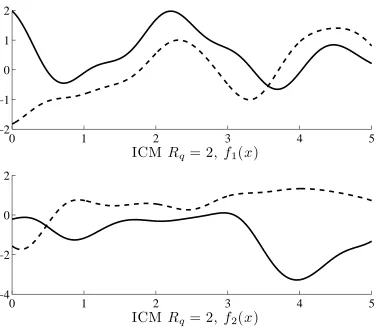
Figure 2 shows samples from the intrinsic coregionalization model forRq = 1, meaning a coregionalization matrixB1of rank one. Samples share the same length-scale and have similar form. They have different variances,

though. Each sample may be considered as a scaled version of the latent function, as it can be seen from equation 18 withQ= 1andRq= 1,

0

1

2

3

4

5

−1

0

1

2

ICM

R

q

= 1,

f

1

(

x

)

0

1

2

3

4

5

−5

0

5

10

ICM

R

q

= 1,

f

2

(

x

)

Figure 2: Two samples from the intrinsic coregionalization model with rank one, this is Rq = 1. Solid lines represent one of the samples, and dashed lines represent the other sample. Samples are identical except for scale.

where we have usedxinstead ofxfor the one-dimensional input space.

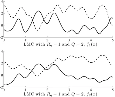
Figure 3 shows samples from an ICM of rank two. From equation 18, we have forQ= 1andRq= 2,

f1(x) =a11,1u11(x) +a21,1u21(x), f2(x) =a12,1u11(x) +a22,1u21(x),

whereu11(x)andu21(x)are sampled from the same Gaussian process. Outputs are weighted sums of two different

latent functions that share the same covariance. In contrast to the ICM of rank one, we see from figure 3 that both outputs have different forms, although they share the same length-scale.

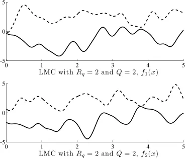
Figure 4 displays outputs sampled from a LMC withRq = 1and two latent functions (Q= 2) with different scales. Notice that both samples are combinations of two terms, a long scale term and a short length-scale term. According to equation 18, outputs are given as

f1(x) =a11,1u11(x) +a11,2u12(x), f2(x) =a12,1u11(x) +a12,2u12(x),

whereu1

1(x)andu12(x)are samples from two Gaussian processes with different covariance functions. In a similar

way to the ICM of rank one (see figure 2), samples from both outputs have the same form, this is, they are aligned. We have the additional case for a LMC withRq = 2andQ = 2in figure 5. According to equation 18, the outputs are give as

0

1

2

3

4

5

−2

−1

0

1

2

ICM

R

q

= 2,

f

1

(

x

)

0

1

2

3

4

5

−4

−2

0

2

ICM

R

q

= 2,

f

2

(

x

)

Figure 3: Two samples from the intrinsic coregionalization model with rank two,Rq = 2. Solid lines and dashed lines represent different samples. Although samples from different outputs have the same length-scale, they look different and are not simply scaled versions of one another.

where the pair of latent functionsu1

1(x)andu21(x)share their covariance function and the pair of latent functions u12(x)andu22(x)also share their covariance function. As in the case of the LMC withRq = 1andQ= 2in figure 4, the outputs are combinations of a term with a long length-scale and a term with a short length-scale. A key difference however, is that, forRq= 2andQ= 2, samples from different outputs have different shapes.4

4.2.4 Linear Model of Coregionalization in Machine Learning and Statistics

The linear model of coregionalization has already been used in machine learning in the context of Gaussian pro-cesses for multivariate regression and in statistics for computer emulation of expensive multivariate computer codes.

As we have seen before, the linear model of coregionalization imposes the correlation of the outputs explicitly through the set of coregionalization matrices. A simple idea used in the early papers of multi-output GPs for machine learning was based on the intrinsic coregionalization model and assumedB=ID. In other words, the outputs were considered to be conditionally independent given the parametersφ. Correlation between the outputs was assumed to exist implicitly by imposing the same set of hyperparametersφfor all outputs and estimating those parameters, or the kernel matrixk(X,X)directly, using data from all the outputs [66, 55, 113].

4_{Notice that samples from each output are not synchronized, meaning that the maximums and minimus do not always occur at the same}

0

1

2

3

4

5

−2

0

2

4

LMC with

R

q

= 1 and

Q

= 2,

f

1

(

x

)

0

1

2

3

4

5

−2

0

2

4

LMC with

R

q

= 1 and

Q

= 2,

f

2

(

x

)

Figure 4: Two samples from a linear model of coregionalization withRq = 1andQ= 2. The solid lines represent one of the samples. The dashed lines represent the other sample. Samples are the weigthed sums of latent functions with different length-scales.

In this section, we review more recent approaches for multiple output modeling that are different versions of the linear model of coregionalization.

Semiparametric latent factor model. The semiparametric latent factor model (SLFM) proposed by [96] turns out to be a simplified version of the LMC. In fact it corresponds to settingRq = 1in (18) so that we can rewrite equation (10) as

K(X,X) =

Q X

q=1

aqa⊤q ⊗kq(X,X),

where aq ∈ RD×1 with elements{ad,q}Dd=1 andqfixed. With some algebraic manipulations, that exploit the

properties of the Kronecker product, we can write

K(X,X) =

Q X

q=1

(aq⊗IN)kq(X,X)(a⊤q ⊗IN) = (Ae⊗IN)Ke(Ae⊤⊗IN),

whereAe∈RD×Q

is a matrix with columnsaqandKe ∈RQN×QN is a block diagonal matrix with blocks given by

0

1

2

3

4

5

−5

0

5

LMC with

R

= 2 and

Q

= 2,

f

(

x

)

0

1

2

3

4

5

−5

0

5

LMC with

R

= 2 and

Q

= 2,

f

(

x

)

Figure 5: Two samples from a linear model of coregionalization withRq = 2andQ= 2. The solid lines represent one of the samples. The dashed lines represent the other sample. Samples are the weigthed sums of four latent functions, two of them share a covariance with a long length-scale and the other two share a covariance with a shorter length-scale.

The functionsuq(x) are considered to be latent factors and the semiparametric name comes from the fact that it is combining a nonparametric model, that is a Gaussian process, with a parametric linear mixing of the functionsuq(x). The kernelskq, for each basic process is assumed to be exponentiated quadratic with a different characteristic length-scale for each input dimension. The informative vector machine (IVM) [57] is employed to speed up computations.

Gaussian processes for Multi-task, Multi-output and Multi-class The intrinsic coregionalization model is considered by [12] in the context of multitask learning. The authors use a probabilistic principal component analysis (PPCA) model to represent the matrixB. The spectral factorization in the PPCA model is replaced by an incomplete Cholesky decomposition to keep numerical stability. The authors also refer to the autokrigeability effect as the cancellation of inter-task transfer [12], and discuss the similarities between the multi-task GP and the ICM, and its relationship to the SLFM and the LMC.

The intrinsic coregionalization model has also been used by [72]. Here the matrixB is assumed to have a spherical parametrization,B= diag(e)S⊤Sdiag(e), whereegives a description for the scale length of each output variable andSis an upper triangular matrix whosei-th column is associated with particular spherical coordinates of points inRi

(for details see sec. 3.4 [71]). The scalar kernelkis represented through a Mat´ern kernel, where different parameterizations allow the expression of periodic and non-periodic terms. Sparsification for this model is obtained using an IVM style approach.

outputs are conditionally independent given the hyperparametersφ[66, 110, 55, 89, 113, 82]. Therefore, the kernel matrixK(X,X)takes a block-diagonal form, with blocks given by(K(Xd,Xd))d,d. Correlation between the out-puts is assumed to exist implicitly by imposing the same set of hyperparametersφfor all outputs and estimating those parameters, or directly the kernel matrices(K(Xd,Xd))d,d, using data from all the outputs [66, 55, 113, 82]. Alternatively, it is also possible to have parametersφdassociated to each output [110, 89].

Only recently, the intrinsic coregionalization model has been used in the multiclass scenario. In [93], the authors use the intrinsic coregionalization model for classification, by introducing a probit noise model as the likelihood. Since the posterior distribution is no longer analytically tractable, the authors use Gibbs sampling, Expectation-Propagation (EP) and variational Bayes5_{to approximate the distribution.}

Computer emulation. A computer emulator is a statistical model used as a surrogate for a computationally expensive deterministic model or computer code, also known as a simulator. Gaussian processes have become the preferred statistical model among computer emulation practitioners (for a review see [70]). Different Gaussian process emulators have been recently proposed to deal with several outputs [42, 23, 83, 63, 9, 79].

In [42], the linear model of coregionalization is used to model images representing the evolution of the implo-sion of steel cylinders after using TNT and obtained employing the so called Neddemeyer simulation model (see [42] for further details). The input variablexrepresents parameters of the simulation model, while the output is an image of the radius of the inner shell of the cylinder over a fixed grid of times and angles. In the version of the LMC that the authors employed,Rq = 1and theQvectorsaqwere obtained as the eigenvectors of a PCA decomposition of the set of training images.

In [23], the intrinsic coregionalization model is employed for emulating the response of a vegetation model called the Sheffield Dynamic Global Vegetation Model (SDGVM) [111]. Authors refer to the ICM as the Multiple-Output (MO) emulator. The inputs to the model are ten (p= 10) variables related to broad soil, vegetation and climate data, while the outputs are time series of the net biome productivity (NBP) index measured at a particular site in a forest area of Harwood, UK. The NBP index accounts for the residual amount of carbon at a vegetation site after some natural processes have taken place. In the paper, the authors assume that the outputs correspond to the different sampling time points, so thatD=T, beingT the number of time points, while each observation corresponds to specific values of the ten input variables. Values of the input variables are chosen according to a maxi-min Latin hypercube design.

Rougier [83] introduces an emulator for multiple-outputs that assumes that the set of output variables can be seen as a single variable while augmenting the input space with an additional index over the outputs. In other words, it considers the output variable as an input variable. [23], refers to the model in [83] as the Time Input (TI) emulator and discussed how the TI model turns out to be a particular case of the MO model that assumes a particular exponentiated quadratic kernel (see chapter 4 [82]) for the entries in the coregionalization matrixB.

McFarlandet al. [63] consider a multiple-output problem as a single output one. The setup is similar to the one used in [23], where the number of outputs are associated to different time points, this is,D=T. The outputs correspond to the time evolutions of the temperature of certain location of a container with decomposing foam, as function of five differentcalibrationvariables (input variables in this context,p= 5). The authors use the time index as an input (akin to [83]) and apply a greedy-like algorithm to select the training points for the Gaussian process. Greedy approximations like this one have also been used in the machine learning literature (for details, see [82], page 174).

Similar to [83] and [63], Bayarriet al.[9] use the time index as an input for a computer emulator that evaluates the accuracy of CRASH, a computer model that simulates the effect of a collision of a vehicle with different types of barriers.

Quianet al. [79] propose a computer emulator based on Gaussian processes that supports quantitative and qualitative inputs. The covariance function in this computer emulator is related to the ICM in the case of one qualitative factor: the qualitative factor is considered to be the index of the output, and the covariance function takes again the formk(x,x′)kT(d, d′). In the case of more than one qualitative input, the computer emulator could be considered a multiple output GP in which each output index would correspond to a particular combination of the possible values taken by the qualitative factors. In this case, the matrixBin ICM would have a block diagonal form, each block determining the covariance between the values taken by a particular qualitative input.

4.3

Extensions

In this section we describe further developments related to the setting of separable kernels or SoS kernels, both from a regularization and a Bayesian perspective.

4.3.1 Extensions Within the Regularization Framework

When we consider kernels of the formK(x,x′) =k(x,x′)B, a natural question is whether the matrixBcan be learned from data. In a regression setting, one idea is to estimateBin a separate inference step as the covariance matrix of the output vectors in the training set and this is standard in the geostatistics literature [104]. A further question is whether we can learn bothBand an estimator within a unique inference step. This is the question tackled in [48]. The authors consider a variation of the regularizer in (14) and try to learn the cluster matrix as a part of the optimization process. More precisely the authors considered a regularization term of the form

R(f) =ǫ1kfkk+ǫ2

r X

c=1

mckfc−fk

2

k+ǫ3

r X

c=1

X

l∈I(c) kfl

−f_ck2k, (22)

where we recall thatris the number of clusters. The three terms in the functional can be seen as: a global penalty, a term penalizingbetween clustervariance and a term penalizingwithin clustervariance. As in the case of the regularizer in (14), the above regularizer is completely characterized by a cluster matrixM, i.e. R(f) = RM(f)

(note that the corresponding matrixBwill be slightly different from (15)). The idea is then to consider a regularized functional

D X i=1 1 N N X i=1

(fj(xi)−yj,i)2+λRM(f) (23)

to be minimized jointly overfandM(see [48] for details). This problem is typically non tractable from a com-putational point of view, so the authors in [48] propose a relaxation of the problem which can be shown to be convex.

A different approach is taken in [4] and [5]. In this case the idea is that only a a small subset of features is useful to learn all the components/tasks. In the simplest case the authors propose to minimize a functional of the form

D X d=1 ( 1 N N X i=1

(w⊤dU⊤xi−yd,i)2+λw⊤dwd )

.

overw1, . . . ,wD ∈ Rp, U ∈ RD×Dunder the constraint Tr(Ut⊤Ut) ≤ γ. Note that the minimization over the matrix U couples the otherwise disjoint component-wise problems. The authors of [4] discuss how the above model is equivalent to considering a kernel of the form

K(x,x′) =kD(x,x′)ID, kD(x,x′) =x⊤Dx′

whereDis a positive definite matrix and a model which can be described components wise as

fd(x) = p X

i=1

ad,ixj=a⊤dx,

making apparent the connection with the LMC model. In fact, it is possible to show that the above minimization problem is equivalent to minimizing

D X d=1 1 N N X i=1

(a⊤dxi−yd,i)2+λ D X

d=1

a⊤dDad, (24)

overa′1, . . . ,a′D ∈ R p

above framework to the case of more general kernel functions. Note that an approach similar to the one we just described is at the basis of recent work exploiting the concept of sparsity while solving multiple tasks. These latter methods cannot in general be cast in the framework of kernel methods and we refer the interested reader to [69] and references therein.

For the reasoning above the key assumption is that a response variable is either important for all the tasks or not. In practice it is probably often the case that only certain subgroups of tasks share the same variables. This idea is at the basis of the study in [5], where the authors design an algorithm to learn at once the group structure and the best set of variables for each groups of tasks. LetG = (Gt)⊤t=1be a partition of the set of components/tasks,

whereGtdenotes a group of tasks and|Gt| ≤D. Then the author propose to consider a functional of the form

min

G

X

Gt∈G

min

a_d,d∈Gt,Ut

X

d∈Gt

(

1

N

N X

i=1

(a⊤dUt⊤xi−yd,i)2+λw⊤dw⊤d

+γTr(Ut⊤Ut) )

,

whereU1, . . . UT is a sequence ofpbypmatrices. The authors show that while the above minimization problem is not convex, stochastic gradient descent can be used to find local minimizers which seems to perform well in practice.

4.3.2 Extensions from the Gaussian Processes Perspective

A recent extension of the linear model of coregionalization expresses the output covariance function through a linear combination of nonorthogonal latent functions [39]. In particular, the basic processesui

q(x)are assumed to be nonorthogonal, leading to the following covariance function

cov[f(x),f(x′)] =

Q X

q=1

Q X

q′₌₁

Bq,q′k_q,q′(x,x′),

whereBq,q′ arecross-coregionalizationmatrices. Cross-covariancesk_q,q′(x,x′)can be negative (while keeping

pos-itive semidefiniteness forcov[f(x),f(x′)]), allowing negative cross-covariances in the linear model of coregional-ization. The authors argue that, in some real scenarios, a linear combination of several correlated attributes are combined to represent a single model and give examples in mining, hydrology and oil industry [39].

5

Beyond Separable Kernels

Working with separable kernels or SoS kernels is appealing for their simplicity, but can be limiting in several applications. Next we review different types of kernels that go beyond the separable case or SoS case.

5.1

Invariant Kernels

Divergence free and curl free fields. The following two kernels are matrix valued exponentiated quadratic (EQ) kernels [68] and can be used to estimate divergence-free or curl-free vector fields [60] when the input and output space have the same dimension. These kernels induce a similarity between the vector field components that depends on the input points, and therefore cannot be reduced to the formK(x,x′) =k(x,x′)B.

We consider the case of vector fields withD =p, whereX =Rp

. The divergence-free matrix-valued kernel can be defined via a translation invariant matrix-valued EQ kernel

Φ(u) = (∇∇⊤− ∇⊤∇I)φ(u) =Hφ(u)−tr(Hφ(u))ID, whereHis the Hessian operator andφa scalar EQ kernel, so thatK(x,x′) := Φ(x−x′).

The columns of the matrix valued EQ kernel,Φ, are divergence-free. In fact, computing the divergence of a linear combination of its columns,∇⊤_(Φ(u)c)

, withc∈Rp

, it is possible to show that [7]

where the last equality follows applying the product rule of the gradient, the fact that the coefficient vectorcdoes not depend uponuand the equalitya⊤aa⊤=a⊤a⊤a,∀a∈Rp.

Choosing a exponentiated quadratic, we obtain the divergence-free kernel

K(x,x′) = 1

σ2e

−kx−x′k2

2σ2 _Ax

,x′, (25)

where

Ax,x′ = x−x

′

σ

x−x′

σ

⊤

+

(p−1)−kx−x

′_k2 σ2

Ip !

.

The curl-free matrix valued kernels are obtained as

K(x,x′) := Ψ(x−x′) =−∇∇⊤φ(x−x′) =−Hφ(x−x′),

whereφis a scalar RBF. It is easy to show that the columns ofΨare curl-free. Thej-th column ofΨis given by

Ψej, whereejis the standard basis vector with a one in thej-th position. This gives us

Φcfej=−∇∇⊤Φcfej=∇(−∇⊤Φcfej) =∇g ,

whereg=−∂φ/∂xj. The functiongis a scalar function and the curl of the gradient of a scalar function is always zero. Choosing a exponentiated quadratic, we obtain the following curl-free kernel

Γcf(x,x′) =

1

σ2e

−kx−x′k2

2σ2 _ID−

x−x′

σ

x−x′

σ

⊤!

. (26)

It is possible to consider a convex linear combination of these two kernels to obtain a kernel for learning any kind of vector field, while at the same time allowing reconstruction of the divergence-free and curl-free parts separately (see [60]). The interested reader can refer to [68, 59, 32] for further details on matrix-valued RBF and the properties of divergence-free and curl-free kernels.

Transformable kernels. Another example of invariant kernels is discussed in [18] and is given by kernels defined by transformations. For the purpose of our discussion, letY = RD,X0 be a Hausdorff space andTda family of maps (not necessarily linear) fromX toX0ford={1, . . . , D}.

Then, given a continuous scalar kernelk :X0× X0 →R, it is possible to define the following matrix valued

kernel for anyx,x′∈ X

K(x,x′)

d,d′ =k(Tdx, Td ′x′).

A specific instance of the above example is described by [101] in the context of system identification, see also [18] for further details.

5.2

Further Extensions of the LMC

In [34], the authors introduced a nonstationary version of the LMC, in which the coregionalization matrices are allowed to vary as functions of the input variables. In particular,Bqnow depends on the input variablex, this is,

Bq(x,x′). The authors refer to this model as the spatially varying LMC (SVLMC). As a model for the varying core-gionalization matrixBq(x,x′), the authors employ two alternatives. In one of them, they assume thatBq(x,x′) =

(α(x,x′))ψ

Bq, whereα(x)is a covariate of the input variable, andψis a variable that follows a uniform prior. In the other alternative,Bq(x,x′)follows a Wishart spatial process, which is constructed using the definition of a Wishart distribution, as follows. SupposeZ∈RD×P is a random matrix with entrieszd,p ∼ N(0,1), indepen-dently and identically distributed, ford= 1, . . . , Dandp= 1, . . . , P. Define the matrixΥ=ΓZ, withΓ∈RD×D

. The matrixΩ =ΥΥ⊤ = ΓZZ⊤Γ⊤ ∈RD×Dfollows a Wishart distributionW(P,ΓΓ⊤), whereP is known as thenumber of degrees of freedomof the distribution. The spatial Wishart process is constructed assuming thatzd,p depends on the inputx, this is,zd,p(x,x′), withzd,p(x,x′)∼ N(0, ρd(x,x′)), where{ρd(x,x′)}Dd=1are correlation

functions. MatrixΥ(x,x′) = ΓZ(x,x′)andΩ(x,x′) = Υ(x,x′)Υ⊤(x,x′) = ΓZ(x,x′)Z⊤(x,x′)Γ⊤ ∈ RD×D

5.3

Process Convolutions

More general non-separable kernels can also be constructed from a generative point of view. We saw in section 4.2.1 that the linear model of coregionalization involves instantaneous mixing through a linear weighted sum of independent processes to construct correlated processes. By instantaneous mixing we mean that the output functionf(x)evaluated at the input pointxonly depends on the values of the latent functions{uq(x)}Qq=1at the

same inputx. This instantaneous mixing leads to a kernel function for vector-valued functions that has a separable form.

A non-trivial way to mix the latent functions is through convolving a base process with a smoothing kernel.6_If

the base process is a Gaussian process, it turns out that the convolved process is also a Gaussian process. We can therefore exploit convolutions to construct covariance functions [8, 102, 43, 44, 14, 56, 2].

In a similar way to the linear model of coregionalization, we considerQgroups of functions, where a particular groupqhas elementsui

q(z), fori= 1, . . . , Rq. Each member of the group has the same covariancekq(x,x′), but is sampled independently. Any outputfd(x)is described by

fd(x) = Q X q=1 Rq X i=1 Z X Gi

d,q(x−z)u i

q(z)dz+wd(x) = Q X

q=1 fq

d(x) +wd(x),

where

fdq(x) = Rq

X

i=1

Z

X

Gid,q(x−z)u i

q(z)dz, (27)

and{wd(x)}Dd=1are independent Gaussian processes with zero mean and covariancekwd(x,x

′₎

. For the integrals in equation (27) to exist, it is assumed that each kernelGi

d,q(x)is a continuous function with compact support [46] or square-integrable [102, 44]. The kernelGi

d,q(x)is also known as the moving average function [102] or the smoothing kernel [44]. We have included the superscriptqforfq

d(x)in (27) to emphasize the fact that the function depends on the set of latent processes{ui

q(x)} Rq

i=1. The latent functionsu

i

q(z)are Gaussian processes with general covarianceskq(x,x′).

Under the same independence assumptions used in the linear model of coregionalization, the covariance be-tweenfd(x)andfd′(x′)follows

(K(x,x′))d,d′=

Q X

q=1 kf_dq,fq

d′(x,x

′_{) +k}

wd(x,x

′_)δ

d,d′, (28)

where

kf_dq,fq

d′(x,x

′_{) =} Rq X i=1 Z X Gi

d,q(x−z) Z

X

Gi

d′_,q(x′−z′)kq(z,z′)dz′dz. (29)

SpecifyingGi

d,q(x−z)andkq(z,z′)in the equation above, the covariance for the outputsfd(x)can be constructed indirectly. Notice that if the smoothing kernels are taken to be the Dirac delta function in equation (29), such thatGi

d,q(x−z) = a i

d,qδ(x−z),7the double integral is easily solved and the linear model of coregionalization is recovered. In this respect, process convolutions could also be seen as a dynamic version of the linear model of coregionalization in the sense that the latent functions are dynamically transformed with the help of the kernel smoothing functions, as opposed to a static mapping of the latent functions in the LMC case. See section 5.3.1 for a comparison between the process convolution and the LMC.

A recent review of several extensions of this approach for the single output case is presented in [17]. Some of those extensions include the construction of nonstationary covariances [43, 45, 30, 31, 73] and spatiotemporal covariances [109, 107, 108].

The idea of using convolutions for constructing multiple output covariances was originally proposed by [102]. They assumed thatQ= 1,Rq = 1, that the processu(x)was white Gaussian noise and that the input space was

6_{We use kernel to refer to both reproducing kernels and smoothing kernels. Smoothing kernels are functions which are convolved with a}

signal to create a smoothed version of that signal.

7_{We have slightly abused of the delta notation to indicate the Kronecker delta for discrete arguments and the Dirac function for continuous}