Analysis of the use of genetic algorithms for indoor localisation via cloud point matching

This is a repository copy of

Analysis of the use of genetic algorithms for indoor localisation

via cloud point matching

.

White Rose Research Online URL for this paper:

http://eprints.whiterose.ac.uk/131751/

Version: Accepted Version

Proceedings Paper:

Boland, Miguel and Soares Indrusiak, Leandro orcid.org/0000-0002-9938-2920 (Accepted:

2018) Analysis of the use of genetic algorithms for indoor localisation via cloud point

matching. In: Proceedings of the Genetic and Evolutionary Computation Conference. The

Genetic and Evolutionary Computation Conference, 15-19 Jul 2018 . (In Press)

https://doi.org/10.1145/3205455.3205499

[email protected]

https://eprints.whiterose.ac.uk/

Reuse

Items deposited in White Rose Research Online are protected by copyright, with all rights reserved unless

indicated otherwise. They may be downloaded and/or printed for private study, or other acts as permitted by

national copyright laws. The publisher or other rights holders may allow further reproduction and re-use of

the full text version. This is indicated by the licence information on the White Rose Research Online record

for the item.

Takedown

If you consider content in White Rose Research Online to be in breach of UK law, please notify us by

via cloud point matching

Miguel d. Boland

[email protected] University of York

Leandro Soares Indrusiak

University of York

ABSTRACT

A system’s ability to precisely locate itself in a known physical environment is key to its capacity to interact with the environment in an intricate manner. The indoor localisation problem has been approached in a variety of ways, ranging from the identiication of pre-deined features or topologies to the more general cloud-point matching.

Cloud point matching can be achieved using a variety of algo-rithms, each with beneits and drawbacks. Recent improvements have focused on the application of genetic algorithms to solve the initial ’global’ search for a solution, before reining this solution to a precise position through a non-genetic algorithm. This project aims to demonstrate the ineiciency of genetic algorithms applied to the global search problem for the issue of indoor localisation; this is thought to be caused by the solution space’s low dimensionality, so-lution landscape topology and the ineicacy of crossover operators in the algorithm. Based on our assumptions of map topologies, we conclude that signiicant redundancies can be found in some purely genetic heuristics and suggest further development of landscape analysis to allow the use of algorithms appropriate to the scenario’s complexity.

CCS CONCEPTS

·Computer systems organization→Embedded systems; Re-dundancy; Robotics; ·Networks→ Network reliability;

KEYWORDS

Genetic Algorithms, Indoor Localisation, R

ACM Reference Format:

Miguel d. Boland and Leandro Soares Indrusiak. 2018. Analysis of the use of genetic algorithms for indoor localisation via cloud point matching. In GECCO ’18: Genetic and Evolutionary Computation Conference, July 15ś19, 2018, Kyoto, Japan.ACM, New York, NY, USA, 8 pages. https:⁄⁄doi.org⁄10. 1145⁄3205455.3205499

Permission to make digital or hard copies of all or part of this work for personal or classroom use is granted without fee provided that copies are not made or distributed for proit or commercial advantage and that copies bear this notice and the full citation on the irst page. Copyrights for components of this work owned by others than ACM must be honored. Abstracting with credit is permitted. To copy otherwise, or republish, to post on servers or to redistribute to lists, requires prior speciic permission and⁄or a fee. Request permissions from [email protected].

GECCO ’18, July 15ś19, 2018, Kyoto, Japan

© 2018 Association for Computing Machinery. ACM ISBN 978-1-4503-5618-3⁄18⁄07. . . $15.00 https:⁄⁄doi.org⁄10.1145⁄3205455.3205499

1

INTRODUCTION

The problem of line-of-sight indoor localisation was irst resolved through the matching of cloud point data (obtained from a

line-of-sight sensor such as a Li-Dar) to retrieve tuple(x,y,θ)describing

the location and orientation of a robot in a known environment. This was irst achieved by algorithms such as the Iterative Closest Point (ICP) algorithm Besl and McKay [4], and a long line of alterna-tive heuristic algorithms Lu and Milios [23], Diosi and Kleeman [11] [29], Biber and Strasser [5], Donoso-Aguirre et al. [13], Konecny et al. [19] and various improvements on the ICP’s convergence speed [12] [32], dataset optimisation [33] [25] or precision metrics [14].

Performing indoor localisation without a priori knowledge of the robot’s pose increases the diiculty to this problem, as a global search for the position must now be performed, rather than simply a pose reinement. Using test cases from Lenac et al. [20], we

ini-Scan 18 Scan 110

Scan 115 Scan 240

Figure 1: Fitness landscapes for randomly selected scans in dataset.

GECCO ’18, July 15–19, 2018, Kyoto, Japan

generally computationally less eicient". Given the full knowledge of the map and scan data, and the relative ease with which we can construct a itness landscape relating the two, we can see that the general problem deinition contrasts greatly with intended applica-tions of genetic algorithms.

Ωe therefore aim to demonstrate redundancies in the behaviour of genetic algorithms applied to a subset of the indoor localisation problem with knowledge of the environment but no a priori pose. This is achieved by creating improvements to a benchmark ge-netic algorithms to demonstrate the ability of a simple non-gege-netic heuristic algorithm to outperform a genetic algorithm in terms of eiciency, as measured by pose precision and computational time.

2

EXISTING WORK

The use of genetic algorithms to search for data-matching solutions was pioneered by Brunnstrom and Stoddart [7] to ind the corre-spondences between detailed surface models. This was achieved by using a chromosome design based on a transformation, translation and rotation in three dimensions. A simpliied X⁄Y translation and rotation chromosome is used as the basis for all further genetic algorithms for 2D indoor localisation.

Robertson and Fisher [30] later presented a GA alternative to the ICP algorithm to avoid requiring a priori pose knowledge and the tendency to converge to sub-optimal or incorrect solutions. These were solved through the GA’s ability to search for a global maxima, rather than simply reine a pose to the local minima. This is implemented using a 3-tuple matching our problem deinition (x,y,θ), and results in signiicantly better global search results than a single ICP run, thereby demonstrating the potential of genetic algorithms within the ield.

Polar Scan matching (PSM) is a variation of Robertson and Fisher’s initial genetic algorithm which is adapted for the direct use of raw data from a laser range scanner, therefore reducing the computational costs of the operation. Ze-Su et al. [35] believe this

would represent twoO(n)searches: one for the translation

estima-tion, and one for the orientation estimation. This approach is found to be more precise and eicient than ICP in the given examples [35], although given the variation in performance of algorithms in scenes [12] this result may not be generalisable. As demonstrated by Ze-Su et al., the method is applied to identify two complete sets of data, rather than mapping a subset of the data (the area visible around the robot) into the full set of data (the full map); further adaptation may therefore be required for the method to function for general indoor localisation.

Recent improvements in the performance of GAs were suggested by Lenac et al., but involve a trade-of in accuracy with execution time due to the use of a rasterized environment.

The concept of combining the global search of a GA with the accuracy of the ICP algorithm has been introduced in a variety of concepts. Brunnstrom and Stoddart [7] irst proposed the idea of applying a low-accuracy global search using a GA, before rein-ing the most promisrein-ing individual poses usrein-ing an ICP algorithm using the pre-aligned poses. Using a itness function deined by minimising the sum of the distance between pairs of closest points (each pair composed of a point in the scan and a point in the map),

Brunnstrom and Stoddart presents an objective set of results demon-strating the algorithms ability to roughly estimate the 3-tuple pose modiication, but produces no statistical data regarding the success rate or accuracy of the algorithm.

The hybrid approach was independently presented by Martínez et al. [24], resulting in a method which is indistinguishable from a standard GA, but is however quicker to execute as the GA search can be completed in a coarser accuracy. This utilises a itness function similar to the PSM algorithm [35], thereby reducing the complexity

of the itness function toO(n). Ωhen compared to a standard ICP

and GA, the hybrid GA-ICP method performs as well as the GA and better than ICP, with a computation time between that of an ICP and GA. As no statistical analysis is performed, it is diicult to demonstrate this hybrid approach to be superior to other available methods (as ICP is known to be a local search algorithm, and is therefore not representative of other global search algorithms [34]). As such, further evaluation of the GA-ICP algorithm in a larger variety of environments would be required to ind the strengths and weaknesses of the approach relative to difering environments. One should note these papers used a basic form of ICP, and as such were quickly improved upon as discussed below.

Further hybrid algorithms include a combination of GA⁄TrICP [22] which improved on previous GA⁄ICP algorithms [7][24], and a rasterized GA ⁄ mbICP algorithm by Lenac et al. [21].

3

METHODOLOGY

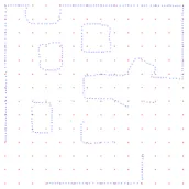
The data used to evaluate our algorithms is taken from Lenac et al. [21], where a robot’s exploration of a room was simulated using the Player-Stage software [2]. This produced a series of scan scenarios, each composed of a veriiable scan pose (x, y, rotation) and polar scan coordinates (distance, rotation) which mimic LiDar scanner data. The map of the environment (into which our algorithm will locate itself) was then calculated from these scans into a cartesian dataset, and then subsampled to a tolerance of 0.2 units such as to speed up the algorithm’s execution Figure 2. Ωe should note that the data utilised had no speciied scale: this can be estimated using the speciications of an of-the-shelf Li-Dar range inder [1].

−5 0 5

−5 0 5

X

Y

−5 0 5

−5 0 5

X

Y

−5 0 5

−5 0 5

X

Y

Figure 2: Efects of sub-sampling on features in the refer-ence map, with tolerances of 0.1, 0.2 & 0.5 units respectively.

create a consistent system accounting for the stochastic nature of genetic algorithms.

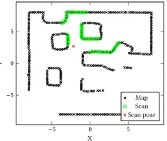
−5 0 5

−5 0 5

X

Y

Map Scan Scan pose

Figure 3: Scan 110 as located in the reference map, with pose.

4

SOLUTION EVALUATION

Ωe deine a combined error metricE=dhp× |Rh−Rr|, wheredhp

is the absolute distance between each estimated pose, andRh,Rp

are the respective rotations from North of the hypothetical and reference pose. As such, a smaller error represents a more accurate pose. This allows the outputs of our algorithms to be evaluated independently from their itness functions, and therefore allow us to compare output poses. As we are only searching for a single pose, we will only consider the best individual from each run’s inal generation as the output of an algorithm. These form the set of results for each algorithm which will be evaluated using statistics appropriate to individual experiments. An additional measure of eiciency is deined as the product of the combined error and the ex-ecution time of the algorithm, thereby allowing quicker algorithms to be precise algorithms.

5

BENCHMARK ALGORITHM

An existing GA by Robertson and Fisher [30] was adapted as a benchmark algorithm for the purpose of this project; it consists of a standard GA with incremental⁄decremental mutation,

parameter-speciic crossover (parameters are x, y,θ) and tournament based

selection. Diferent termination conditions were used: these were either generation based (maximum number of permitted iterations) or time based (maximal allowed execution time, which permits a generation to inish if it was started before the time limit). The mutation rate, crossover rate, population size and number of gener-ations were sequentially optimised for a given scan to maximise the algorithm’s performance in our test data, creating a robust bench-mark.

The itness function deined by Robertson and Fisher [30] was

inverted from a minimisation (E=Íi|Si−MI|where S is a(x,y)

point in the scan and M is S’s closest point in the map) to a

maximi-sationM=1+1E; This provides a more accentuated curve of itness

in the hope of improving the convergence capabilities of both the benchmark and new algorithm, in addition to adhering standards for GAs established by Eiben and Smith [15]. This was validated using the itness landscape in Figure 1, which corresponded to the solution pose.

Figure 4: Efects of crossover and mutation rates on the benchmark algorithm’s execution time.

Mutation and crossover probabilities were optimised for our test case (scan110) by execution the algorithm from 60 randomly gen-erated poses; the lowest average pose error (deined in section 4) was selected, resulting in a optimal parameters of CXPB=0.8 and MUTPB=0.8, as visible in Figure 4. A similar analysis was conducted using these parameters to mutation sizes, as sampled from a normal

distribution withµ = 0,σ =1.0; this was deemed to provide a

balance between the frequency in small mutations (to adequately reine the inal pose) and larger mutations (to increase the con-vergence rate of the pose from the initial pose). The optimised standard deviation of this distribution for our test scan (scan 110) was veriied by running the algorithm 30 times using previously de-ined parameters and a varying mutation size, as visible in Figure 5. Population sizes and number of generations were set to 50, such as to provide a more practical execution time which would mimick the speciications of an embedded system, whilst increasing the diiculty of the problem for all algorithms evaluated.

0.2 0.4 0.6 0.8 1 1.2 1.4 1.6 1.8 2 2.2 0

5 10 15 20

Squared variance of standard distribution of step sizes.

Combine

d

err

or

Figure 5: Efects of varied mutation sizes on performance of the benchmark algorithm.

6

ALGORITHM DESIGN

GECCO ’18, July 15–19, 2018, Kyoto, Japan

maximas. The evolutionary behaviour represented a form of elitism,

where the topnpercentile of the population was retained at each

generation and duplicated into ofspring, which increase the genetic diversity via crossover or mutation according to a set probability.

This is known at the(µ+λ)algorithm [3] [31], whereµrepresents

the number of ittest individuals to select at each generation, andλ

represents the number of ofspring to generate. The mutation rate was set to 1.0, whilst no crossover was used; this minimised the average resultant combined error by maximising the incremental movement of individuals and reduced the occurance of destruc-tive crossover. A high elitism rate of 0.95 was found to minimise the combined error when evaluated across a possible range of [0, 1]. Mutation sizes were drawn from a normal distribution with

µ =0,σ =1.05. This was deemed to provide a balance between

the frequency in small mutations (to adequately reine the inal pose) and larger mutations (to increase the convergence rate of the pose from the initial pose). The near-optimality of this distribution for our test scan (scan 110) was veriied by running the algorithm using previously deined parameters and a varying mutation size. An additional improvement of the population’s initialisation in-volved arranging individuals into a grid layout; this improved the probability that all local minimas would be explored, as the elitism rate rarely removes individuals from the population. In order to pro-vide an adequate breadth of search without a large computational overhead, we also experimented with a grid-like instantiation of individuals (see Figure 6). This enabled the algorithm to evaluate a larger number of candidate individuals, of which the top 50 are used as a primed population in the elitist algorithm previously described.

Figure 6: A grid based initial population

7

EVALUATION AGAINST BENCHMARK

These two improvements were evaluated against our benchmark GA in succession, with the latter grid-arrangement including the former elitist selection and parameters. All 3 were evaluated 30 times using optimal parameters for each algorithm, and scan110 as a representative of scans of the dataset.

7.1

Elitist selection

This found the elitist algorithm to be more precise with limited algorithmic capacity, with a mean combined error of 0.191 against 1.839. The result was validated using a two-tailed T-Test (with un-equal variance) between the set of combined errors (N=30, p¡0.01). However, the elitist algorithm also required slightly more time to run (see Table 1), which brings into question the eiciency of the algorithm.

Combined error Execution time (s)

Benchmark Elitism Benchmark Elitism

Mean 1.839 0.191 46.923 48.522

Stdev 3.151 0.478 9.160 9.057

Table 1: Combined error and execution time over 30 runs of benchmark and elitist algorithms

Further to the previous experiment, the code was modiied to loosely constrain the available execution time; this functioned by halting the algorithm if, at the end of a generation, the elapsed time was larger than a speciied threshold. As the subsequent results had non-exact execution times, the results were weighed according to their execution time, such that the statistics were ran on values representing the product of the execution time and combined error. Lower values therefore represent better eiciency in resolving the problem.

The elite algorithm was found to produce more eicient results across the set of target execution times Figure 7. This is most visible by the comparatively low median (0.550 against 12.960), along with a more eicient upper quartile (2.110 against 82.407). This demon-strates that the elite algorithm produces consistently more eicient solutions than the benchmark algorithm. Poor eiciency values still occur, as demonstrated by the large whiskers.

10−5 10−3 10−1 101 103

Elite Benchmark

Combined error×execution time

Figure 7: Performance of each algorithm with 50 population, as many generations as possible within the time frame and optimal parameters for each algorithm.

These results can be further analysed in Figure 8, where the results are bucketed by execution time. A T-Test (paired across time buckets) demonstrates the eiciency of the elitist algorithm (i.e:

lower execution time×combined error) per execution time (means

of 23.622 vs 100.865, p¡0.001, N=360). This is not the case for all time limits; benchmark runs limited to 5-10s are not signiicantly more

eicient (23.724 average combined error×execution time) than the

elite algorithm (26.231). This may be due to the benchmark GA’s use of crossovers to rapidly explore areas of the map which are not yet populated; an equivalent breadth of search is not available in our algorithm due to the small mutation sizes and lack of crossover; this does appears to disrupt the mutation-based reinement, leading to a higher error in the benchmark algorithm.

5-10 10-1515-2020-2525-3030-3535-4040-4545-5050-5555-60 >60

0 100 200 300

Real execution time (s)

Exe

cution

time

×

combine

d

err

or

Elite ef. Benchmark ef.

5-10 10-1515-2020-2525-3030-3535-4040-4545-5050-5555-60 >60

0 2 4 6

Combine

d

err

or

Elite error Benchmark error

Figure 8: Average run time×combined error for each algo-rithm, using as many generations as possible in time limit, optimal parameters for each algorithm and population of 50.

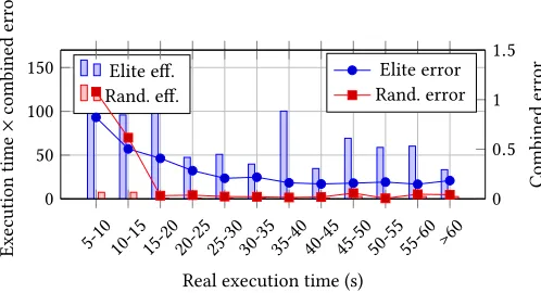
by the large upper percentiles in Figure 7). This may be due to the stochastic nature of the genetic algorithms, or more particu-larly the population initialisation, and may occur if no individual’s local maxima is the global maxima. Combining elitism with a grid-instantiation was next evaluated using the same methodology with which our algorithm was previously compared to the benchmark. The elitist algorithm including a grid-based initialisation of 200 individuals (followed by the evolution of the 50 best individuals) was executed 30 times across a range of time limits, producing the data found in Figure 9.

5-10 10-1515-2020-2525-3030-3535-4040-4545-5050-5555-60 >60

0 50 100 150

Real execution time (s)

Exe

cution

time

×

combine

d

err

or

Elite ef. Rand. ef.

5-10 10-1515-2020-2525-3030-3535-4040-4545-5050-5555-60 >60

0

0.5

1

1.5

Combine

d

err

or

Elite error Rand. error

Figure 9: Performance of grid-based initialisation compared to random instantiation, both using elitist selection.

The grid-initialised algorithm was found to be more eicient when compared to a random initialisation (T-Test paired across

bucketed real execution time, average execution time×error of

2.26 vs 69.00, p¡0.001, N=360). This is likely due to a reduction in the number of algorithm failures, where no adequate pose was found within the time limit; we would expect this to occur less frequently when sampling the map at a higher frequency and consistency. The efects of this are visualised in Figure 10, where the standard

5-10 10-1515-2020-2525-3030-3535-4040-4545-5050-5555-60 >60

0 1 2 3

Real execution time (s)

StDe

v.

of

Combine

d

err

or

Grid initialisation Random initialisation

Figure 10: Improved pose accuracy and algorithm success from grid-based initialisations compared to random initial-isation.

10−5 10−3 10−1 101 103

Grid Random Benchmark

Combined error×execution time

Figure 11: Performance of each algorithm over 30 execu-tions for various time limits.

deviations for each execution time group are generally lower for grid-based initialisation than the standard algorithm. This is found to be statistically signiicant for two thirds of the groups using an F-Test (p¡0.001), therefore demonstrating that grid-based initiali-sations greatly increase the accuracy of the algorithm. Ωe should note that optimal grid density or parameters were not explored for the map or scan, and it could therefore be possible to further accentuate the efect of this method on the output pose.

Ωe should additionally note that while the feature was envi-sioned using a grid pattern, the use of a larger initial population which is randomly distributed around the map does achieve a simi-lar performance. This was validated over 30 runs of the algorithm,

which produced a mean result (in execution time×combined error)

of 3.74 across all execution time buckets, compared to the grid-based algorithm’s mean of 2.255. A paired T-test across execution time buckets conirmed that the mean standard deviations were not statistically discernible from grid-based initialisations (N=360, p=0.295).

GECCO ’18, July 15–19, 2018, Kyoto, Japan

Grid algorithm’s results in Figure 11.

Ωe therefore demonstrate that optimisations are possible for purely genetic localisation algorithms, improving the accuracy, computational requirements and precision of our localisation within a map. The optimised algorithm has been reduced away from a volatile genetic algorithm, which beneits from crossover to explore a large map with little computational power. In it’s place, we rely on inding a reasonable initial pose estimation through a sparse brute force, before reining it through repeated mutation to ascend the itness gradient. As the mutation has a likelihood of approximately 50 % of being counter-productive (as it can move the individual towards or away from the optima), it stands out as a signiicant ineiciency in the algorithm, leading us to a necessary comparison with a gradient ascent algorithm, which we will design and evaluate in section 8.

8

ICP ALGORITHM DESIGN & EVALUATION

Given the lack of comparison between genetic algorithm and recent classical algorithms, an additional experiment was undertaken to help highlight ineiciencies in the pose reinement of GAs. Follow-ing Yang et al. [34]’s implementation of a Branch-and-Bound & ICP algorithm, an ICP implementation [18] was adapted for use with our grid-layout algorithm. This aimed to form a representative algorithm from the non-genetic research, and preliminary results signiied that further optimisation was not required to demonstrate the beneits of this approach. Following Censi et al. [8], who states that it would be possible to apply a ’classical’ algorithm to a global pose localisation problem by running it from a number of random poses, the algorithm functioned by applying the ICP algorithm from 200 hypothetical poses laid across a grid on the map, using the same grid pattern and density as the Grid-GA. The previously deined combined error metric (see section 4) is then used to se-lect the inal pose estimation from the set of ICP-reined candidate poses. The reinement of candidate poses was executed in parallel using the same compute cluster as in our grid-based GA, thereby utilising an equally maximal amount of concurrency equivalent to our GAs parallel evaluation of individuals. The algorithm was run 360 times to create a dataset of comparable size to the grid-based algorithm’s dataset (which was created using 30 runs over 12 target durations). As visualised in Figure 12, the grid-ICP has a similar median eiciency to the grid-based GA (medians: Grid-GA = 0.73, Grid-ICP = 1.33), but is much more consistent. This is demonstrated by the standard deviation lower standard deviation of 7.760 for the Grid-ICP, compared to 68.63 for the Grid-GA. Ωe should note that whilst Figure 12 displays a similar spread of data using interquar-tile ranges, we decided to comparatively evaluate the eiciency of the algorithms using the standard deviation as we have previously decided not to exclude outliers. As the IQR is ’padded’ against out-lying values, it is not representative of the worst case values seen in the overlow bin of Figure 13, demonstrating why the Grid-ICP algorithm is more consistent than the Grid-GA.

A paired T-Test across the pose error×execution time results

for ICP and the grid-initialised algorithms found the means to be statistically diferent (N=360, p¡0.01). This indicates that the GA based algorithm is indeed more eicient, with a mean eiciency of

10−3 10−2 10−1 100 101 102

Grid-GA Grid-ICP

Combined error×execution time

Figure 12: Performance of each algorithm over 30 execu-tions for 12 time limits (note logarithmic x axis)

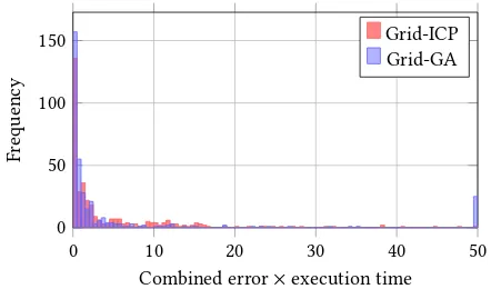
0 10 20 30 40 50

0 50 100 150

Combined error×execution time

Fr

equency

Grid-ICP Grid-GA

Figure 13: Histogram comparing the eiciency of Grid-ICP and Grid-GA algorithms

2.247 against the Grid-ICP’s mean of 4.350. Ωe further found the grid-ICP algorithm to have a much smaller mean execution time compared to the grid-GA: (3.66s, compared to 38.20s)

9

EXPERIMENTAL SUMMARY & DISCUSSION

Ωe therefore demonstrate improvements to the application of GAs to the problem of indoor localisation; these are the application of

the(µ+λ)algorithm, and priming the algorithm with a larger initial

population. These improvements highlight the inefectiveness of GAs to the problem of indoor localisation, as an unreined classi-cal algorithm can be prototyped to not only indistinguishly match the precision and eiciency of the algorithm, but would also be more suitable to an embedded application due to it’s smaller execu-tion time. Further improvements to the ICP algorithm (such as the mbICP or trICP algorithms) could further reduce the computational power requirement, as would the optimisation of grid arrangements and population density. Ωe hypothesise that this improvement is possible due to the destructive nature of the crossover operator when dealing with co-dependent parameters (as is our case), and the inability of mutations to rapidly evolve individuals in a reliable fashion without being less eicient than random walking. Both the grid-GA and grid-ICP rely on the position of at least one individual in the ’itness well’ of the global maxima, signifying that limita-tions may arise in large maps which cannot be adequately sampled through a large initial population (or to run the ICP algorithm from a dense grid).

parameters to maximally optimise an algorithm. This was the cho-sen methodology for practical reasons, as a multi-parameter search would require inaccessible amounts of computation power. Re-search in meta-genomic by Brain and Addicoat [6] suggests that it could be possible to use a genetic algorithm to optimise our GAs for a given set of scans and a map. This would improve the con-vergence speed of the candidate solutions, thereby reducing the computational time required to run the algorithm. This is not a fea-sibly rapid solution given available resources due to the stochastic behaviour of genetic algorithms and the long execution time of our algorithms.

Furthermore, the assumption of a single, smooth and global max-ima is central to the function of both grid-based algorithms. The lack of common test-benches (as opposed to other ields such as IRIS dataset in computer vision [16]) further complicates the task of comparing algorithms in generalisable cases. As demonstrated in our landscapes in Figure 1, this is the case for our test scans and maps. However, if exploring a repeated environment where features occur with slight variations (for example oices with desks, cabinets, walls), both the Grid-ICP algorithm and grid-pattern al-gorithm may converge to an incorrect maxima; depending on the density of the initial grid and the location of individuals within the local topology of the maxima. The inability to later explore areas which are not sampled in the initial population through large muta-tions or crossovers would prevent either algorithm from searching unexplored areas, causing the algorithms to become stuck in the local maxima and return an incorrect pose.

Therefore, we could hypothesise that feature dense search spaces with associated mountainous itness landscapes could be better explored by more volatile implementations of GAs, such as the al-gorithms proposed by Robertson and Fisher [30] or Lenac et al. [20], with additional reinement using a classical algorithm (as proposed by Lenac et al. [21]). Such maps could be caused by either having a poorly featured scan dataset (due to low sensor range relative to map size). Nevertheless, we should note that the use of a single test case proves no guarantee of any form of dominance between algorithms, and that although we postulate that non-smooth it-ness landscapes are infeasible given our current itit-ness metric, the existence of these would form an edge case to our current analysis. Therefore, whilst purely elitist genetic algorithms are inefective in our test case, a crossover operator may be necessary to explore larger maps; this would also preclude requirement of a short com-putation time due to the added complexity.

The lack of exploration of the solution space’s topology is there-fore both an unexplored and central issue to the problem of in-door localisation through GAs; this draws a strong comparison to Mitchell [27]’s statement that "GAs are most applicable in non-smooth, non-unimodal search spaces".

Ωe should note that the indings presented here depend on an underlying assumption; the presence of a smooth itness landscape, which we can sample with suicient density to allow for random walking to propagate a candidate pose to the global maxima. Ωe may expect these to exist in the context of indoor localisation as feature-dense reference maps, but this amounts to a iner resolution of the current problem, requiring a higher sampling density and computational power but remaining equally solvable. Furthermore, Grefenstette [17] states that "If [a search] space is well understood

and contains structure that can be exploited by special purpose search techniques, the use of genetic algorithms is generally com-putationally less eicient".

Ωe conclude that whilst it is possible to optimise GAs for a par-ticular map topology and scan, the application of a purely genetic algorithm to the problem of indoor localisation is likely to be in-ferior in accuracy and execution time when compared to a hybrid algorithm capable of global search and gradient-ascending local re-inement (such as [34]). This is likely due to the low dimensionality of the problem, which results in a topographically unimodal itness landscape. The scope of these indings are limited to purely genetic algorithms, as hybrid genetic algorithms can avoid the diiculty of balancing exploration and exploitation through the use of alternate reinement algorithms [21] or modiications to the behaviour of the GA [9]. These may prove to be extremely beneicial when perform-ing localisation in very large spaces with limited computational capabilities, but further research should be undertaken to com-paratively evaluate the behaviours of GAs in these environments against other leading algorithms. The lack of any application of itness landscape topology to the problem precludes the possibility of asserting any dominance of GA or non-GA algorithms, but, if evaluated against a robust & diverse test bench, could allow the selection of a hypothetically optimal problem for a given scenario. Such work may result from the application of explanatory land-scape analysis to indoor localisation, as discussed in Mitchell et al. [28] and more recently Mersmann et al. [26].

ACKNOWLEDGMENTS

REFERENCES

[1] [n. d.]. LIDAR-Lite 3 Laser Rangeinder. http:⁄⁄www.robotshop.com⁄uk⁄ lidar-lite-3-laser-rangeinder.html. ([n. d.]). Accessed: 2017-4-6.

[2] [n. d.]. Player Project. http:⁄⁄playerstage.sourceforge.net⁄. ([n. d.]). Accessed: 2017-4-28.

[3] Back, T and Fogel, D B and Michalewicz, T. [n. d.].Evolutionary Computation 1 Basic Algorithms and Operators. IOP Publishing Ltd.

[4] P J Besl and H D McKay. 1992. A method for registration of 3-D shapes.IEEE Trans. Pattern Anal. Mach. Intell.14, 2 (Feb. 1992), 239ś256.

[5] P Biber and Ω Strasser. 2003. The normal distributions transform: a new ap-proach to laser scan matching. InIntelligent Robots and Systems, 2003. (IROS 2003). Proceedings. 2003 IEEE/RSJ International Conference on, Vol. 3. 2743ś2748 vol.3. [6] Zoe E Brain and Matthew A Addicoat. 2011. Optimization of a genetic algorithm

for searching molecular conformer space.J. Chem. Phys.135, 17 (7 Nov. 2011). [7] K Brunnstrom and A J Stoddart. 1996. Genetic algorithms for free-form surface

matching. InProceedings of 13th International Conference on Pattern Recognition, Vol. 4. 689ś693 vol.4.

[8] A Censi, L Iocchi, and G Grisetti. 2005. Scan Matching in the Hough Domain. In

Proceedings of the 2005 IEEE International Conference on Robotics and Automation. 2739ś2744.

[9] Chi Kin Chow, Hung Tat Tsui, and Tong Lee. 2004. Surface registration using a dynamic genetic algorithm.Pattern Recognit.37, 1 (2004), 105ś117.

[10] Kalyanmoy Deb David E. Goldberg. 1991. A comparative analysis of selection schemes used in genetic algorithms. InFoundations of Genetic Algorithms. [11] A Diosi and L Kleeman. 2005. Laser scan matching in polar coordinates with

application to SLAM. In2005 IEEE/RSJ International Conference on Intelligent Robots and Systems. 3317ś3322.

[12] F A Donoso, K J Austin, and P R McAree. 2017. How do ICP variants perform when used for scan matching terrain point clouds?Rob. Auton. Syst.87 (2017), 147ś161.

[13] F Donoso-Aguirre, J-P Bustos-Salas, Miguel Torres-Torriti, and Andres Guesalaga. 2008. Mobile robot localization using the Hausdorf distance.Robotica26, 02 (2008), 129ś141.

[14] D Ω Eggert, A Lorusso, and R B Fisher. 1997. Estimating 3-D rigid body transfor-mations: a comparison of four major algorithms.Mach. Vis. Appl.9, 5-6 (1 March 1997), 272ś290.

GECCO ’18, July 15–19, 2018, Kyoto, Japan

[16] R. A. FISHER. 1936. THE USE OF MULTIPLE MEASUREMENTS IN TAXONOMIC PROBLEMS.Annals of Eugenics7, 2 (1936), 179ś188. https:⁄⁄doi.org⁄10.1111⁄j. 1469-1809.1936.tb02137.x

[17] John J Grefenstette. 2012.Genetic Algorithms for Machine Learning. Springer Science & Business Media. 351 pages.

[18] R Harry. [n. d.]. Iterative Closest Point (ICP) implementa-tion on python. http:⁄⁄stackoverlow.com⁄questions⁄20120384⁄ iterative-closest-point-icp-implementation-on-python. ([n. d.]). Accessed: 2017-4-12.

[19] Jaromir Konecny, Michal Prauzek, Pavel Kromer, and Petr Musilek. 2016. Novel Point-to-Point Scan Matching Algorithm Based on Cross-Correlation.Mobile Information Systems2016 (24 April 2016).

[20] Kristijan Lenac, Enzo Mumolo, and Massimiliano Nolich. 2007. Fast Genetic Scan Matching Using Corresponding Point Measurements in Mobile Robotics. In

Applications of Evolutionary Computing. Springer Berlin Heidelberg, 375ś382. [21] Kristijan Lenac, Enzo Mumolo, and Massimiliano Nolich. 2011. Robust and

Accurate Genetic Scan Matching Algorithm for Robotic Navigation. InIntelligent Robotics and Applications (Lecture Notes in Computer Science), Sabina Jeschke, Honghai Liu, and Daniel Schilberg (Eds.). Springer Berlin Heidelberg, 584ś593. [22] Evgeny Lomonosov, Dmitry Chetverikov, and Anikó Ekárt. 2006. Pre-registration of arbitrarily oriented 3D surfaces using a genetic algorithm.Pattern Recognit. Lett.27, 11 (2006), 1201ś1208.

[23] Feng Lu and Evangelos Milios. 1997. Robot Pose Estimation in Unknown Envi-ronments by Matching 2D Range Scans.J. Intell. Rob. Syst.18, 3 (1 March 1997), 249ś275.

[24] Jorge L Martínez, Javier González, Jesús Morales, Anthony Mandow, and Alfonso J García-Cerezo. 2006. Mobile robot motion estimation by 2D scan matching with genetic and iterative closest point algorithms.J. Field Robotics23, 1 (1 Jan. 2006), 21ś34.

[25] T Masuda, K Sakaue, and N Yokoya. 1996. Registration and integration of multiple range images for 3-D model construction. InProceedings of 13th International Conference on Pattern Recognition, Vol. 1. 879ś883 vol.1.

[26] Olaf Mersmann, Bernd Bischl, Heike Trautmann, Mike Preuss, Claus Ωeihs, and Günter Rudolph. 2011. Exploratory Landscape Analysis. InProceedings of the 13th Annual Conference on Genetic and Evolutionary Computation (GECCO ’11). ACM, New York, NY, USA, 829ś836.

[27] Melanie Mitchell. 1998.An Introduction to Genetic Algorithms. MIT Press, Cam-bridge, MA, USA.

[28] M Mitchell, S Forrest, and J H Holland. 1992. The royal road for genetic algorithms: Fitness landscapes and GA performance.Proceedings of the irst(1992). [29] F Pourraz and J L Crowley. 1999. Continuity properties of the appearance manifold

for mobile robot position estimation.IEEE Workshop on Perception for Mobile âĂę

(1999).

[30] Craig Robertson and Robert B Fisher. 2002. Parallel Evolutionary Registration of Range Data.Comput. Vis. Image Underst.87, 1 (1 July 2002), 39ś50.

[31] Stuart C Shapiro. 1992.Encyclopedia of Artiicial Intelligence(2 volume set edition ed.). Ωiley.

[32] David A Simon. 1996.Fast and accurate shape-based registration. Ph.D. Disserta-tion. Carnegie Mellon University Pittsburgh.

[33] S Ωeik. 1997. Registration of 3-D partial surface models using luminance and depth information. InProceedings. International Conference on Recent Advances in 3-D Digital Imaging and Modeling (Cat. No.97TB100134). 93ś100.

[34] J Yang, H Li, and Y Jia. 2013. Go-ICP: Solving 3D Registration Eiciently and Globally Optimally. In2013 IEEE International Conference on Computer Vision. 1457ś1464.