Retrieving secondary forest aboveground biomass from polarimetric ALOS-2 PALSAR-2 data in the Brazilian Amazon

polarimetric ALOS-2 PALSAR-2 data in the Brazilian Amazon

.

White Rose Research Online URL for this paper:

http://eprints.whiterose.ac.uk/142130/

Version: Published Version

Article:

Cassol, H.L.G., Carreiras, J.M.D.B. orcid.org/0000-0003-2737-9420, Moraes, E.C. et al. (4

more authors) (2018) Retrieving secondary forest aboveground biomass from polarimetric

ALOS-2 PALSAR-2 data in the Brazilian Amazon. Remote Sensing, 11 (1). 59. ISSN

2072-4292

https://doi.org/10.3390/rs11010059

eprints@whiterose.ac.uk https://eprints.whiterose.ac.uk/

Reuse

This article is distributed under the terms of the Creative Commons Attribution (CC BY) licence. This licence allows you to distribute, remix, tweak, and build upon the work, even commercially, as long as you credit the authors for the original work. More information and the full terms of the licence here:

https://creativecommons.org/licenses/

Takedown

If you consider content in White Rose Research Online to be in breach of UK law, please notify us by

Article

Retrieving Secondary Forest Aboveground Biomass

from Polarimetric ALOS-2 PALSAR-2 Data in the

Brazilian Amazon

Henrique Luis Godinho Cassol1,* , Joã_{o Manuel de Brito Carreiras}2 _{, Elisabete Caria Moraes}1_,

Luiz Eduardo Oliveira e Cruz de Aragã_o1,3_{, Camila Val}é_{ria de Jesus Silva}4 _{, Shaun Quegan}2 and Yosio Edemir Shimabukuro1

1 _{National Institute for Space Research (INPE)—Remote Sensing Division, Av. dos Astronautas 1758, Jd}

Granja, Sã_{o Jos}é_{dos Campos, S}ã_{o Paulo 12227-010, Brazil; bete@ltid.inpe.br (E.C.M.);}

laragao@dsr.inpe.br (L.E.O.e.C.d.A.); yosio@dsr.inpe.br (Y.E.S.)

2 _{National Centre for Earth Observation (NCEO), University of Sheffield, Western Bank, Sheffield S10 2TN,}

UK; j.carreiras@sheffield.ac.uk (J.M.d.B.C.); S.Quegan@shef.ac.uk (S.Q.)

3 _{College of Life and Environmental Sciences, University of Exeter, Exeter EX4 4RJ, UK}

4 _{Lancaster Environment Centre, Lancaster University, Lancaster LA1 4YQ, UK; camilaflorestal@gmail.com}

* Correspondence: henrique@dsr.inpe.br; Tel.: +55-12-3208-6458

Received: 25 October 2018; Accepted: 30 November 2018; Published: 29 December 2018

Abstract:Secondary forests (SF) are important carbon sinks, removing CO2from the atmosphere

through the photosynthesis process and storing photosynthates in their aboveground live biomass (AGB). This process occurring at large-scales partially counteracts C emissions from land-use change, playing, hence, an important role in the global carbon cycle. The absorption rates of carbon in these forests depend on forest physiology, controlled by environmental and climatic conditions, as well as on the past land use, which is rarely considered for retrieving AGB from remotely sensed data. In this context, the main goal of this study is to evaluate the potential of polarimetric (quad-pol) ALOS-2 PALSAR-2 data for estimating AGB in a SF area. Land-use was assessed through Landsat time-series to extract the SF age, period of active land-use (PALU), and frequency of clear cuts (FC) to randomly select the SF plots. A chronosequence of 42 SF plots ranging 3–28 years (20 ha) near the Tapajós National Forest in Parástate was surveyed to quantifying AGB growth. The quad-pol data was explored by testing two regression methods, including non-linear (NL) and multiple linear regression models (MLR). We also evaluated the influence of the past land-use in the retrieving AGB through correlation analysis. The results showed that the biophysical variables were positively correlated with the volumetric scattering, meaning that SF areas presented greater volumetric scattering contribution with increasing forest age. Mean diameter, mean tree height, basal area, species density, and AGB were significant and had the highest Pearson coefficients with the Cloude decomposition (λ3), which in turn, refers to the volumetric contribution backscattering from cross-polarization (HV) (ρ= 0.57–0.66,

p-value < 0.001). On the other hand, the historical use (PALU and FC) showed the highest correlation with angular decompositions, being the Touzi target phase angle the highest correlation (Φ_{s) (}ρ= 0.37 andρ= 0.38, respectively). The combination of multiple prediction variables with MLR improved the AGB estimation by 70% comparing to the NL model (R2adj. = 0.51; RMSE = 38.7 Mg ha−1) bias = 2.1 ±37.9 Mg ha−1 by incorporate the angular decompositions, related to historical use, and the contribution volumetric scattering, related to forest structure, in the model. The MLR uses six variables, whose selected polarimetric attributes were strongly related with different structural parameters such as the mean forest diameter, basal area, and the mean forest tree height, and not with the AGB as was expected. The uncertainty was estimated to be 18.6% considered all methodological steps of the MLR model. This approach helped us to better understand the relationship between parameters derived from SAR data and the forest structure and its relation to the growth of the secondary forest after deforestation events.

Keywords: backscattering; L-band; SAR polarimetry; microwave; Chapman-Richards model; tropical forest

1. Introduction

Secondary forests (SFs) are defined as areas of forests where clear cut was made only by anthropic actions, whether or not for conversion to other land uses, according to the Convention on Biological Diversity (CDB) [1]. Despite the multiple definitions of SFs found in the literature [2–5], hereafter, we consider as SFs areas that are in a process of regeneration after complete removal of primary forests (PFs) through clear cut or areas with characteristics in conformity with the definition proposed by the CDB [1]. This definition was chosen because it adequately encompasses the classes of SF discriminated by satellite data on a regional or global scale [6].

According to Forest Resources Assessment FRA/FAO [7], from 106 nations located in the tropics, 36 have all remaining forests composed of SFs, almost half of all tropical countries have the majority of their forest land dominated by SFs, and only 19 of them have the dominance of PF in their territory, including Brazil. These numbers have led some authors to recognize the importance of SFs, not only because of the capacity of these forests in maintaining biodiversity and mitigating anthropogenic carbon emissions, but also because SFs are likely to be the dominant state of rainforests in the future [2,8–12].

Forests undergoing regeneration partially offset carbon emissions from land use change and fossil fuels by accumulating carbon in their biomass. It has been estimated that SFs have the potential to accumulate 0.86 Pg C year−1in Latin America [10]. This value is twice as large as carbon emissions from land-use, land-use change, and forestry (LULUCF), which accounts for 0.47 Pg C year−1[13]. In the Brazilian Amazon, estimates of C accumulation in SFs vary between 0.06 Pg C year−1and 0.15 Pg C year−1[14,15]. Despite large uncertainties in these estimates, carbon uptake by SFs is likely to represent 17–44% of total carbon emission from deforestation in the Brazilian Amazon. To improve these estimates, it is therefore crucial to accurately quantify the extent and growth rates of SFs in the Amazonia [10,13,15,16]. For instance, the mean annual increment (MAI) of the aboveground biomass (AGB) varies from 0.16 Mg ha−1 year−1 to 30 Mg ha−1year−1throughout the Brazilian Amazon, with higher growth rates in the central Amazon (dry season < 4 months 100 mm rainfall) than in the eastern Amazon (dry season_≥4 months) regardless of the previous land-use [17–21]. Furthermore, the intensity of the previous land-use reduces about 35% of the MAI (7.45 Mg ha−1year−1) in areas subjected to pasture and agricultural practices and about 40% (8.05 Mg ha−1year−1) if the frequency of clear cuts are greater than twice, when compared to SFs areas with previous “light” land use [18,19,22–26].

Secondary forests covered between 140,000 km2 and 228,000 km2until 2010 in the Brazilian Amazon [27–29], representing approximately 30% of accumulated deforestation since 1988 (PRODES/INPE) [30]. The estimation of the extent of the SF is often made using data from optical sensors [31,32]. However, the low ability of these sensors in separating succession classes, confusion with other vegetation classes, and the persistence of rain clouds may reduce the accuracy of these estimates in the tropical regions [33,34]. To overcome these problems, the analysis of time-series of land cover maps is essential for mapping SFs to avoid misclassification in the tropics [27]. These time-series also provide relevant information about prior land-use history of each SF patch, including the period and type of land-use before abandonment, the clear-cut frequency, and the fire history [27,28,34,35]. This multi-temporal information is useful to model SF growth rates and to reduce the uncertainty of estimates throughout the Amazon region [26,36].

AGB is usually estimated through regression models based on empirical relationships between AGB and radar parameters, including backscattering intensity or polarimetric decompositions [37,38,41,42]. L-band SAR data is currently being used for AGB modeling, as the wavelength of its microwave pulse (23.5 cm) matches the dimensions of forest woody components, as twigs, secondary branches, and even the stems in the initial secondary successions. However, the sensitivity of L-band SAR data for estimating AGB is efficient until 100–150 Mg ha−1, with saturation of the signal observed above these values [39]. To surpass this limitation, the use of multiple variables obtained from polarimetric decomposition has been proposed to describe these structurally complex environments [37,43–46]. Multiple linear regression (MLR) have achieved R2= 0.44 (RMSE = 54.32 Mg ha−1) for AGB prediction (100–450 Mg ha−1) in the secondary and primary forests of the Tapajó_{s National Forest, Brazilian}

Amazon, using multiple variables from L-band (ALOS PALSAR) [37]. The best prediction variables were the Touzi helicity, the Freeman–Durden volumetric scattering, and the Cloude anisotropy, along with slope and elevation aspects from the digital elevation model [37]. Santos et al. [45] observed a R2_{= 0.75 (RMSE = 29 Mg ha}−1_{) at the same study site by adding the TanDEM-X interferometry in}

the MLR model. The best MLR model has two prediction variables: interferometric coherenceγ_i

from TanDEM-X and the Freeman–Durden volumetric scattering Pvfrom ALOS L-band. Although

these studies have retrieved AGB using polarimetric data, they were carried out only on PFs or using logarithmic models. Therefore, the potential of polarimetric data for assessing AGB in the SFs is still rare in the literature.

Hence, the main goal of this paper is to retrieve the aboveground biomass for secondary forests across the Santarém study site by exploring polarimetric (quad-pol) data from the Advanced Land Observing Satellite-2 Phased Array L-band SAR-2 (ALOS-2 PALSAR-2). We tested two regression models commonly used in the literature: nonlinear regression (NL) and multiple linear regressions (MLR). Second, our objective is to evaluate the quad-pol data to characterize SFs according to past land-use, assessed through Landsat time-series classification to understand how the SAR parameters are related to forest regrowth pathways. It is expected that land-use history influences the relationship between the polarimetric decompositions (SAR data) and the biophysical variables (forest structure) and, from this, the accuracy for estimating AGB stock and dynamics can be substantially improved.

2. Materials and Methods

The study was carried out at the vicinity of the Tapajós National Forest (FLONA Tapajós), hereafter described as the Santaré_{m site, located 80 km south of the city of Santar}é_{m, Par}á_state.

This site comprises an area of 1.118 km2and was part of the REGROWTH-BR project, whose objective was to study SFs of varied ages and subjected to different historical land-use [28] (Figure1).

2.1. A Brief History of the Land-Use in the Santarém Region

Santarém has a long tradition in the production of raw materials from agriculture to forest extractivism [47]. Archaeological discoveries in this region showed continuous human activities that date back to 7000–8000 years [48]. When the Europeans arrived in Santaré_{m in the 17th century,}

the region was already a complex center with a structure formed by several indigenous nuclei that practiced agriculture, trade, and taxation [48].

2.2. Site Description

The climate is classified as Am by Köppen climatic definition, with mean annual temperature between 25.5 and 26.7◦C [51,52]. According to Chave et al. [53], Santaré_{m site is considered moist}

forest located in areas with annual rainfall between 1500 and 2500 mm and dry season length <5 months. The dry season, considering average monthly rainfall lower than 100 mm, occur from July to November. The soils are predominantly Oxisols (red-yellow Latosols), with low cation exchange capacity, high saturation by exchangeable aluminum Al+++, low pH, and are mainly found in non-flooded upland Terra-firme areas [54]. In a lesser proportion than Oxisols, Ultisols (Argisols) occurs in lowland and floodplain areas, which are also nutrient poor and often sandier [55–57]. The terrain is flat to undulate and the altitude is 100 m above sea level [58].

Figure 1. Site location and field plots (crosses) inside the Regrowth-BR project (red box) and the location of the Large-Scale Biosphere–Atmosphere Experiment in Amazonia (LBA) in green dot. Background image is ALOS-2 PALSAR-2 color composite of Yamaguchi three scattering mechanisms: RGB/odd-bounce (Odd), volumetric (Vol.), and double-bounce (Dbl.). Red continuous line represents BR-163 highway, which connects city of Santaré_{m, Par}á_{State, and Cuiab}á_{, Mato Grosso State. Optical}

background image is Landsat 5 TM Path/Row 227/69 of 29 June 2010, RGB/short-infrared (band 5), near-infrared (band 4), and visible red (band 3).

Terra-firmepresents a bi-modal distribution of tree-canopy height, one stratum formed by emergent trees asManilkara huberi(Ducke) Chev. (Maçaranduba) andHymanaea courbarilL. (Jatobá) with an average height of 35–40 m and a lower stratum made of sub-dominant trees (average height = 15–30 m) [60–62]. The SFs, however, show a unimodal distribution of tree-height with mean 14.3 m where emergent trees are rare and represented by small individuals [63]. The species density ranged between 133 and 186 sp ha−1, and the tree density is 441±43 ind ha−1with the most prominent families being Lechytidaceae and Fabaceae [51,60,61].

2.3. Field and Satellite Imagery Data

The processing steps of field inventory and ALOS-2 PALSAR-2 data are shown in Figure2and are described in the following sections.

Figure 2.Methodological flowchart. Land use history of secondary forests (SFs) was obtained from the analysis of Landsat time-series [28], whereby were extracted the SF age, the period of active land use (PALU), the frequency of clear cuts (FC). Field data processing following forest inventory to obtain biophysical variables of SFs is highlighted in green. In yellow, we summarize the processing steps of full-polarimetric SAR data. The methodology to characterize and to model AGB in SFs is shown in the middle panel. Dashed boxes represent statistical analysis.

Field plot data were composed by two databases: 16 plots measured in this study and 26 plots measured by Silva [64] (Table1). The sample plots were placed close to the FLONA of Tapajós on either side of the BR-163 highway, 100 km to the south of the city of Santaré_{m (Figure1).}

a DBH≥10 cm were measured in a 20 m×100 m plot size, and trees with a DBH≥20 cm were measured in a 60 m×100 m plot size.

Table 1.Field plot information by age, diameter at breast height (DBH at 1.3 m height), inventory date, succession class, area, and plot size.

N Plot Size (m)

DBH min (cm)

Age (Years)

Inventory Date

(Year) Succession

Area

(ha) Reference

16 10×100 5 16–28 2015 Advanced (Adv) 1.60 Our study 16 20_×100 10 16–28 2015 Advanced (Adv) 3.20 Our study 16 60_×100 20 16–28 2015 Advanced (Adv) 9.60 Our study 14 20_×50 5 1–7 2012/13 Initial (ISS) 1.75 Silva et al. [64]

9 20×50 5 7–16 2012/13 Intermediate (IntSS) 2.40 Silva et al. [64] 3 25×100 10 >16 2012/13 Advanced (Adv) 1.35 Silva et al. [64]

Silva [64] carried out a field campaign between 2012 and 2013 at the same site (Table 1). The method consisted of the collection of 23 plots (20 m×50 m) for the SF with initial secondary succession (ISS) and intermediate secondary succession (IntSS), and three plots for the advanced SF (25 m×100 m). In both databases, all individuals were identified at the species level.

2.4. Aboveground Biomass (AGB) Allometric Equations

The total AGB is composed by the sum of three components of the forest plots: the living tree AGB, the palm AGB, and the standing dead tree AGB. Each of these components was addressed separately and has their own allometric equations for AGB estimation. The total AGB, hereafter named AGB, was then extrapolated to unit area (Mg ha−1).

We evaluated 23 allometric equations to estimate AGB that are available from the literature for primary and secondary forests, and compared the equations’ estimates with those from 148 harvested trees [65,66]. All tested equations underestimated AGB, but the equation from Brown et al. [67] presented the lowest relative root mean square error (RMSE = 14%, obtained by the ratio between the RMSE and the average observed AGB). The underestimation was due to the errors concerning individuals with DBH 30 cm whose values were superior to 400 kg and to the high number of PFs species in the harvested trees. Hence, living AGB was estimated with the equation developed by Brown et al. [67] (1)

AGBlive =exp

−2.41+0.9522 lnDBH2hρ (1)

where AGB is the live aboveground biomass in kg, DBH in cm, h is the total height estimated by hypsometric equations adjusted by ecological species groups by Cassol et al. [63], and ρ (rho) is the wood density collected from the literature and from the Global Wood Density Database [63,68]. Palm AGB was measured with distinct equations according to Table S1, Supplementary Materials.

The AGB of standing dead trees was estimated with Equation (1) using a rotten wood density

ρ= 0.342 g cm−3and with the equations in the Table S1, Supplementary Materials for dead palms usingρ= 0.327 g cm−3[69].

The SF plots provided by Silva et al. 2016 had their AGB estimated by Uhl equation [18] (2)

AGBlive =exp

−2.17+1.02 lnDBH2+0.39 ln(h) (2)

2.5. Growth Models for Biophysical Variables

the basal area (G), the tree density (N), the species richness (S) and the aboveground biomass (AGB). The selected growth yield model was Chapman-Richards (8) as [70] (3)

Yt=A

1−e−ktc+ε (3)

where Yt represents the size of the variable at age t; A refers to the asymptote (maximum value of Y when the age tends to the infinite), the coefficient k is the growth rate of Y as a function of time t, c is the shape of the curve (inflection point), andεis the experimental error. The negative exponential was used to estimate N (4) as [25]

N=Na+ (N0−Na)e−kt+ε (4)

where N0 is the asymptote (tree density per hectare at t = 0), Na is the tree density per hectare at

t =∞_{, k is the decrease rate of N at time t. The parameters of the (3) and (4) were adjusted using the}

non-linear least squares method [71].

The input data for the growth models were obtained from SFs data located in Santarém region with ages varying from 1 to 30 years [72–74], along with the field plots measured in the present study. Plots obtained from these studies vary according to size, age, and methodology of measurement, but were carried out under similar environmental conditions (same geographic location)—first model assumption. However, the high variability of the dataset may result in the non-convergence of the growth model parameters; and a simple solution is to hold fixed each one of the model parameters, usually the asymptote [75]. Thus, we assumed that the asymptote (A, N, or N0) of each

biophysical parameter of the SF resembles the values of adjacent PF—second model assumption [25]. These maximum values were obtained from the literature and correspond to the mean value observed in the PFs located nearby the study area (Table2). In this scope, were considered as PFs the forests that have never been clear cut in the Landsat time-series, according to the references of the Table2. The goodness-of-fit of the Chapman-Richards models was evaluated according to the significance and the confidence interval of their parameters. Moreover, a visual analysis of their residuals was performed [76,77].

From the adjusted models, the accumulation rates of the biophysical variables were obtained through the partial derivatives of the growth curves. The mean annual increment (MAI) was obtained by the derivative of the second order, or simply by dividing the estimated value by the corresponding age [78]. The age at which SF growth rate is maximum (maximum MAI) was then estimated according to the MAI curves.

Table 2.Asymptote of the biophysical variables in the primary forest used for modeling the secondary forest growth.

Biophysical Variables Asymptote Units References

Mean diameter (DBH) 23.1 cm [25,58,79–84]

Mean total tree height (Ht) 25.0 m [25,79,82,85,86]

Basal area (G) 24.4 m2_ha−1 _{[25,79,82,85,87–91]}

Species richness (S) 133.00 sp ha−1 [60]

Tree density (N) 433.00 individuals ha−1 [25,60,80,82,88,90,91] Aboveground biomass (ABG) 314.00 Mg ha−1 [25,60,61,79,92]

2.6. Landsat Time-Series Classification

(W m−2sr−1µm−1); then they were calibrated to top of atmosphere (TOA) reflectance using calibration factors and equations provided by Chander et al. [94].

This time-series of land cover maps was extended to the period 2005–2010 and image classification of Landsat imagery was done with a machine learning algorithm (random forests) by Carreiras et al. [28]. The time-series were updated by visual interpretation only in the place where the sample plots were allocated.

Table 3.Landsat 5 Thematic Mapper (TM) and Landsat 7 Enhanced TM plus (ETM+) data acquired over the Santarém site (Path 227, Row 62).

Date Sensor Date Sensor Date Sensor

24 August 1984 TM 20 October 1993 TM 29 August 2003 TM

26 July 1985 TM 10 October 1995 TM 1 July 2005 TM

29 July 1986 TM 25 August 1996 TM 5 August 2006 TM

16 July 1987 TM 27 July 1997 TM 21 June 2007 TM

3 August 1988 TM 15 August 1998 TM 30 November 2008 TM

22 August 1989 TM 3 September 1999 TM 12 July 2009 TM

9 August 1990 TM 5 September 2000 TM 29 June 2010 TM

11 July 1991 TM 16 September 2001 ETM+

Landsat time-series were used to extract the land-use history in SFs, such as the age, the period of active land-use (PALU), and the frequency of cuts (FC), according to methodology described in Carreiras et al. [28]. The SF age was defined by age since the last deforestation event, PALU is the period of active land use for agriculture or livestock practices, in years, and FC is the number of deforestation events (clear cut events).

2.7. ALOS-2 PALSAR-2 Data Processing

Two quad-pol scenes covering the study site were acquired in CEOS SAR format Single Look Complex (SLC) at processing level 1.1 in slant range and HBQ mode of acquisition (high sensitivity). SAR images were acquired at descending orbit in a right-looking off nadir angle (θ) of 28–31◦. The SLC nominal resolution is 2.86 m and 3.13 m in range and azimuth respectively. Both scenes were acquired at the end of rainy season (6 February 2015) (Table S2, Supplementary Materials).

The cumulative rainfall on the date of acquisition and the day before was 10 mm [95]. The low accumulated precipitation at the previous date, however, should not cause major problems related to the increase in dielectric constant given the high evaporation in this season (about 3.5 mm day−1_),

which partially cancels the cumulative rainfall.

In orbital low-frequency SAR systems, the path of the microwave pulse traverses twice the ionosphere, a region of free electrons pervaded by the magnetosphere resulting in the rotation of the plane of the polarization wave, known as Faraday rotation (FR) [96]. The magnitude of the FR depends on a number of factors, including RADAR wavelength, degree of ionization, solar activity, geographic position, and total electron content (TEC) at the acquisition date. The TEC is defined as the amount of free electrons in the ionosphere magnetic field and causes an increase in the FR angle (Ω). Due to intense solar activity, the TEC observed at the acquisition date was high, circa 70×1016electrons m−2, which resulted in a FR angle of approximately 15◦in the plane of transmitted wave polarization and around 30◦considering the transmitted and received wave [96–98].

Image processing consisted of the following procedures: multilooking, polarimetric filtering, extraction of attributes derived from covariance and coherency matrices, polarimetric decompositions, calibration, and finally geocoding (Figure2).

The azimuth and range resampling factor (multilooking) was set at 2:1, resulting in a ground spatial resolution of approximately 6.25 m. Although multilooking is a process of de-speckling, we also performed a polarimetric filtering to further reduce speckle noise.

Since the size of the forest plots are several orders of magnitude greater than the SAR spatial resolution (10–15 times), we have tested different filter sizes with the objective of finding the most suitable window size for de-speckling. So, we used a Refined Lee polarimetric filter, tested 10 different filter sizes from 3×3 to 21×21 pixels, and compared the resulting of the mean intensity backscattering in all polarizations with the observed AGB (Supplementary Materials, Figure S1).

The optimal window size was set up to 11 × 11 pixels, selected by looking at the mean relative growth of R2 between filters of different sizes and the AGB at plot level (Figure S1). This optimal window size was a trade-off between the gain obtained by the de-speckling caused by indiscriminate increase of the filter size and the loss of relevant radiometric information caused by spatial smoothing [65].

Several attributes from the coherency and covariance matrices and polarimetric decompositions were obtained using PolSARpro 5 (https://earth.esa.int/web/polsarpro/home) for characterizing SF and modeling forest AGB, generating 125 polarimetric attributes (Table4).

Calibration consists of converting digital numbers to backscatter coefficientσ◦(sigma-naught, in dB) in the four polarizations, and was calculated by (5) [101 < 99]

σ◦= 10 log10 (I2+ Q2) + CF (5)

where I and Q are the phase image and complex image phase quadrature (SLC), respectively. CF is the calibration coefficient factor CF =−83 dB±0.406 dB [99].

After calibration and extraction of the polarimetric attributes, data was geocoded using the Range-Doppler rigorous method. This process performs the geocoding of the SAR data with the precise transformation of slant-range to ground-range using a digital elevation model (DEM) [100,101]. In this rigorous model, the backscattering from a point target is shifted in frequency by the proportion of the relative velocity between the satellite and target as a Doppler effect (6)

fDC=

2

λR

_→

Vs− →

Vt

.

_→

Rs− →

Rt

(6)

where fDCis the Doppler frequency of the returned echo,λis the SAR wavelength, R is the sensor to

target slant range,V→sand →

Rsare the vector velocity and position of the spacecraft, and →

Vtand →

Rtare

the vector velocity and position of the target, respectively [100]. The unknown parameters areV→tand

→

Rtwhich both can be obtained from a precise DEM that

relates a pixel→P Px, Py on the SAR image with a correspondent pixel on the Earth surface by

a revolution ellipsoid function model f(λ,Φ_{, H)as (7)}

→

P Px, Py=f(λ,Φ, H) =

p2_x+p2_y

(a+h)2+

p2_z

(b)2 (7)

where a and b are the major and minor axes of the revolution ellipsoid respectively, and h is the height of the pixel with respect to the ellipsoid. Finally, the backscatter in slant-rangeβis transformed into ground-range of the standard plot for a given local incident angleθ_iobtained from the DEM by (8) [102]

σ◦= β◦

In addition, the topographic effects are reduced by precise geocoding (Equations (6)–(8)), which are considered a source of associated uncertainty of the AGB estimation [37,103].

Table 4.Polarimetric attributes description.

Input Matrix N◦_{Attr. Polarimetric Attributes Reference}

C3 9 I_C11, I_C12imag, I_C12real, I_C13imag, I_C13real, I_C22, I_C23imag, I_C23real,

I_C33 [104]

C3 3 Freeman_Dbl, Freeman_Odd, Freeman_Vol [105]

C3 2 ρhh-vv, |ρhh-vv| [104]

C3 3 Neumann_mDelta, Neumann_phDelta, Neumann_tau [106] C3 3 VanZyl_Dbl, VanZyl_Odd, VanZyl_Vol [107] C3 4 Yamaguchi_Dbl, Yamaguchi_Hlx, Yamaguchi_Odd, Yamaguchi_Vol [108] C3 4 Bhattacharya_Dbl, Bhattacharya_Hlx, Bhattacharya_Odd, Bhattacharya_Vol [109] C3 5 MCSM_Dbl, MCSM_DblHlx, MCSM_Odd, MCSM_Vol, MCSM_Wire [110] C3 4 Singh_Dbl, Singh_Hlx, Singh_Odd, Singh_Vol [111] S, T3 16

TSVM_alpha_s, TSVM_alpha_s1, TSVM_alpha_s2, TSVM_alpha_s3, TSVM_phi_s, TSVM_phi_s1, TSVM_phi_s2, TSVM_phi_s3, TSVM_psi_s, TSVM_psi_s1, TSVM_psi_s2, TSVM_psi_s3, TSVM_tau_s, TSVM_tau_s1, TSVM_tau_s2, TSVM_tau_s3

[112] T3 9 T11, T12imag, T12real, T13imag, T13real, T22, T23imag, T23real, T33 [104] T3 15 A, H,α,β,λ,γ,δ, p1, p2, p3, HA, H_A,λ1,λ2,λ3 [113] T3 9 T11_H, T12imag_H, T12real_H, T13imag_H, T13real_H, T22_H, T23imag_H,

T23real_H, T33_H [114]

T3 9 T11_C, T12imag_C, T12real_C, T13imag_C, T13real_C, T22_C, T23imag_C, T23real_C,

T33_C [115]

T3 9 T11_B, T12imag_B, T12real_B, T13imag_B, T13real_B, T22_B, T23imag_B, T23real_B,_{T33_B} [116] T3 6 SE, SE_norm, SE_I, SE_I_norm, SE_P, SE_P_norm [117]

T3 4 SERD, SERD_norm, DERD, DERD_norm [118]

T3 1 PH—pedestal height [119]

T3 1 PF—polarization fraction [120]

T3 1 RVI—radar vegetation index [107]

C3 3 VSI—vegetation scattering index, BMI—biomass index, CSI—canopy structure index [121] C3 1 RFDI—radar forest degradation index [122]

C3 1 Span (Total Power) [104]

C3 2 Rpp—parallel polarization ratio, Rcp—cross-polarization ratio [123]

C3 1 Forest [124]

Note: C3—covariance 3×3 matrix, T3—coherency 3×3 matrix, S—Sinclair 2×2 matrix. The complete nomenclature of the variables is in AppendixATableA1.

2.8. Correlation Analysis

Pearson’s correlation coefficient analysis was performed twice, namely: (1) to understand how the polarimetric attributes (SAR decompositions) are related to the biophysical variables (structure of the SFs) and also with the land-use history, and (2) to find the best subset of polarimetric attributes for retrieving AGB. In the first analysis (1), the adjusted biophysical, PALU, FC, and all polarimetric attributes were evaluated by the correlation matrix pairwise. Only the highest Pearson correlation coefficients are showed and the p-value is provided.

For the second analysis (2), a correlation-based feature selection (CFS) filter algorithm [125] was applied in order to reduce the dimensionality of the data in the FSelector package from R [126]. In the CFS approach, an algorithm selects a subset of attributes based on the correlation coefficients and the concept of information entropy theory. The metrics of Yang and Pedersen [127], such as information gain and chi-square test (χ2), were used to measure the degree of association between the class of intensity used and the attributes, as well as the interrelationship among attributes. The best subset of data is formed by the attributes having higher correlation and greater gain of information with the class and having also lower correlation amongst them [125,128].

2.9. Models to Retrieve Aboveground Biomass

from the regression to verify the presence of possible outliers, (iii) the Akaike information criterion (AIC), and (iv) the Breusch–Pagan test to evaluate the homoscedasticity of the residuals [76].

2.9.1. Non-Linear Regression Model

The non-linear regression model involves the logarithmic relationship between AGB (Yi) and a single independent variable (X), usually the backscatter coefficient, given by (9) [77]

Yi=E(Yi|Xi) +εi =f(Xi,θi) +εi (9)

whereby Yiis the average of the i-th AGB observations E(Yi|Xi)depend on Xiin Mg ha−1, by means of

a mean kernel function of f(Xi,θi); Xiis the explanatory variable that can have one or more components

andθ_iis the parameter vector.ε_iis the random error with mean E_{ε_i}=0 and varianceσ2_{ε_i}=σ2/w by the non-linear least squares method. For many practical applications, w, which is the weight given to the variance, is equal to one. Non-linear models were fit with the “nls” package in R.

2.9.2. Multiple Linear Regression Model

In a multiple linear regression model, the dependent variable AGB (Yi) is estimated by multiple independent variables (Xi) from the SAR data by a linear (in the parameters) relationship with these variables (10)

Yi=β0+β1Xi1+β2Xi2+. . .+βp−1Xi,p−1+εi (10)

where Yiis AGB at the i-th observation in Mg ha−1,β0,β1, . . . ,β(p₋1)are the model parameters and

Xi,p−1are the p−1 explanatory variables (polarimetric attributes, Table4) at the i-th observation,

andε_iis the random error with mean E{ε_i}=0 and varianceσ2_{ε_i}=σ2.

Multiple linear models were fit with the ordinary least squares (OLS) method. The analysis was performed using the exhaustive selection package “Glmulti” implemented in R [129]. The selection of the model was performed by the AIC criterion, whose models with∆AIC < 2 were chosen; and the best model was determined by the weights given to the set of explanatory variables in the model. The greater the weight, the greater the contribution of each variable to the model. The selection of optimal subset was performed by CFS selector in order to reduce the input polarimetric attributes and to avoid overfitting of the MLR [76].

2.10. Evaluation of Model’s Performance

Validation of the regression models was carried out by assessing the distribution and coefficient of determination (R2) between predicted and reference values (from the validation sample). The root mean square error of bias and variance terms following reference [130] (11)

RMSE=

q

bias2+variance (11)

In addition, the error distribution was presented for each model and the null hypothesis of the deviation (bias), which states that the estimate is equal to zero (without trend), was analyzed by the one-samplet-test. The number of plots was small (n = 42), thus limiting the separation in training and validation subsets. Therefore, a bootstrapping randomization process with 100 repetitions was carried out, maintaining the separation of 80% for training and 20% for validation.

3. Results

3.1. Structural Parameters of the Secondary Forests

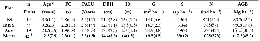
785±57 individuals (ind) ha−1(Table5). For instance, the initial secondary succession (ISS) had, on average, 83 Mg ha−1of AGB and 3.3±1.1 years, the intermediate secondary succession (IntSS) had 99_±18 Mg ha−1_{and 9.2±2.3 years, and the maximum AGB was observed at a 28 years old}

secondary forest plot (AGB = 200.0 Mg ha−1). The average AGB in the ISS was 55% lower than in the Adv. succession, and 20% lower than in the IntSS (Table5). Due to the short time interval of land-use history, the PALU and FC were higher in the ISS and IntSS classes.

Table 5.Mean and standard deviation (in brackets) of structural parameters in secondary forest plots by succession class: ISS—initial secondary succession, IntSS—intermediate secondary succession, and AdvSS—advanced secondary succession. The abbreviations are: FC—frequency of cuts, PALU—period of active land-use, DBH—diameter at the breast height, Ht—total height, G—basal area, S—species density, N—tree density, AGB—aboveground biomass.

Plot n Age * FC PALU DBH Ht G S N AGB

(Plots) (Years) (x) (Years) (cm) (m) (m2_ha−1_{) (sp ha}−1_{) (ind ha}−1_{) (Mg ha}−1₎

ISS 14 3.3(1.1) 2.8(0.5) 3.1(1.7) 11.9(2.8) 13.0(1.4) 14.0(5.6) 29(9) 841(145) 83.2(42.2)

IntSS 9 9.2(2.3) 2.2(1.1) 2.8(1.9) 12.9(1.1) 13.5(0.5) 16.7(2.3) 31(4) 785(57) 99.3(17.8)

Adv 19 20.2(2.6) 1.9(0.9) 1.4(0.5) 17.0(2.3) 15.0(1.1) 24.9(3.8) 49(7) 1274(424) 151.5(30.4)

Mean 42† _{12.2(7.9) 2.3(1.1) 2.3(1.5) 14.4(3.3) 14(1.5) 19.5(6.5) 39(12) 1025(373) 117.2(45.2)}

Note: * Age at the field survey.†_total.

3.2. Growth Models and Accumulation Rates of the Secondary Forests Biophysical Variables

The curves of biophysical variables showed different behavior, indicating distinct accumulation rates. The fitted growth models for mean diameter (DBH), mean forest tree-height (Ht), and species richness (S) did not show a typical sigmoidal shape, but resembled a logarithmic model—inflection point c < 1 (Figure3). As a consequence, the corresponding maximum MAI of these biophysical variables occurs in the first years of the forest life. All model parameters (A, k, and C) were significant forα= 0.05. For instance, mean DBH and mean Ht showed a rapid growth in the SFs of Santaré_m,

reaching half of the PF value in approximately nine and eight years, respectively (Figure3A,B). The MAI of mean DBH was higher than 2 cm year−1in the first five years (Figure3A). The MAI of mean Ht was greater than 1 m year−1during the first 13–14 years (Figure3B), with similar results reported by Neeff and Santos [25].

The basal area (G) was the biophysical parameter that reached the asymptote faster in the SFs, as reported by other authors [12,131]. For instance, SFs recover 90% of G observed in adjacent PF at 19 years age (Figure3C). The maximum MAI of G was estimated at 1.6 m2ha−1year−1and occurred in the fourth year, while [25] observed maximum MAI in the sixth year. Along with the Ht and G, the tree density (N) quickly reached values close to the PFs [25,131]. At the age of 20, SFs have 70% N of the PF (Figure3E). Due to different measurements methodologies regarding minimum DBH measured, we excluded some advanced SF aging plots >20 years from the analysis of tree density.

The S, on the other hand, showed the slowest accumulation rate in the SFs amongst the biophysical variables; the MAI of S was below to 4 sp ha−1year−1in the first 10 years and inferior to 2 sp ha−1 year−1from the age of 25 years (Figure3D). In this S recovery rate, the SFs of the Santarém site would present 72% of the S per hectare observed in the PF at approximately 100 years.

The mean AGB showed intermediate recovering rate. The MAI of AGB occurs at 18th year MAI = 6.6 Mg ha−1year−1(Figure3F). At this growth rate, 50% of the asymptote can be reached at age 25; and 75% at age 44. Considering that approximately 50% of the AGB is organic carbon (C), the potential assimilation of C is greater than 3.7 Mg C ha−1_year−1_{in the Santarém SF up to}

C S

forest hv hh hh hv

C S S

Figure 3.Growth models of mean diameter at breast height (A); mean tree height (B); basal area (C); species density (D); tree density (E); and aboveground biomass (F) in Santarém site by age of secondary forests (continuous black line). Secondary axis represents the relative growth per year (increment). The continuous red line refers to primary forest asymptote. Confidence and prediction intervals are represented in dark and light shaded areas, respectively. Dashed line represents the mean annual increment (MAI).

3.3. Characterization of Secondary Forest with Polarimetric Data

The polarimetric attributes have showed different responses or sensitivity for each biophysical variable, given by the Pearson’s correlation coefficient (Figure4). For instance, the third eigenvalue, associated to the respective eigenvector of the Cloude decomposition (λ3), is related to the magnitude of the cross-polarization signal (HV) and showed the highest correlationρ _≈ 0.6 with DBH, Ht, G, S, and AGB. With the exception of N, these biophysical variables obtained high ρ with the polarimetric attributes related to volumetric scattering, such asλ3, I_C22, the Forest index, and the volumetric scattering mechanisms of Singh, Freeman–Durden, and Yamaguchi decompositions (Figure4). The term I_C22 refers to second element of the diagonal of the covariance matrix [C]3

C22 =2h|SHV|2iand the Forest index refers to the contribution of volumetric and surface backscattering

from forest canopies [124] by (12)

σ0_forest=σ0_hv+σ0_hh.σ

0 hh

σ0_hv (12)

whereσ0_forestis the backscattering from forest canopy,σ0_hvis the volumetric backscattering andσ0_hhis the surface backscattering.

As expected, the AGB, DBH, Ht, G, and S were positively correlated with the volumetric scattering, meaning that SFs areas presented greater volumetric scattering contribution with increasing forest age. However, the N showed no significant correlation with AGB, DBH, and Ht (p-value = 0.19, 0.28, and 0.76, respectively), and were weakly correlated with the SAR attributes. The highest correlation value with N (ρ= 0.30) was the real term off-diagonal of the covariance matrix C23=

√

2_hSHVS∗VVi, although

C S S

T S

S S C S

T S S S

forest hv hh hh hv

T S

Figure 4. Correlation matrix of the highest Pearson coefficients between the biophysical variables of the secondary forests and the polarimetric attributes from ALOS-2 PALSAR-2. Note: Age—secondary forest age; DBH—mean diameter at breast height; Ht—mean tree-height; G—basal area; S—species richness; N—tree density; PALU—period of active land-use; FC—frequency of cuts; l3 and l2—third and second eigenvalue associated to the respective eigenvector of the Cloude decomposition (λ₂ and λ₃); I_C23real—real term off-diagonal of the covariance matrix C23 =

√

2hSHVS∗VVi; TVSM_phi_s—Touzi target phase angle (Φs); Singh_Vol, Freeman_Vol,

and Yamaguchi_Vol—volumetric contribution of the Singh, Freeman–Durden and Yamaguchi decompositions, respectively; TVSM_psi_s1 and TVSM_psi_s3—orientation angle of the first and the third eigenvector of Touzi (ψ_s1andψ_s3), respectively; T23_realC—real term off diagonal of the coherency matrix T23=h(SHH−SVV)S∗HVi; I_C22—second element of the diagonal of the covariance

matrix C22=2h|SHV|2i; TVSM_psi_s—Touzi mean target orientation angle (ψs); T13_real—real term

off-diagonal of the coherency matrix T13 =h(SHH+SVV)S∗HVi; Forest—contribution of volumetric

and surface backscatteringσ0_forest=σ0_hv+σ0_hh.σ0_hh/σ0_hv; T33—third element of the diagonal of the coherency matrix T33=4h|SHV|2i; TVSM_tau_s1—target ellipticity angle of the first eigenvector of

Touzi (τ_s1).

p-value = 0.014, respectively). Interestingly, the polarimetric attributes that were sensitive to the FC were angular decompositions as Touzi target phase angle (Φ_{s), Touzi target ellipticity angle (}τs),

and Touzi target orientation angle (ψs).

The Touzi target phase angle showed a negative and significant correlation with PALU and FC, and also a positive and significant correlation with biophysical variables, being close to zero in high AGB. Touzi [112] describedφ_s=0 as areas with ambiguity between dihedral-trihedral scattering types. SF areas subjected to a longer PALU and higher FC have greater contribution of trihedral scattering type, as shown by the distribution of Touzi target phase angle (φ_s) (Figure5).

Figure 5.Scatter plot between Touzi target phase angle in degrees and period of active land-use in years (PALU). (A) and frequency of cuts in x times (FC); (B) Dashed lines represent the linear regression.

3.4. Modeling AGB

The nonlinear (NL) model showed signal saturation for AGB values close to 150 Mg ha−1using the backscattering coefficient of the cross-polarized channel (σ0HV), as has often been reported in the literature (Figure6A). The fitted NL model has an AIC of 417.1 and low R2_{= 0.28 (Table6) when}

compared to other studies that used similar models R2= 0.44–0.86 [37,132,133]. We argue that this was due to the low amount of data available for the young SFs. In consequence, the mean error in the initial secondary succession (ISS) was higher than in the IntSS and advanced succession (Table6). The RMSE from NL model represented about 12% of the mean value of the AGB (RMSE = 39.7_±6.8 Mg ha−1_,

Table6). The NL model had a bias of the estimateµ_bias= 0.26±38.3 Mg ha−1and did not different from zero by thet-test (Figure7I), besides of the tendency of overestimating the AGB > 150 Mg·ha−1 (Figure7A).

The young SFs have higher MAI of AGB and higher sensitivity to SAR microwave wavelength, which, in turn, has higher variability response of the radar signal than older SFs [25,39]. The standardized residues, otherwise, were heteroscedastic, rejecting the hypothesis of homoscedasticity of the residuals at the levelα= 0.05 (BP: 4.8;p-value < 0.05, Figure6B).

Due to the great number of polarimetric attributes tested (total of 125, Table4and AppendixA

Table A1) the correlation filter selection (CFS) was used to choose the best subset for applying MLR. According to the CFS selection and leave-one-out criteria, only nine polarimetric attributes were selected with the highest importance value and ten models by the Akaike criteria ∆_{AIC < 2}

(Supplementary Materials, Figure S2).

The attributes that presented the highest relative importance in the MLR models were: the real term T12 between the channels (HH + VV) and (HH − VV) of the Barnes–Holm decomposition,

the target ellipticity angle (τ) of the Neumann decomposition (Neumann_τ), and the target ellipticity angle (τ) of the third eigenvector of Touzi decomposition (TVSM_tau_s3) (Supplementary Materials, Figure S2).

The attributes of the Touzi decomposition as the Touzi target magnitude and the phase are commonly reported to present important information for modeling AGB in the tropics [37,79,83]. Bispo et al. [37] observed a high correlation between the AGB and the target ellipticity angle, but only for the first Touzi eigenvector (τ_s1) and did not for the third as described here (τ_s3).

Among the 10 models pre-selected by the∆_{AIC < 2 the best model presented AIC = 407.42 with}

seven prediction polarimetric attributes, against AIC = 408.13 and AIC = 408.14 for the second and third best models with six and five attributes, respectively. However, the first and third models presented high variance inflation factor (VIF) values for theλ₃and T23_imagB attributes, which both also have high correlation with AGB, indicating multicollinearity problems. So, the best MLR model was the second Equation (13)

AGBMgha−1= −1151.1+516.6(Neumann_τ) +0.96(τ_s3) +2809.1 T23imag +592.91(SEPnorm) +319.52(SEnorm) +2306.73(T12realB)

(13)

The selected model (Equation (13)) was able to explain slightly more than 50% of the AGB variability in the Santarém’s SF (R2adj.= 0.51), whose parameters were significant at theα= 0.05 level,

except for theτ_s3 and the imaginary component T23of the matrix [T] that were significant at the

α= 0.1 level.

Interestingly, the prediction polarimetric attributes of the MLR model did not have the highest correlation with the AGB. For instance, the target ellipticity angle of Neumann decomposition (Neumann_τ) had highest and significant correlation with the G (p-value < 0.001); and the normalized Shannon Entropy (SEnorm) with the mean DBH (p-value = 0.001). These attributes also showed

a significant correlation with the AGB, Ht, and S at theα= 0.05 level. Theτ_s3 presented a higher correlation with the AGB, although it was not significant (p-value > 0.05). The T12_realB term of the Barnes–Holm decomposition and the T23imag have a negative correlation with the PALU (p-value = 0.18 andp-value = 0.42, respectively). The contribution of the degree of depolarization of the normalized Shannon entropy (SEPnorm), in turn, showed a higher and not significant correlation

with the G. The regression residuals presented a normal distribution (p-value = 0.64), without the presence of possible outliers (Supplementary Materials, Figure S3), and we did not reject the hypothesis of homoscedasticity of the residuals at the levelα= 0.05 by the Breusch–Pagan test (BP: 3.46,p-value = 0.063).

forests, which culminates in high variations of the observed AGB. These differences on structural parameters will gradually disappear with the aging of the forest. After the age 20, the forest AGB is underestimated by the models (Figure7C,D). However, this underestimation is more evident with the NL model (Figure7C) due to saturation signal of the backscattering signal at high forest AGB.

Table 6. Model’s performance evaluation. NL—nonlinear, MLR—multiple linear regression, RMSE—Root mean square error, ISS—initial secondary succession, IntSS—intermediate secondary succession, AdvSS—advanced secondary succession, PALU—period of active land-use.

AIC R2 Validation

RMSE (Mg ha−1₎

RMSE ISS

RMSE IntSS

RMSE Adv

RMSE PALU 1–2 years

RMSE PALU 3–4 years

RMSE PALU >4 years

Bias (Mg ha−1₎

NL 417.1 0.28 39.7 50.9 34.6 38.2 45.4 33.2 31.3 0.3

MLR 408.1 0.37 38.7 52.6 37.7 33.8 37.6 43.6 21.8 2.1

Considering the PALU, the errors were consistently higher in the low intensity SFs areas, regardless of age (Table6, Figure7E,F). The possible reason is due to areas of light-use showed greater species compositions and richness that presented greater variation of their structural parameters that are sensitive to SAR parameters. On the other hand, there is no trend in the bias error of the AGB models regarding the cut frequency (Figure7G,H). The errors are between the±100 Mg ha−1 regardless of the number of the clear cuts (Figure7G,H).

The RMSE of the MLR after cross-validation was RMSE = 38.7± 9.8 Mg ha−1 and the AGB prediction showed no clear signal saturation when multiple polarimetric attributes were combined (Figure7B). However, prediction errors were higher in low AGB values because of multiple interactions between attributes resulted in spurious values resulting from low sampling at AGB about 20–70 Mg ha−1. The mean bias error of MLR was higher than in the NL modelµ_bias= 2.1±37.9 Mg ha−1(Figure7D) and it was not different from zero by thet-test (p-value = 0.1).

Figure 7. Bootstrapped cross-validation results for AGB estimation in the secondary forests using non-linear (A,C,E,G,I) and multiple linear regression model (B,D,F,H,J). (A,B) Linear regression between reference AGB (x-axis) and predicted AGB (y-axis). The solid line represents the perfect 1:1 fit and the dotted line the adjustment after cross validation; (C,D) Bias of prediction by secondary forest age; (E,F) Bias of prediction by period of active land use (PALU) before abandonment; (G,H) Bias of prediction by frequency of cuts (FC); (I,J) Probability density function and histogram of bias of prediction AGB.

Figure 8.(A) Map of above-ground biomass (AGB, Mg ha−1) in the secondary forests of Santarém with the non-linear (NL) model, and (B) with multiple linear regression (MLR) model. The background image is Landsat 5 TM false color composite 5-4-3 from 25 July 2015.

4. Discussion

4.1. Growth Models for Biophysical Variables

By analyzing the empirical models we showed that biophysical variables had different accumulation rates. While DBH, Ht, G, and N could quickly recover during the regrowth of SFs, the AGB and S took a much longer time to recover the PFs values. So, the classification of the SF in the ISS, IntSS, and AdvSS should not be only based on structural parameters or species richness and composition [12]. Pioneer species comprise 33% of the S and almost 40% of the N in the Santarém study site [63,64]. The most common species wereGuatteria poeppigianaMart. andCasearia grandiflora

Cambess, a pioneer species and early secondary species, respectively, which are virtually absent in the PFs and have a lifespan superior than 50 years [81]. Such findings have implications for modeling tree growth, as reported by Cassol et al. [63], who observed a higher initial MAI of the Ht in the secondary species in relation to pioneer species at the same study site.

Our results demonstrated the patterns of growth for different SF biophysical variables in the Santarém study site. Although the graphs showed the growth curves up to a 40-year interval, the input data included SFs younger than 30 years-old. This was the reason why the growth models tested could not be fitted without the asymptote being fixed—second model assumptions [25]. The age distribution of plots (up to 28 years) is quite narrow as the most pioneer species ages (48–162 years), so this approach might be less useful at more advanced stages of secondary succession [2,81].

an older forest. For instance, Lebrija-Trejos [131] observed that N, S, and crown cover may exceed the values of mature forest in less than 40 years in a dry tropical deciduous forest, southern Mexico. Here, the fast accumulation of G was observed, overtaking the primary forest in some plots at age 20. So, the asymptote should not have been the same at this high variability sample plots, since it depends of other sources of variability as water and soil nutrient availability [89]. However, the small number of sampling plots limited our growth analysis at different environment conditions or land-use history.

Our results of SFs growth did not match observations made by Neeff and Santos [25], who found out the asymptote in the 40–50 years for AGB of young SFs in the Santarém site. However, they used power model for modeling AGB growth and fixed the maximum AGB values to 192.8 Mg ha−1for the mature forest. Other authors depicted similar accumulation of biomass in young SF up to 100 Mg ha−1 at less than 15 years [2]. Houghton et al. [16] considered a superior AGB accumulation in their model at age 25, with almost 70% of AGB from PFs. The Houghton’s model was obtained by the product of the growth rate estimated by Brown and Lugo [2] MAI = 11 Mg ha−1year−1for SF < 10 years in the entire Brazilian Amazon, regardless of the land-use history [2]. Our value of MAI is almost 2.5 times higher than the 1.5 Mg C ha−1year−1estimated by Houghton et al. [16] for SFs with AGB < 100 Mg ha−1 used in the model of annual carbon flux from regeneration areas in the Brazilian Amazon. We argue that the absence of emergent slow growth species, which have the largest contribution to AGB [60], as a possible cause for reducing the accumulation of AGB in our study at age 25.

These growth models are not only applicable for estimating biophysical variables of the SFs using ALOS-2 PALSAR-2 data, but also for carbon budget estimation and ecological application. The chronosequences of SFs were obtained in areas that suffered distinct land-use intensities and despite neglecting them in growth models it is rely on assumptions relating to the ecological process of the forest growth. The modeling of SF growth by land-use history was explored by Wandelli and Fearnside [26] in the central Amazonia. They found a 38% lower AGB accumulation at age 6 in the areas following pasture than that following slash-and-burn agriculture. These findings have implications for the estimation of carbon throughout the Amazon when the historic of land-use is not considered, because the uncertainties in the mapping of AGB increase.

The results of growth models indicate that the SF monitoring in the tropics should cover a broader range of ages, specifically including SFs older than 100 years. The widening of the age spectrum would allow an increase in accuracy of growth models due to a better characterization of the underlying sources of variation, such as the intensity of previous use, soil characteristics, and water availability, among others. These long-term surveys could be useful to confirm the hypothesis of the different degrees of SF resilience across the Amazon Basin [135,136].

4.2. Polarimetric Data for SF Characterization

The polarimetric attributes extracted from the ALOS-2 PALSAR-2 data showed different sensitivity with the biophysical variables. In general, the volumetric scattering from canopies was most correlated with the structural parameters (DBH, Ht, G, S, and AGB), whilst angular decomposition were most correlated with land-use history. These differences in the polarimetric attributes responses of PALU and FC can be attributed by the structural differences in the regrowth pathways. The high intensity of past-use reduces the complexity of the secondary forest by reducing not only the AGB, but also the species richness and composition [18,36]. For instance, the increment of the AGB in areas previously burned 4–5 times can be 50% less than in the areas abandoned right after clear-cut [35]. Uhl et al. [18] reported a strong reduction in biomass accumulation at eight years of the SF in the Central Amazon. The AGB was 60–87 Mg ha−1after 1 year of grazing, 28 Mg ha−1with 6 years of grazing and only 0.16 Mg ha−1with 11 years of grazing. This slow increment related to past land-use was significant up to 18-years-old, but disappear at AdvSS [36]. Such differences on structural parameters of the SFs could highlight the divergences among polarimetric attributes by land-use history and biophysical variables.

the initial secondary succession may reduce the power of the polarimetric data to detect the complex structure and the rapid AGB accumulation of the SFs. Another limitation for characterizing the SFs by land-use history was the differences in age between them, in which, on average, the light land-use of SFs were older than high use of SF, due to the short interval of Landsat time-series classification.

The high importance of the angular polarimetric attributes of the Touzi and the Cloude and Pottier decompositions have been reported as a great predictor for modeling and mapping forest AGB [37,45,46], although the subjacent process that causes the signal response are not fully understood. A controlled experiment is needed in an effort to better understand the role of biophysical variables such as tree density, and not just forest AGB, in the response of the polarimetric attributes, in particular the angular attributes.

4.3. Regression Models

Our results showed good performance of the regression models varying from R2 _{= 0.38 for}

the non-linear model to R2 = 0.51 for the MLR model. The regression models presented weaker performance of the NL and MLR models using L-band data in the Brazilian Amazon SFs, whose R2 found was R2> 0.67 [45,132,133]. Kuplich et al. [133] generated a AGB forest map for two different regions of the Brazilian Amazon (Manaus and Santaré_{m) and presented better performance when SAR}

texture was included in the model, while Foody et al. [132] attained good model performance when the forest plots were divided in toCecropiasp. and nonCecropia-dominated forest.

In the MLR, multiple scattering mechanisms and other parameters of SAR decomposition as the phase and orientation angles in one resolution cell can be used as prediction variables instead of only using the backscattering coefficient. However, MLR can have some limitations, namely, in terms of parameter interpretation and over fitting (many prediction variables). In the selected MLR model (Equation (13)) it was observed the importance of polarimetric attributes not commonly used for AGB estimation as the off-diagonal terms of the coherency and covariance matrices. The hypothesis that forested areas show reflection symmetry can be denied by the increasing value of the T23_imag and T12_realB terms, since according to Lee and Pottier [137] the terms off-diagonal are null if they satisfy the condition of reflection symmetry (monostatic case). This observation motivated us to apply unusual terms as angular responses from decompositions as well as the off-diagonal element of the [T] and [C] as prediction variables, despite the fact that their physical relationship with forest targets is not fully understood.

The importance off-diagonal terms of the [C] and [T] has been neglected from analysis in the literature by believe they were null under reflection symmetry assumption. Instead of being highly correlated to AGB given its relative importance in the MLR model, they were correlated to other biophysical variables such as the N, G, and average DBH, which in turn are related to the previous land-use. Furthermore, recent polarimetric decompositions approaches such as Shannon entropy and Neumann also presented good relationships with AGB and can be useful for other forest applications [108 < 106,118 < 117]. The use of terms off-diagonal of the [C] and [T] for forest studies with different structures, densities, and types is still a field to be developed.

4.4. Uncertainty Report

Several sources of uncertainty could be identified which are mainly originated by the propagation of errors from the field data to remote sensing analysis [138]. These errors included inherent inventory errors, the choice of the hypsometric equation for height estimation, the allometric equation for the AGB estimation, and the expansion errors of individual trees for the plot analysis. In addition, the errors related to the growth modeling and from the land-use history, the errors of the geometric co-registration and orthorectification, the inherent errors of the sensor instrument and, finally, the errors from regression models.

defined as the sampling error to expand the sum of individuals in the plot to the hectare described in Cassol [65]. The errors of AGB growth models were RMSE = 5.4% and the ones from the history of use were on average 17% [28]. Inherent sensor instrument errors include speckle noise, calibration errors, topographic effects, and variability sources as moisture content, but they were not computed here. The value modeled by the sum of these components calculated by Ahmed et al. [139] was

σ◦= 0.025 dB, that is, less than 2% of the mean backscatter coefficient of the SF. Co-registration errors were not computed, but were smoothed due to the use of the mean of the attributes in each plot. The errors from MLR model were RMSE = 33%.

The error propagation was not modeled, but a good approximation can be made computing the mean errors, considering that they are independent and not correlated with each other [138]. In such a case, the mean error of AGB estimation was 18.6% considering all the mentioned sources of uncertainty. It is noted that the errors related to the choice of the allometric equation for the individual biomass estimation and to the expansion of the individual tree analysis for the plot analysis represent more than 50% of the total errors in Santaré_{m site. It was due to the allometric equations}

for AGB estimation are, in most cases, generated from individuals of primary forests, resulting in an overestimation of the secondary forests AGB. The use of specific gravity may help to overcome this issue by reducing the mean specific gravity of the sum of the individuals in one hectare. However, the best option is the use of the species-specific allometric equations when available. The smallest errors come from SAR data and processing, as well as from the regression models, which were less than 20% of the average total errors.

5. Conclusions

The main goal of this research was to retrieve secondary forest (SF) aboveground biomass (AGB) at the Santarém site using the polarimetric ALOS-2 PALSAR-2 data. The Chapman-Richards (CR) models were used to update the biophysical variables to PALSAR-2 acquisition date time. According to these models, the mean diameter (DBH), mean tree-height (Ht), and basal area (G) presented highest increment amongst the biophysical variables, reaching half of asymptote in less than 15 years. The AGB and the species richness (S) may reach half of asymptote after 25 years, and 90% of asymptote beyond 100 years. Such finds have implications to biodiversity conservation and carbon sink purposes, since SFs are often recleared earlier.

The angular polarimetric attributes, as those from the Touzi decomposition, were more related to the land-use history, whilst the contribution of volumetric scattering was significantly correlated with the biophysical variables (forest structure). The period of active land-use and frequency of clear cuts showedρ= 0.37 (p-value = 0.0175) andρ= 0.38 (p-value = 0.014) with the Touzi phase module angle (Φ_{s), respectively. The biophysical variables, such as mean DBH, mean Ht, G, S, and AGB}

were strongly correlated with the Cloude third eigenvalue (λ₃) (p-value < 0.001). The influence of SF historical use on angular decompositions is an open field to be explored in future research.

The reflection symmetric condition under forest environments was denied, given by the relative importance of the terms off-diagonal from covariance and correlation matrix in the MLR model, which violates the main polarimetric decomposition assumptions. Thus, the authors believe that the generation of new polarimetric decompositions directly from the T4 matrix (bistatic case) is a field to be explored in the future, incorporating the asymmetry nature of these targets in the polarimetric response.

Supplementary Materials:The following are available online athttps://www.mdpi.com/2072-4292/11/1/59/s1. Author Contributions:H.L.G.C. developed the research, conceived, designed the experiments, and also analyzed the data and wrote the article. Y.E.S. and E.C.M. supervised all stages of the research as advisors and also comments. J.M.d.B.C. provided the ALOS-2 data, contributed for methodological and discussion analysis, L.E.O.e.C.d.A. contributed to editing, revision, and discussion of the paper. C.V.d.J.S. provided field sample data of young secondary forest and helped with revision manuscript. S.Q. contributed to editing and discussion.

Funding: The H.L.G.C. was founded by FAPESP (2018/14423-4). J.M.d.B.C. work was supported by the Natural Environment Research Council (Agreement PR140015 between NERC and the National Centre for Earth Observation). The L.E.O.e.C.d.A. was founded by CNPq (Grant 305054/2016-3).

Acknowledgments: The authors are grateful to the Coordenação de Aperfeiçoamento de Pessoal de Nível Superior (CAPES), the Conselho Nacional de Desenvolvimento Cientí_{fico e Tecnol}ó_{gico (CNPq), the Instituto}

Nacional de Pesquisas Espaciais (INPE), the REGROWTH-BR Project, and the G-FOI project. We thanks to JAXA and the Kyoto & Carbon Initiative for providing ALOS-2 PALSAR-2 data. Thanks are also given to the botanical assistance Chico, Graveto, and Letícia and the Large-Scale Biosphere–Atmosphere Experiment in Amazonia (LBA-Santarém Office) for the logistic support during the field surveys.

Conflicts of Interest:The authors declare no conflict of interest. The founding sponsors had no role in the design of the study; in the collection, analyses, or interpretation of data; in the writing of the manuscript, or in the decision to publish the results.

Appendix A

Table A1.List of abbreviations, acronyms, and variables.

AdvSS Advanced Secondary Succession

AIC Akaike information criterion ALOS-2 Advanced Land Observation Satellite-2 C, [C], [C]₃ Covariance 3_×3 matrix

CDB Convention on Biological Diversity CF Calibration coefficient factor (dB) CFS Correlation-based feature selection DEM Digital elevation model

FC Frequency of cuts (_×times) FLONA National forest, in Portuguese

FR Faraday rotation (Ω) FRA Forest resources assessment

I Phase image

IntSS Intermediate secondary succession ISS Initial secondary succession LULUCF Land use, land-use change, and forestry

MAI Mean annual increment MCSM Multiple-component scattering model

MLR Multiple linear regression

NL Non-linear

OLS Ordinary least squares

PALSAR-2 Phased Array L-band Synthetic Aperture Radar-2 PALU Period of active land use (years)

PF Primary forest

PRODES Program for Monitoring Deforestation of the Amazon by Satellite Q Complex image phase quadrature