This is a repository copy of
Are Short Proofs Narrow? QBF Resolution is not so Simple
.
White Rose Research Online URL for this paper:
http://eprints.whiterose.ac.uk/123219/
Version: Accepted Version
Article:
Beyersdorff, O orcid.org/0000-0002-2870-1648, Chew, L, Mahajan, M et al. (1 more
author) (2018) Are Short Proofs Narrow? QBF Resolution is not so Simple. ACM
Transactions on Computational Logic, 19 (1). 1. ISSN 1529-3785
https://doi.org/10.1145/3157053
© 2017, the authors. This is the author's version of the work. It is posted here by
permission of ACM for your personal use. Not for redistribution. The definitive version was
published in ACM Transactions on Computational Logic (TOCL), 19 (1), January 2018,
http://doi.acm.org/0.1145/3157053. Uploaded in accordance with the publisher's
self-archiving policy.
Reuse
Unless indicated otherwise, fulltext items are protected by copyright with all rights reserved. The copyright exception in section 29 of the Copyright, Designs and Patents Act 1988 allows the making of a single copy solely for the purpose of non-commercial research or private study within the limits of fair dealing. The publisher or other rights-holder may allow further reproduction and re-use of this version - refer to the White Rose Research Online record for this item. Where records identify the publisher as the copyright holder, users can verify any specific terms of use on the publisher’s website.
Takedown
If you consider content in White Rose Research Online to be in breach of UK law, please notify us by
Are Short Proofs Narrow? QBF Resolution is
not
so Simple
OLAF BEYERSDORFF, School of Computing, University of Leeds, United Kingdom LEROY CHEW, School of Computing, University of Leeds, United Kingdom
MEENA MAHAJAN, The Institute of Mathematical Sciences (HBNI), Chennai, India ANIL SHUKLA, The Institute of Mathematical Sciences (HBNI), Chennai, India
The groundbreaking paper ‘Short proofs are narrow – resolution made simple’ by Ben-Sasson and Wigderson (J. ACM 2001) introduces what is today arguablythemain technique to obtain resolution lower bounds: to show a lower bound for the width of proofs. Another important measure for resolution is space, and in their fundamental work, Atserias and Dalmau (J. Comput. Syst. Sci. 2008) show that lower bounds for space again can be obtained via lower bounds for width.
In this paper we assess whether similar techniques are effective for resolution calculi for quantified Boolean formulas (QBF). There are a number of different QBF resolution calculi like Q-resolution (the clas-sical extension of propositional resolution to QBF) and the more recent calculiAExp+ResandIR-calc. For these systems a mixed picture emerges. Our main results show that both the relations between size and width as well as between space and width drasticallyfailin Q-resolution, even in its weaker tree-like ver-sion. On the other hand, we obtain positive results for the expansion-based resolution systemsAExp+Res
andIR-calc, however only in the weak tree-like models.
Technically, our negative results rely on showing width lower bounds together with simultaneous up-per bounds for size and space. For our positive results we exhibit space and width-preserving simulations between QBF resolution calculi.
Categories and Subject Descriptors: F.2.2 [Analysis of Algorithms and Problem Complexity]: Nonnu-merical Algorithms and Problems—Complexity of proof procedures
General Terms: Algorithms, Theory
Additional Key Words and Phrases: Proof complexity, QBF, resolution, lower bound techniques, simulations
ACM Reference Format:
Olaf Beyersdorff, Leroy Chew, Meena Mahajan, and Anil Shukla, 2016. Are short proofs narrow? QBF reso-lution isnotsimple.ACM Trans. Comput. LogicV, N, Article A (January YYYY), 27 pages.
DOI:http://dx.doi.org/10.1145/0000000.0000000
1. INTRODUCTION
The main objective inproof complexityis to obtain precise bounds on the size of proofs in various formal systems; and this objective is closely linked to and motivated by foundational questions in computational complexity (Cook’s program), first-order logic (separating theories of bounded arithmetic), and SAT solving. In particular, proposi-tional resolution is one of the best studied and most important proposiproposi-tional proof sys-tems, as it forms the backbone of modern SAT solvers based on conflict-driven clause learning (CDCL) [Marques-Silva et al. 2009]. Complexity lower bounds for resolution
This work was supported by the EU Marie Curie IRSES grant CORCON, grant no. 48138 from the John Templeton Foundation, EPSRC grant EP/L024233/1, and a Doctoral Training Grant from EPSRC (2nd au-thor).
A preliminary version of this article appeared in the proceedings of the conference STACS’16 [Beyersdorff et al. 2016].
Permission to make digital or hard copies of all or part of this work for personal or classroom use is granted without fee provided that copies are not made or distributed for profit or commercial advantage and that copies bear this notice and the full citation on the first page. Copyrights for components of this work owned by others than ACM must be honored. Abstracting with credit is permitted. To copy otherwise, or repub-lish, to post on servers or to redistribute to lists, requires prior specific permission and/or a fee. Request permissions from [email protected].
c
YYYY ACM. 1529-3785/YYYY/01-ARTA $15.00
proofs directly translate into lower bounds on the performance of SAT solvers [Sabhar-wal 2005; Buss 2012].
What is arguably even more important than showing these actual bounds is to de-velop general techniques that can be applied to obtain lower bounds for important proof systems. A number of ingenious techniques have been designed to show lower bounds for the size of resolution proofs, among them feasible interpolation [Kraj´ıˇcek 1997], which applies to many further systems. In their pioneering paper Ben-Sasson and Wigderson [2001] showed that resolution size lower bounds can be elegantly ob-tained by showing lower bounds to thewidth of resolution proofs. Here, the size of a proof denotes the number of its clauses, and the width of a proof is the length of the biggest clause in it. Indeed, the discovery of this relation between width and size of resolution proofs was a milestone in our understanding of resolution, and today many if not most lower bounds for resolution are obtained via the size-width technique.
Another important measure for resolution isspace[Esteban and Tor ´an 2001], as it corresponds to memory requirements of solvers in the same way as resolution size re-lates to their running time. Informally, the space complexity for refuting a formula in resolution is the minimum number of clauses that must be kept in memory simulta-neously to refute the formula. In their fundamental work Atserias and Dalmau [2008] demonstrated that also space is tightly related to width. Indeed, showing lower bounds for width serves again as the primary method to obtain space lower bounds. Since these discoveries the relations between resolution size, width, and space have been subject to intense research (cf. [Beyersdorff and Kullmann 2014]), and in particular sharp trade-off results between the measures have been obtained (cf. e.g. [Beame et al. 2012; Ben-Sasson and Nordstr¨om 2011; Nordstr¨om 2013]).
In this paper we initiate the study of width and space in resolution calculi for quan-tified Boolean formulas (QBF) and address the question whether similar relations be-tween size, width and space as for classical resolution hold for QBF calculi. Quantified Boolean formulas are propositional formulas where each variable is quantified with either an existential or a universal quantifier. Before explaining our results we sketch recent developments in QBF proof complexity.
QBF proof complexity is a relatively young field studying proof systems for quan-tified Boolean logic. As in the propositional case, one of the main motivations for the field comes via its intimate connection to solving. Although QBF solving is at an earlier state than SAT solving, it offers great potential. Due to itsPSPACEcompleteness, QBF
allows for more succinct encodings and therefore QBF solving applies to further fields such as formal verification or planning [Rintanen 2007; Benedetti and Mangassarian 2008; Egly et al. 2017]. Each successful run of a solver on an unsatisfiable instance can be interpreted as a proof of unsatisfiability; and this connection turns proof com-plexity into the main theoretical tool to understand the performance of solving. As in SAT, many QBF solvers implement decision procedures that have resolution (and its variants) as their underlying proof system.
expansion-based solving were recently developed in the form ofAExp+Res[Janota and Marques-Silva 2015], and the strongerIR-calcandIRM-calc[Beyersdorff et al. 2014].
In this paper we concentrate on the three QBF resolution systemsQ-Res,AExp+Res, andIR-calc. This choice is motivated by the fact thatQ-Res andAExp+Resform the base systems for CDCL and expansion-based solving, respectively, andIR-calcunifies both approaches in a natural way, as it simulates bothQ-ResandAExp+Res [Beyers-dorff et al. 2014]. Recent findings show that CDCL and expansion are indeed orthogo-nal paradigms asQ-ResandAExp+Resare incomparable with respect to simulations [Beyersdorff et al. 2015].
Understanding which lower bound techniques are effective in QBF proof complexity is of paramount importance for progress in the field. By Beyersdorff et al. [2017] it was shown that the feasible interpolation technique of Kraj´ıˇcek [1997], transferring (monotone) circuit size lower bounds to proof size lower bounds, applies to all QBF resolution systems. Another successful transfer of a classical technique was obtained by Beyersdorff et al. [2017] for a game-theoretic characterisation of proof size in tree-likeQ-Res.
Our contributions
The central question we address here is whetherlower bound techniques via width, which have revolutionised classical proof complexity, are also effective for QBF resolu-tion systems.
Though space and width have not been considered in QBF before, these notions straightforwardly apply to QBF resolution systems. However, due to the∀-reduction rule inQ-Resallowing removal of universal variables from clauses (under certain side conditions), it is relatively easy to enforce that universal literals accumulate in clauses of Q-Res proofs, thus always leading to large width, irrespective of size and space requirements (Lemma 3.6). This prompts us to considerexistential width— counting only existential literals — as an appropriate width measure in QBF. This definition aligns both with Q-Res, which only resolves on existential variables, as well as with A
Exp+Res and IR-calc, which like all expansion systems only operate on existential literals.
1. Negative results. Our main results show that the size-width relation of Ben-Sasson and Wigderson [2001] as well as the space-width relation of Atserias and Dal-mau [2008] dramaticallyfailforQ-Resin the sense that there exist formulas requiring maximal (linear) width, but allowing for proofs of minimal (polynomial) size and min-imal (constant) space. This even holds when considering the tighter existential width. We first notice that the proof establishing the size-width result of Ben-Sasson and Wigderson [2001] almost fully goes through, except for some very inconspicuous step that fails in QBF (Proposition 4.1). But not only the technique fails: we prove that Tseitin transformations1 of formulas expressing a natural completion principle2 of
Janota and Marques-Silva [2015] have small size and space, but require large exis-tential width in tree-like Q-Res(Theorem 4.2), thus refuting the size-width relation for tree-likeQ-Resas well as the space-width relation for general dag-likeQ-Res.
As the number of variables in the formulas for the completion principle is quadratic in their refutation width, these formulas do not rule out size-width relations in general Q-Res. However, we show that a different set of formulas, hard for tree-like Q-Res [Janota and Marques-Silva 2015], provide counterexamples for size-width relations in fullQ-Res(Theorem 4.9).
1
Tseitin transformations are a standard technique to transform arbitrary propositional formulas into 3-CNFs by using additional variables. Here we use that fact that they produce constant-width formulas.
2
Technically, our main contributions are width lower bounds for the above formulas, which we show by careful counting arguments. We complement these results by exis-tential width lower bounds for parity-formulas of Beyersdorff et al. [2015], providing an optimal width separation betweenQ-ResandAExp+Res(Theorem 5.6).
2. Positive results and width-space-preserving simulations.Though the neg-ative picture above prevails, we prove some positive results for size-width-space rela-tions for tree-like versions of the expansion resolution systemsAExp+ResandIR-calc. Proofs inAExp+Rescan be decomposed into two clearly separated parts: an expansion phase followed by a classical resolution phase. This makes it easy to transfer almost the full spectrum of the classical relations toAExp+Res(Theorem 6.1).
To lift these results toIR-calc(Theorem 6.2), we show a series of careful space and width-preserving simulations between tree-likeQ-Res,AExp+Res, andIR-calc. In par-ticular, we show the surprising result that tree-likeAExp+Resand tree-likeIR-calcare polynomially equivalent (Lemma 5.3), thus providing a rare example of two proof sys-tems that coincide in the tree-like, but are separated in the dag-like model [Beyersdorff et al. 2015]. The only other such example that we are aware of is regular resolution vs. full resolution (although this is perhaps slightly less natural as regular resolution is just a sub-system of resolution). In addition, our simulations provide a simpler proof for the simulation of tree-like Q-Res by AExp+Res(Corollary 5.5), shown by Janota and Marques-Silva [2015] via a substantially more involved argument.
Our last positive result is a size-space relation in tree-like Q-Res (Theorem 6.2), which we show by a pebbling game analogous to the classical relation by Esteban and Tor ´an [2001]. Not surprisingly, this only positive result forQ-Resavoids any reference to the notion of width.
We highlight that throughout this article we deal with QBF resolution systems that can only resolve on existential variables, a restriction that is crucial for some of our results. This condition holds for the base systemsQ-ResandAExp+Resas well as the stronger systemIR-calc. To clarify the size-width relation for QBF resolution systems likeQU-Resof Van Gelder [2012], which allow resolution steps on universal variables, remains an open problem (cf. also the discussion in Section 7).
As the bottom line we can say that QBF proof complexity is not just a replication of classical proof complexity: it shows quite different and interesting effects as we demonstrate here. Especially for lower bounds it requires new ideas and techniques. We remark that in this direction, a new and ‘genuine QBF technique’ based on strategy extraction was recently developed, showing lower bounds forQ-Res[Beyersdorff et al. 2015] and indeed much stronger systems [Beyersdorff et al. 2016; Beyersdorff and Pich 2016].
Organisation of the paper
2. NOTATIONS AND PRELIMINARIES
We assume familiarity with basic notions from logic, including propositional and quan-tified Boolean logic. We just review those concepts here that are subsequently needed, also setting the notation for later sections. For background information and a rigorous syntactic and semantic definition of the logics we refer to the monograph of Kleine B ¨uning and Lettmann [1999].
Quantified Boolean Formulas.A literal is a Boolean variable or its negation. We say a literalxis complementary to the literal¬xand vice versa. Aclauseis a disjunction
(∨)of literals and atermis a conjunction(∧)of literals. The empty clause is denoted by 2, and is semantically equivalent to false. A propositional formula inconjunctive normal form(CNF) is a conjunction of clauses. For a literall =xorl =¬x, we write
var(l)forxand extend this notation to the setvar(C)of variables of a clauseC. A partial assignmentαfor a set of variablesX is a partial functionα:X → {0,1}. We say that a variable xis assigned a value inαifxis in the domain ofα, denoted
x∈dom(α). We denote an assignmentb ∈ {0,1}to a single variablexby the notation x/b. A partial assignment α is specified as a set of such singleton assignments, eg
{x1/0, x3/1}.
Letαbe any partial assignment. For a clauseC, we writeC|αfor the clause obtained
by applying the partial assignmentαto C. That is, we remove literals falisfied byα
from C, and further, if some literal ofC is true under α, thenCα is the tautological
clause 1. For example, applying α = {x1/0} to the clauseC = (x1∨x2∨x3) yields C|α = (x2∨x3), and applying α′ ={x1/1} to the same clause givesC|α′ = 1. We say
that a partial assignment α satisfies a clause C if C|α = 1, and it satisfies a CNF
formulaF if it satisfies each of the clauses ofF.
LetA, Bbe propositional formulas. We say thatA|=Bholds, if any (partial) assign-ment which satisfiesAalso satisfiesB. LetF be a CNF formula, andxbe a variable inF. ThenF|x/1is a CNF formula obtained fromF by removing all clauses containing
the literalx, and removing all occurrences of the literal¬x. The CNF formulaF|x/0is
similarly defined.
We consider quantified Boolean Formulas (QBFs) inclosed prenex formwith a CNF matrix3, i.e., we consider the form Q
1x1· · · Qnxn.φ where each Qi is either ∃ or ∀,
andφis a quantifier-free CNF formula in the variablesx1, . . . , xn. Such formulas are
succinctly denoted asQφ, whereφis called thematrix, andQis itsquantifier prefix. Given a variable y, either existentially quantified or universally quantified inQφ, the quantification levelof y inQφ, lv(y), is the number of alternations of quantifiers
y has on its left in the quantifier prefix ofQφ. Given a variabley, we will sometimes refer to the variables with quantification level lower thanlv(y)as variablesleftof y; analogously the variables with quantification lever higher thanlv(y)will berightofy. The semantics of QBFs can be defined via a 2-player game between a universal and an existential player (cf. e.g. [Arora and Barak 2009]) or via an inductive truth definition, using that ∀x.F is equivalent to F|x/0∧F|x/1 and ∃x.F to F|x/0 ∨F|x/1
(cf. [Kleine B ¨uning and Lettmann 1999]).
Resolution Calculi
Resolution (Res), introduced by Blake [1937] and Robinson [1965], is a refutational proof system for formulas in CNF. The lines in the Res proofs are clauses. Given a CNF formulaF,Rescan infer new clauses according to the resolution inference rule:
3Any QBF can be efficiently (in polynomial time) converted to an equivalent QBF in this form. See for
C∨x D∨ ¬x (Res).
C∨D
HereC, Ddenote clauses andxis a variable being resolved, called thepivotvariable. The clauses C∨x and D ∨ ¬x are referred to as the hypotheses and C ∨D is the conclusion (resolvent) of the resolution rule.
Let F be an unsatisfiable CNF formula. A resolution proof (refutation) π of F is a sequence of clauses D1, . . . , Dl, where Dl = 2, and each clause in the sequence is
either from F or is derived from some previous clauses of the sequence via the above resolution rule.
We say that a directed acyclic graph (dag) G = (V, E)represents the refutation π
ifV = {D1, . . . , Dl}, the source nodes are the clauses from F, internal nodes are the
derived clauses, and the empty nodeDlis the unique sink. Furthermore, edges inGare
from the hypotheses to the conclusion for each resolution step. That is, each derived clauseDihas incoming edges fromDjandDkwhere the indicesj, kare less thani, and
Diis the resolvent ofDj andDk. (Since a clause could be derived from more than one
set of previous premises, there could be more than one graph representingπ. Similarly, such a graphGrepresents not justπ, but any sequence corresponding to a topological sort of the nodes ofG.) If there is a tree representingπ, we callπa tree-like resolution proof (ResT) ofF. In other words, in a tree-like resolution proof one cannot reuse the
derived clauses. We call πa regular resolution proof if in some representationG, on each directed path inGno variable appears twice as a pivot variable. In what follows, we will refer to any graphGrepresentingπ(and having the desired property of being a tree, or not reusing pivots along a path, in the case of tree-like and regular proofs respectively) as the graphGπcorresponding toπ. This is a slight abuse of notation, but
the intended meaning should be clear from the context.
QBF resolution calculi. Q-resolution (Q-Res) by Kleine B ¨uning et al. [1995] is a resolution-like calculus that operates on QBFs in closed prenex form where the ma-trix is a CNF. The lines in Q-Resproofs are clauses. It uses theresolution rule(Res) with the side condition that the pivot variable is existential and provided that the re-solvent clause is not a tautology. That is, from C∨xand D∨ ¬x, it can inferC∨D
providedxis an existential variable and there is no literalℓ∈Cwhose negation¬ℓis inD.
In addition Q-Res has a universal reduction rule(∀-Red) which allows dropping a universal variable literal from a clause provided the clause has no existential variable to the right of the reduced variable. Note that we also forbid tautological clauses in the input. This is to ensure the soundness of the system. For example, consider the true formula∀x.(x∨ ¬x). The∀-Red rule on the formula derives the empty clause, which is unsound. The inference rules ofQ-Resare given in Figure 1.
Similar to tree-like resolution we have tree-likeQ-Res(denotedQ-ResT). To be
pre-cise, if the underlying proof graph of aQ-Resproof is a tree (that is, no derived clause is used more than once), then we have aQ-ResTproof.
In addition toQ-Reswe consider two further QBF resolution calculi that have been introduced to modelexpansion-based QBF solving. The basic idea used in expansion-based QBF solving is to first expand the universal variables and then apply resolution. For example, consider the QBF∃x∀y∃z.φ(x, y, z). We can expand the universal variable
yand get∃x.(∃z.φ(x,0, z))∧(∃z.φ(x,1, z)). Observe thatzmay depend on the universal variabley. Therefore while converting this to prenex form, we need two distinct copies ofz. Doing so yields an equivalent formula∃x∃zy/0∃zy/1. φ(x,0, zy/0)∧φ(x,1, zy/1). Here zy/0and zy/1 are two fresh copies ofz, which have been annotated by the reason for
(Axiom)
C Cis a clause in the input matrix.
C1∪ {x} C2∪ {¬x}
(Res)
C1∪C2
Variablexis existential. Ifz∈C1, then¬z /∈C2.
C∪ {u}
(∀-Red)
C
uis a universal literal.
If x ∈ C is existential, then
lv(x)<lv(u).
Fig. 1. The rules ofQ-Res[Kleine B ¨uning et al. 1995]
Inspired by the above idea, two calculi based oninstantiationof universal variables were introduced:AExp+Resby Janota and Marques-Silva [2015] andIR-calcby Bey-ersdorff et al. [2014]. Both calculi operate on clauses that comprise of only existential variables from the original QBF, which are additionallyannotatedby a substitution to some universal variables, e.g.¬xu1/0,u2/1. For any annotated literallσ, the substitution
σmust not make assignments to variables at a higher quantification level thanl, i.e. ifu∈dom(σ), thenuis universal andlv(u)<lv(l). To preserve this invariant, we use
theauxiliary notationl[σ], which for an existential literalland an assignmentσto the
universal variables filters out all assignments that are not permitted, i.e.
l[σ]=l{u/c∈σ|lv(u)<lv(l), c∈{0,1}}.
We say that an assignment is complete if its domain is the set of all universal variables. Likewise, we say that a literalxτ is fully annotated if all universal variablesuwith lv(u)<lv(x)in the QBF are indom(τ), and a clause is fully annotated if all its literals
are fully annotated.
The calculusAExp+Resof Janota and Marques-Silva [2015] works with fully anno-tated clauses on which resolution is performed. This requires, apart from resolution, anaxiom downloadrule that specifies, for an axiom clauseC, what annotated clause can be used in the proof. The rules ofAExp+Resare shown in Figure 2.
(Axiom)
l[τ]|l∈C, lexistential
Cis a clause from the input matrix andτis an assignment to all universal variables that falsifies all universal literals inC.
C1∨xτ C2∨ ¬xτ
(Res)
C1∨C2
Fig. 2. The rules ofAExp+Res[Janota and Marques-Silva 2015]
We illustrate the axiom download step in AExp+Res with an example: consider a QBF with the quantifier prefix ∃e1∀u1∃e2∀u2∃e3∀u3 and containing the clause C =
(e1∨ ¬e2∨u1∨e3∨ ¬u3). Letτ ={u1/0, u2/1, u3/1}. Note thatτis an assignment to all
universal variables, which falsifies all universal literals inC. Then inAExp+Res the clause(e1∨ ¬eu21/0∨e
u1/0,u2/1
3 )can be downloaded fromCwith respect toτ. Likewise,
under a different assignment we could download the clause as(e1∨ ¬eu21/0∨e
u1/0,u2/0
[image:8.612.107.503.85.210.2] [image:8.612.110.505.453.565.2]The resolution rule (Res) ofAExp+Resis just the propositional resolution rule. How-ever, the pivot annotations need to match exactly. This makes sense, as different an-notations syntactically lead to different variables.
In comparison toAExp+Res, the systemIR-calcby Beyersdorff et al. [2014] is more flexible. It uses ‘delayed’ expansion and can mix instantiation with resolution steps. Formally, IR-calc works with partial assignments on which we use auxiliary opera-tions ofcompletionandinstantiation. For assignmentsτ andµ, we writeτ◦µfor the assignmentσdefined asσ(x) =τ(x)ifx∈dom(τ), otherwiseσ(x) =µ(x)ifx∈dom(µ).
The operationτ◦µis calledcompletionasµprovides values for variables not defined inτ. For an assignmentτ and an annotated clause C, the function inst(τ, C)returns the annotated clause
l[σ◦τ]|lσ∈C . The system IR-calc uses the rules depicted in
Figure 3.
(Axiom)
x[τ]|x∈C, xis existential
Cis a non-tautological clause from the input matrix.
τ ={u/0|uis universal inC}, where the notationu/0for literalsuis shorthand for
x/0ifu=xandx/1ifu=¬x.
C1∨xτ C2∨ ¬xτ
(Res)
C1∨C2
C (Instantiation)
inst(τ, C)
τ is a (partial) assignment to universal variables.
Fig. 3. The rules ofIR-calc[Beyersdorff et al. 2014]
UnlikeAExp+Res, in an axiom download step inIR-calcthe assignmentτ sets val-ues to all universal variables in the clause being downloaded, but not to other uni-versal variables. For example, consider the same QBF quantifier prefix and clauseC
described above while discussing AExp+Res. Forτ ={u1/0, u3/1}, IR-calcdownloads
the following clause:(e1∨ ¬eu21/0∨e
u1/0
3 ). Note that the universal variableu2does not
belong to the domain ofτ, butτfalsifies all universal variables inC.
The resolution rule in IR-calc is exactly as in AExp+Res. Again, pivot annotations need to match in both parent clauses.
To enable further resolution steps, the system IR-calc allows to extend the anno-tations in the instantiation rule, which uses the function inst discussed above. For instance, in the preceding example,(e1∨ ¬eu21/0∨e
u1/0
3 )can be further instantiated by τ ={u2/0}to(e1∨ ¬eu21/0∨e
u1/0,u2/0
3 ).
Simulations.Given two proof systems P andQ for the same language (the set of propositional tautologies TAUT, or the set of true quantified Boolean formulas QBF),
P p-simulatesQ(denoted Q≤p P) if each Q-proof can be transformed in polynomial
time into aP-proof of the same formula. Two systems are calledp-equivalentif they p-simulate each other.
Beyersdorff et al. [2014] have shown that IR-calc p-simulates both Q-Res and A
3. SIZE, WIDTH, AND SPACE IN RESOLUTION CALCULI
The purpose of the section is twofold: first to review the measures size, width, and space and their relations in classical resolution; and second to explain how to apply these measures to QBF resolution systems. While this is straightforward for size and space, we need a more elaborate discussion on what constitutes a good notion of width for QBF resolution systems.
3.1. Defining size, width, and space for resolution
For a CNFF,|F|denotes the number of clauses in it. We extend the same notation to QBFs with a CNF matrix.
For P one of the resolution calculi Res, Q-Res, AExp+Res, IR-calc, letπ PF (resp. π PTF) denote thatπis aP-proof (tree-likeP-proof, respectively) of the formulaF. For
a proofπofFin systemP, its size|π|is defined as the number of clauses inπ. Thesize complexityS(PF)of derivingFinP is defined asmin{|π| : πPF}. The tree-like size
complexity, denotedS(PTF), ismin{|π| : πPTF}.
A second complexity measure is the minimal width. The width of a clause C is the number of literals in C, denoted w(C). The width of a CNF F, denoted w(F), is the maximum width of a clause in F, i.e., w(F) = max{w(C) : C ∈ F}. The width
w(π)of a proofπis defined as the maximum width of any clause appearing inπ, i.e.,
w(π) = max{w(C) : C∈π}. The widthw(PF)of refuting a CNFF inP is defined as
min{w(π) : π PF}. Again the same notation extends to quantified CNFs.
Note that for width in any calculus, whether the proof is tree-like or not is immate-rial, since a proof can always be made tree-like by duplication without increasing the width. We therefore drop theTsubscript when talking about proof width.
The third complexity measure for resolution calculi is space. For classical resolu-tion, this measure was first defined by Esteban and Tor ´an [2001]. In the literature, it is also called clause space, to distinguish it from variable space or total space (see for example, [Ben-Sasson 2002]). We consider only clause space in this paper, and so we call it just space. Informally, space is the minimal number of clauses that must be kept simultaneously in memory to refute a formula. Instead of viewing a proofπas a dag, we view it as a sequenceσof CNF formulasσ=F0, F1, . . . , Fs, whereF0=∅,2 ∈Fs,
and eachFi+1is obtained fromFiby either erasing some clause, or by downloading an
axiom, or by adding a resolvent of clauses inFi. In the latter case, one of the clauses
used in the resolution may also simultaneously be deleted. The space used by this proof is the maximum number of clauses in anyFi, i.e.,CSpace(σ) = max{|Fi| |i∈[s]}.
A straightforward way of representing a proof π = D1, . . . , Dl in this way is to set
Fi ={Dj |j ≤i}; this proof will have spacel. But there could be other ways of
repre-sentingπthat are more economical in space.
The space used by a proof is precisely the number of pebbles required to pebble the proof dag (cf. also the survey by Nordstr¨om [2013]), and we here use the pebbling number as the formal definition of the space used by the proof. We first define the pebbling game on graphs.
Definition 3.1. (Pebbling Game) Let G = (V, E) be a connected directed acyclic graph with a unique sinks, where every vertex ofGhas at most2incoming edges. The aim of the game is to put a pebble on the sink of the graph following this set of rules:
(1) A pebble can be placed on any source vertex, that is, on a vertex with no incoming edge.
(3) A pebble can be placed on an internal vertex provided all vertices with an incoming edge to it are pebbled. In this case, instead of placing a new pebble on it, one can shift a pebble along an incoming edge to the vertex.
The minimum number of pebbles needed to pebble the unique sink following the above rules is said to be thepebbling numberofG.
Consider the proof graph Gπ corresponding to aQ-Res proof π of a false QBF F.
In Gπ clauses are the vertices and edges go from the hypotheses to the conclusion of
inference rules (i.e., ∀-Red, resolution steps). ClearlyGπ is a dag with initial clauses
as sources and the empty clause as the unique sink. Also each vertex inGπis at most 2incoming edges. Hence the pebbling game is well defined onGπ.
We now define the space required to refute a false QBFF as the minimum number of pebbles needed to play the pebble game on the graph of aQ-Resproof ofF.
Definition 3.2. (Space inQ-Res) For a false QBFF in prenex form we set
CSpace(Q-ResF) = min{k:∃Q-ResproofπofF,Gπcan be pebbled withkpebbles}.
The analogous definition is used for tree-like proofs:
CSpace(Q-ResTF) = min{k:∃Q-ResTproofπofF,Gπcan be pebbled withkpebbles}.
3.2. Relations between size, width, and space in classical resolution
We now state some of the main relations between size, width, and space for classi-cal resolution. We start with the foundational size-width relations of Ben-Sasson and Wigderson [2001].
THEOREM3.3 (BEN-SASSON ANDWIGDERSON[2001]). For all unsatisfiable CNFsF innvariables the following holds:
S(ResTF) ≥ 2
wResF−w(F)
, and
S(ResF) = exp Ω
w ResF
−w(F)2 n
!!
.
Space complexity was introduced by Esteban and Tor ´an [2001] and relations be-tween space, size and width are explored (cf. also [Kullmann 1999; Beyersdorff and Kullmann 2014]), establishing the size-space relation for tree-like resolution:
THEOREM3.4 (ESTEBAN ANDTORAN´ [2001]). For all unsatisfiable CNFs F the
following relation holds:S(ResTF)≥2
CSpaceRes
TF
−1.
The fundamental relation between space and width for full resolution was obtained by Atserias and Dalmau [2008].
THEOREM3.5 (ATSERIAS ANDDALMAU[2008]). For all unsatisfiable CNFsFthe following relation holds:w(ResF)≤CSpace(ResF) +w(F)−1.
A more direct proof was given recently by Filmus et al. [2015] and shows that
w( ResF)≤CSpace(ResF) +w(F)−3.
3.3. Existential width: What is the right width notion for QBF?
The following simple example shows that the relationships in Theorem 3.3 and Theo-rem 3.5 do not carry over for the systemQ-Res. Forn∈N, let[n]denote{1,2, . . . , n}.
Consider the following false QBFFn over2n+ 1variables:
Fn=∀u1. . . un∃e0∃e1. . . en.
C0: (e0)∧
Fori∈[n], Di: (¬ei−1∨ui∨ei)∧
Dn+1: (¬en)
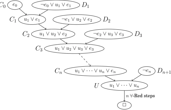
PROPOSITION 3.6. S(Q-ResTFn) = O(n) and CSpace(Q-ResTFn) = O(1), but
w( Q-ResFn) = Ω(n).
PROOF SKETCH. For the upper bounds consider the following proof. Fori∈[n], let
Ci= (u1∨ · · · ∨ui∨ei). Fori∈[n]in sequence, resolvingCi−1andDion variableei−1
gives Ci. ResolvingCn and Dn+1 on variableen gives the clauseU = (u1∨ · · · ∨un).
Finally, applying∀-Red on the clauseU yields the empty clause innmore steps. The proof is depicted in Figure 4.
2 u1∨ · · · ∨un
U
u1∨ · · · ∨un∨en
C
n ¬enD
n+1u1∨u2∨u3∨e3
C
3u1∨u2∨e2
C
2 ¬e2∨u3∨e3D
3u1∨e1
C
1 ¬e1∨u2∨e2D
2e0
C
0 ¬e0∨u1∨e1D
1n∀-Red steps
Fig. 4. Proof of Proposition 3.6: AQ-ResTrefutation of the false QBFFn.
This is a tree-like proof of sizeO(n). Further, each resolution step involves an axiom clause, so at each step we need to pebble just two clauses, and so the space requirement isO(1).
Concerning the width lower bound, by the order of quantification in Fn, every
ex-istential literal in Fn blocks any ∀-reduction. Therefore, in any refutation, when a
∀-reduction is first used, the clauseC has only universal variables. At this point, the empty clause is derivable fromCby a series of∀-reductions. Note that if any clause is dropped fromFn, the resulting QBF is no longer false. Thus any refutation must use
all clauses. HenceCmust have all universal variables in it; it must be(u1∨ · · · ∨un)
as alluivariables have been accumulated, without being reduced. Then clauseC has
widthn.
Noting that w(Fn) = 3, Proposition 3.6 implies that the relationships from
[image:12.612.160.454.292.481.2]As the above example illustrates, it is easy to enforce that universal variables are accumulated in a clause, thus leading to large width. Hence the following question naturally arises: can we obtain size-width or space-width relations by using the tighter measure of only counting existential variables?
This aligns with the situation in the expansion systems AExp+Res and IR-calc, where clauses contain only existential variables. In this respect, it is worth noting that the above example indeed does not demonstrate the failure of the size-width rela-tionship in expansion-based calculi. For instance, inAExp+Res, a tree-like refutation could download the existential variables of axioms annotated withui/0fori∈[n], and
generate the empty clause inO(n)steps with width just 2 at the leaves and 1 at the internal nodes. More formally, consider the assignmentτwhich assigns0to all univer-sal variables ofFn. In
A
Exp+Res, we can download the following clauses, with respect toτ:
Cτ
0 : (e
u1/0,...,un/0
0 )
Fori∈[n], Diτ: (¬e
u1/0,...,un/0
i−1 ∨e
u1/0,...,un/0
i )
Dnτ+1: (¬enu1/0,...,un/0).
Now, the AExp+Resproof ofFn is straightforward: fori ∈ {0,1, . . . , n}, let Eiτ be the
unit clause (eu1/0,...,un/0
i ). Note that E0τ has been downloaded as C0τ. For i ∈ [n], in
sequence, resolve Eτ
i−1 and Dτi on variable e
u1/0,...,un/0
i−1 to derive Eiτ. Finally resolve
Eτ
n andDnτ+1on variablee
u1/0,...,un/0
n to derive the empty clause. Clearly, the size and
width of this proof areO(n)andO(1)respectively.
Thus, to get a consistent and interesting width measure for QBF calculi, we consider the notion of existential width that just counts the number of existential literals. This approach is justified also forQ-Resas the calculus can only resolve on existential variables, and rules out the easy counterexamples above. Formally we define it as follows.
Definition 3.7. Theexistential widthof a clauseCis the number of existential liter-als inC; we denote it byw∃(C). Usingw∃instead ofw, we obtain the existential width of a formulaw∃(F), of a proofw∃(π), and of refuting a false QBFw∃(PF).
For the expansion systemsAExp+ResandIR-calcthe notions of existential width and width of a proof coincide. (In particular, distinct annotations of the same existential variable in a single clause are counted as distinct literals.) Hence we can drop the
∃ subscript in width of proofs in these systems. However, for the width of the input clauses from the QBF under consideration, there is still a difference between the two measureswandw∃, as the QBF may contain universal literals.
4. NEGATIVE RESULTS: SIZE-WIDTH AND SPACE-WIDTH RELATIONS FAIL IN Q-RES
In this section we show that in the Q-Resproof system, even replacing width by ex-istential width, the relations to size or space as in classical resolution (Theorems 3.3 and 3.5) no longer hold for both tree-like and general proofs.
Firstly, we point out where the technique of Ben-Sasson and Wigderson [2001] fails. A crucial ingredient of their proof is the following statement: if a clause A can be derived fromF|x/1in widthw, then the clauseA∨ ¬xcan be derived fromF in width w+ 1 (possibly using a weakening rule at the end). We show that the statement no longer holds inQ-Res.
PROPOSITION 4.1. There are false QBFsFn, with an existential variableb
existential-width proof, but to derive¬bfromFnrequires large existential width inQ-Res. In fact,
Fnitself requires large existential width to refute inQ-Res.
PROOF. The QBF Fn is constructed by taking the conjunction of two QBFs with
distinct variables. The first QBF is a very simple one: ∃a∀u∃b. (a∨u∨ ¬b)∧(¬a). It is true, but if b is set to 1, it becomes false. The second QBF is a false QBF of the form ∃~xGn(~x), where Gn are polynomial-size unsatisfiable CNF formulas over the ~x
variables, such thatGnneeds large width in classical resolution. One such example is
the CNF formula described by Bonet and Galesi [1999], that we denote asBGn.BGn
is an unsatisfiable3-CNF formula overO(n2)variables withw(
ResBGn) = Ω(n). Now
defineFnas:
∃~x∃a∀u∃b. (a∨u∨ ¬b)∧(¬a)∧BGn(~x).
Note that the clauses(a∨u∨¬b)∧(¬a)contain a contradiction if and only ifb= 1. Thus
Fn|b/1can be refuted with existential width 1 using just these two clauses: a∀-Red on
(a∨u)yieldsawhich can be resolved with¬a.
Let us now see how we can derive¬bfromFn. From clausesa∨u∨ ¬band¬awe can
deriveu∨ ¬b, but now we cannot∀-reduceuas it is blocked byb. Therefore we need to expose the contradiction inBGn, derive the empty clause and then use weakening to
obtain¬b. Since all the variables inBGnare existential,Q-Resdegenerates to classical
resolution, requiring (existential) widthΩ(n).
Since settinga=b= 0satisfies the first part of the QBF, and since the two parts of the QBF have disjoint variables, the only way to refuteFnis to expose the contradiction
inBGn, and as discussed above, this requires (existential) widthΩ(n).
The example in the proof of Proposition 4.1 can be made ‘less degenerate’ by inter-leaving more existential and universal variables disjoint from~xand putting them in the first QBF. All we need is thatbis quantified existentially at the end, the first QBF is true as a whole but false ifb= 1, and this latter QBF can be refuted inQ-Reswith small existential width.
We now show that it is not just the technique of Ben-Sasson and Wigderson [2001] that fails for Q-Res. No other technique will work either, because the relation from Theorem 3.3 between size and existential width itself fails to hold. The same example also shows that the relation from Theorem 3.5 between space and existential width also fails to hold.
We first give an example where the relation for tree-like proofs fails. For this we use formulasCRndescribing a natural completion principle, introduced by Janota and
Marques-Silva [2015].4The formulaCR
nis as follows:
CRn=∃x1,1. . . xn,n∀z∃a1. . . an∃b1. . . bn.
Ci,j: (xi,j∨z∨ai), i, j∈[n]
Di,j: (¬xi,j∨ ¬z∨bj), i, j∈[n]
A: _
i∈[n] ¬ai
B: _
i∈[n] ¬bi.
4
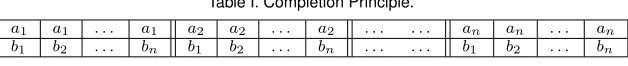
CRnis constructed from a principle called thecompletion principle. Consider two sets
[image:15.612.152.466.140.173.2]A={a1, . . . , an}andB={b1, . . . , bn}, and depict their cross productA×Bas in Table I.
Table I. Completion Principle.
a1 a1 . . . a1 a2 a2 . . . a2 . . . an an . . . an
b1 b2 . . . bn b1 b2 . . . bn . . . b1 b2 . . . bn
The following two-player game is played on Table I. In the first round, player 1 deletes exactly one cell from each column. In the second round, player 2 chooses one of the two rows. Player 2 wins if the chosen row contains either the complete setAor the setB; otherwise player 1 wins. The completion principle states that player 2 has a winning strategy. The false QBFCRnexpresses the notion that player 1 has a winning
strategy. For each column
ai
bj
of the table (denote this the(i, j)thcolumn), there is a
Boolean variable xi,j. Letxi,j = 0denote that player 1 ‘deletesbj’ (i.e., keepsai) from
the (i, j)th column, andx
i,j = 1denotes that player 1 keepsbj in the (i, j)th column.
There is a variablez to denote the choice of player 2: z = 0 means ‘choose top row’. The Boolean variables ai,bj, for i, j ∈ [n]encode that for the chosen values of all the
xk,ℓ, and the row chosen viaz, at least one copy of the elementaiandbjrespectively is
kept. (eg(xi,j∧z)⇒bj).
It is known thatCRnhas a proof of sizeO(n2)inQ-Res, and even inQ-ResT
[Maha-jan and Shukla 2016]. However,CRn has large existential width (i.e.,w∃(CRn) = n),
and for our next result we need a formula with constant initial existential width. To achieve this we proceed similarly as in the Tseitin transformations, i.e., we introduce
2n+ 2new existential variables (i.e.,~y, ~p) at the innermost level inCRn, and replace
the two large clauses inCRn by any CNF formula which preserves their satisfiability.
LetCR′ndenote the modified formula
CR′n=∃x1,1. . . xn,n∀z∃a1. . . an∃b1. . . bn∃y0. . . yn∃p0. . . pn.
Ci,j : (xi,j∨z∨ai), i, j∈[n] (1)
Di,j : (¬xi,j∨ ¬z∨bj), i, j∈[n] (2)
¬y0∧
^
i∈[n]
(yi−1∨ ¬ai∨ ¬yi)∧yn (3)
¬p0∧
^
i∈[n]
(pi−1∨ ¬bi∨ ¬pi)∧pn. (4)
Note thatCR′nhasO(n2)variables andw
∃(CR′n) = 3.
We can use these formulas to refute the size-width and space-width relations in Q-ResT.
THEOREM 4.2. For the above family of QBFs CR′n holds S( Q-ResT CR
′
n) = nO(1),
w∃(CR′n) = 3,CSpace(Q-ResT CR
′
n) =O(1), andw∃(Q-Res CR
′
n)≥n.
PROOF. The clauses ofCR′n, as described above, are partitioned into4groups. For
i∈[4], we call an initial clauseCa type-(i) clause if it belongs to theithgroup. It is clear that from the type-(3) clauses ofCR′n, we can derive the large clauseA=W
i∈[n]¬ai of
CRninn+ 1resolution steps. Similarly we can derive the large clauseB=Wi∈[n]¬biof
CRnfrom the type-(4) clauses inn+ 1steps. The proof refutingCRnuses each of these
large clausesntimes; see below. ThusS(Q-ResT CR
′
n)≤S(Q-ResT CRn) +O(n
We briefly sketch the refutation ofCRn of Mahajan and Shukla [2016] to analyse
its space requirement. The fragmentWj starts with clauseA, successively resolves it
with clauses fromC∗,j to get z∨x1,j ∨ · · · ∨xn,j, eliminatesz through a∀-reduction
to getXj = (x1,j∨ · · · ∨xn,j), then successively resolvesXj with clauses fromD∗,j to
getWj =¬z∨bj. It is easy to see thatO(1)space suffices to construct this fragment.
The overall proof starts with the clauseB, successively resolves it withW1, W2, . . . , Wn
(reusing the space to construct successiveWj’s), and finally gets¬zwhich is eliminated
through a∀-reduction. AgainO(1)space suffices. Refer to Figure 5.
x1,j∨ · · · ∨xn,j Xj
x1,j∨ · · · ∨xn−1,j∨xn,j∨z
x1,j∨ · · · ∨xn−1,j∨xn,j∨z∨ ¬an x
n,j∨z∨an Cn,j
x1,j∨x2,j∨z∨ ¬a3∨ · · · ¬an
x1,j∨z∨ ¬a2∨ · · · ¬an x
2,j∨z∨a2 C2,j ¬a1∨ · · · ∨ ¬an
A x1,j∨z∨a1 C1,j
∀-Red step
(a) AQ-ResTderivation ofXjfrom axiom clausesAandC∗,j
¬z∨bj
Wj
xn,j∨ ¬z∨bj ¬xn,j∨ ¬z∨bj Dn,j
x3,j∨ · · · ∨xn,j∨ ¬z∨bj
x2,j∨ · · · ∨xn,j∨ ¬z∨bj ¬x2,j∨ ¬z∨bj D2,j
x1,j∨x2,j∨ · · ·xn,j
Xj x1,j∨ ¬z∨bj D1,j
(b) AQ-ResTderivation ofWj= (¬z∨bj)from the de-rived clauseXjand axiom clausesD∗,j
2
¬z
¬bn∨ ¬z ¬z∨bn Wn
¬b3∨ · · · ∨ ¬bn∨ ¬z
¬b2∨ ¬b3∨ · · · ∨ ¬bn∨ ¬z ¬z∨b2 W2
¬b1∨b2· · · ∨ ¬bn
B ¬z∨ ¬b1 W1
∀-Red step
(c) Deriving the empty clause from the derived clausesWjand the axiom clauseB
Fig. 5. AQ-ResTrefutation ofCRnfrom [Mahajan and Shukla 2016].
Finally, we show that CR′n needs large existential width to refute, i.e.,
w∃( Q-Res CR ′
n)≥n.
Let π be a proof in Q-Res, πQ-Res CR ′
n. List the clauses of π in sequence, π =
{D0, D1, . . . , Ds=2}, where each clause in the sequence is either a clause fromCR′n, or
is derived from clause(s) preceding it in the sequence using resolution or∀-Red. There must be at least one universal reduction step inπ, since all the initial clauses are nec-essary for refutingCR′n, some of them contain universal variables, and the only way to remove a universal variable inQ-Resis by∀-Red. Lettbe the least index such that in the clauseDt, a∀-Red step has been performed on the only universal variable. Without
[image:16.612.175.437.194.334.2]is identical. As the existential variables~a,~b, ~y, and~pall block the universal variablez, none of them is present in the clauseDt. We use this fact to show thatw∃(Dt)≥n. Our
strategy is to associate some set with each clause inπin a specific way, and use the set size to bound existential width. More formally, we associate a setσwith each clause in
π, and show that the cardinality ofσis large for the clauseDt. We further argue that
Dtcan have a largeσset only if its existential width is large.
We associate the following sets with the literals ofCR′n and the clauses ofπ.
σ(z) = ∅=σ(¬z)
∀i∈[n] σ(ai) = [n]\ {i}={1, . . . , n} \ {i}
∀i∈[n] σ(xi,j) =σ(¬ai) = {i}
∀i∈[n] σ(¬yi) = [n]\[i] ={i+ 1, . . . , n}
∀i∈[n] σ(yi) = [i] ={1, . . . , i}
∀j∈[n] σ(bj) = [n]\ {j}={1, . . . , n} \ {j}
∀j∈[n] σ(¬xi,j) =σ(¬bj) = {j}
∀j∈[n] σ(¬pj) = [n]\[j] ={j+ 1, . . . , n}
∀j∈[n] σ(pj) = [j] ={1, . . . , j}
∀D∈π σ(D) = [
l∈D
σ(l).
The intuition of defining σ in such a way is simple: for all the initial clauses, we want the cardinality of the set σ to be large. Observe that for all clauses C ∈ CR′n,
σ(C) = [n].
Secondly, we want that as long as no∀-Red step has been used, every resolution step must preserve the cardinality ofσ. Observe that for variablesvin~a,~b,~p,~y, the setsσ(v)
andσ(¬v)form a partition of[n]. This helps us in achieving our second goal as follows: forCR′n, we show that any resolution step, before a∀-Red step, must use only one of the variables~a,~b,p~, and~yas a pivot variable. Since the resolvent clause of a resolution rule contains all the literals from the hypothesis except the literals corresponding to the pivot variables, and the literals corresponding to the pivot variables form a partition of[n], the second goal follows.
Finally, we want to show that the existential width of the clauseDtis large. Observe
that we have a singleton setσfor the literalsxi,j, and¬xi,j. We show that the clause
Dtcontains only the literals corresponding to thexi,j variables (along with the only
universal variable being resolved), and sinceDthas a large set (this follows from our
second goal), it must have manyxi,jvariables.
ForD∈π, letπDbe the sub-dag ofπ, rooted atD. Consider the sub-dagπDtofπ. We
have the following observations:
OBSERVATION 4.3. πDt contains at least one type-(1) clause as a source; this is be-causez∈Dt, and the only initial clauses containingzare the type-(1) clauses.
OBSERVATION 4.4. πDt does not contain any clause of type-(2) : asz∈Dt, we know that¬z /∈Dt. Therefore if some type-(2) clause is present in this sub-dag, the only way
to remove ¬z is via∀-Red. This reduction will take place before the reduction onDt,
contradicting our choice of indext. We also conclude that the literal¬z cannot appear anywhere inπDt.
OBSERVATION 4.6. No clause in πDt contains a literal ¬xi,j, since¬xi,j are intro-duced only in type-(2) clauses which were already ruled out.
OBSERVATION 4.7. For any clause C derived solely from type-(3) clauses, σ(C) = [n]. This is true for type-(3) clauses by definition of σ. Using only these clauses, the only resolution step possible is with ay variable as pivot. The claim can be verified by induction on depth: sinceσ(yi)andσ(¬yi)partition[n],[n]\σ(yi)and[n]\σ(¬yi)also
partition[n].
We show that all clauses inπDt that are descendants of some type-(1) clause have
large sets associated with them. In particular, we show:
CLAIM 4.8. Every clause D in πDt such that πD contains a type-(1) clause has
σ(D) = [n].
Deferring the proof briefly, we continue with our argument. From Claim 4.8, we conclude thatσ(Dt) = [n]. Recall that the variables~a,~b, ~y, ~pand the literals¬xi,j are
not present inDt. The only literals left are positivexi,j. These literals are associated
with singleton sets, and the variablesxi,j for different values ofj give the same
sin-gleton set. So we conclude that for each i∈ [n],there must be somexi,j ∈ Dt. Hence
w∃(Dt)≥n.
It remains to establish the claimed set size.
PROOF OF CLAIM4.8. We proceed by induction on the depth of descendants of type-(1) clauses inπDt. The base case is a type-(1) clause itself and follows from the
defini-tion ofσ.
For the inductive step, let D be obtained by resolving(E∨r) and(F ∨ ¬r). There are two cases to consider: both are descendants of some type-(1) clauses, or only one of them, say (E∨r), is a descendant of a type-(1) clause. In the former case, by the induction hypothesis,σ(E∨r) = [n]andσ(F∨¬r) = [n]. In the latter case,σ(E∨r) = [n]
by induction hypothesis, andσ(F∨ ¬r) = [n]from the observations above. ((F∨ ¬r)is not a descendant of any type-(1) clause. But it belongs toπDt which has only type-(1)
and type-(3) clauses. So it must be a descendant of only type-(3) clauses, and hence has
[n]associated with it.)
Thus in both cases, we haveσ(E∨r) =σ(F∨ ¬r) = [n]. So we haveσ(E)⊇[n]\σ(r)
and σ(F) ⊇ [n]\σ(¬r). Observe that the pivot variabler can only be either an~a or a ~y variable. Thus σ(r) and σ(¬r) are disjoint, and hence σ(E)∪σ(F) = [n]. Thus
σ(D) =σ(E)∪σ(F) = [n]as claimed.
This completes the proof of the theorem.
Since tree-like space is at least as large as space, Theorem 4.2 also rules out the space-width relation for general dag-likeQ-Res proofs. However, observe that Theo-rem 4.2 cannot be used to show that the size-existential-width relationship for general dag-like proofs fails inQ-Res, because the QBFsCR′n haveO(n2)variables. However,
we show via another example that the relation fails to hold in Q-Res as well. This example cannot be used for proving Theorem 4.2 because it is known to be hard for Q-ResT [Janota and Marques-Silva 2015]. (Janota and Marques-Silva [2015] show the
hardness forAExp+Res, which implies hardness forQ-ResT, as
A
Exp+Resp-simulates Q-ResT.)
THEOREM 4.9. There is a family of false QBFs φ′
n in O(n) variables such that
S( Q-Resφ
′
n) =nO(1),w∃(φ′n) = 3, andw∃(Q-Resφ
′
PROOF. Consider the following formulas φn, also introduced by Janota and
Marques-Silva [2015]:
φn=∃e1∀u1∃c1c2. . .∃en∀un∃c2n−1c2n.
^
i∈[n]
(¬ei∨c2i−1)∧(¬ui∨c2i−1)∧(ei∨c2i)∧(ui∨c2i)∧
_
i∈[2n] ¬ci
We know from [Janota and Marques-Silva 2015] thatφnhave polynomial-size proofs
inQ-Res (but require exponential-size proofs inQ-ResT). However, in order to prove
Theorem 4.9, we need a formula with constant initial width. To achieve this we con-sider quantified Tseitin transformations ofφn, i.e., we introduce2n+ 1new existential
variables xi at the innermost quantification level in φn, and replace the only large
clause inφn by any CNF formula that preserves satisfiability. Letφ′n denote the
modi-fied formula:
φ′n =∃e1∀u1∃c1c2. . .∃en∀un∃c2n−1c2n∃x0. . . x2n.
^
i∈[n]
(¬ei∨c2i−1)∧(¬ui∨c2i−1)∧(ei∨c2i)∧(ui∨c2i)∧ (5)
¬x0∧
^
i∈[2n]
(xi−1∨ ¬ci∨ ¬xi)∧x2n. (6)
Note thatw∃(φ′n) = 3.
We refer to the clauses in (6) as x-clauses. It is clear that from the x-clauses, we can derive the large clause of φn in 2n+ 1 resolution steps and get back φn. Thus
S( Q-Resφ ′
n)≤S(Q-Resφn) + 2n+ 1 =n
O(1).
We now show that φ′
n needs large existential width. We follow the same strategy
used in proving Theorem 4.2.
Let π be a proof in Q-Res, πQ-Resφ ′
n. List the clauses of π in sequence, π =
{D0, D1, . . . , Ds = 2}, where each clause in the sequence is either a clause fromφ′n,
or is derived from clause(s) preceding it in the sequence using resolution or ∀-Red. There must be at least one universal reduction step in π, since all the initial clauses are necessary for refutingφ′
n, some of them contain universal variables, and the only
way to remove a universal variable inQ-Resis by∀-Red. Letibe the least index such that the clauseDiis obtained by∀-Red onDjfor some0< i. Since allxvariables block
alluvariables,DjandDicannot contain anyxvariables. We use this fact to show that
w∃(Di) = Ω(n). Our strategy is to associate some set with each clause inπin a specific
way, and use the set size to bound existential width. We associate the following sets with the literals ofφ′
nand the clauses ofπ.
σ(x0) = ∅
∀i∈[2n] σ(xi) = [i] ={1,2, . . . , i}
σ(¬x0) = [2n]
∀i∈[2n] σ(¬xi) = [2n]\[i] ={i+ 1, . . . ,2n}
∀i∈[n] σ(ei) =σ(ui) =σ(¬c2i) =σ(c2i−1) = {2i} ∀i∈[n] σ(¬ei) =σ(¬ui) =σ(¬c2i−1) =σ(c2i) = {2i−1}
∀D∈π σ(D) = [
l∈D
σ(l).
Note that for any literalℓ,σ(ℓ)andσ(¬ℓ)are disjoint. The intuition of definingσthis way is as in the proof of Theorem 4.2.
ForD∈π, letπDbe the sub-dag ofπ, rooted atD.
PROOF. The parentDj of node Di contains a universal variable which is then
re-moved through∀-Red to getDi. The universal variables appear only in clauses of
type-(5), but are blocked by thec-variables in every clause where they appear. Thus, before a reduction is permitted, a c-variable must be eliminated by resolution. Since all c -variables appear only positively in type-(5) clauses, somex-clause must be used in the resolution.
We show that all clauses inπDi that are descendants of somex-clause have large
sets associated with them. In particular, we show:
CLAIM 4.11. Every clauseDinπDi such thatπDcontains anx-clause hasσ(D) =
[2n].
Deferring the proof briefly, we continue with our argument. From Claim 4.11, we con-clude that σ(Di) = [2n]. Recall that none of the xvariables belongs toDi. All other
literals are associated with singleton sets, so Di must contains at least2nliterals in
order to be associated with the complete set[2n]. SinceQ-Resproofs prohibit a vari-able and its negation in the same clause, at mostnof the literals inDican be universal
variables. ThusDihas at leastnexistential literals, hencew∃(Di) = Ω(n).
It remains to establish the claimed set size.
PROOF OF CLAIM4.11. We proceed by induction on the depth of descendants ofx -clauses inπDi. The base case is anx-clause itself and follows from the definition ofσ.
For the inductive step, letDbe obtained by resolving(E∨z)and(F∨ ¬z). There are two cases to consider:
Case 1: Both(E∨z)and(F ∨ ¬z)are descendants ofx-clauses (not necessarily the samex-clause). Then by induction,σ(E∨z) = σ(F∨ ¬z) = [2n]. Soσ(E)⊇[2n]\σ(z)
andσ(F) ⊇ [2n]\σ(¬z). Sinceσ(z)andσ(¬z)are disjoint,σ(E)∪σ(F) = [2n]. Thus
σ(D) =σ(E)∪σ(F) = [2n]as claimed.
Case 2: Exactly one of(E∨z)and(F ∨ ¬z)is a descendant of anx-clause. Without loss of generality, letF∨ ¬zbe the descendant. ThenE∨zis either a type-(5) clause or is derived solely from type-(5) clauses using resolution. However, observe that the only clauses derivable solely from type-(5) clauses via resolution, without creating tautolo-gies as mandated inQ-Res, are of the form(c2i−1∨c2i)for somei. It follows thatzis not
anxvariable. Henceσ(z)andσ(¬z)are distinct singleton sets. Further,zcannot be a
uvariable either, since resolution on universal variables is not permitted inQ-Res. Now note that for any type-(5) clause C,σ(C) = {2i−1,2i} for the appropriate i. Similarly,σ(c2i−1∨c2i) ={2i−1,2i}. So ifE∨zis one of these clauses, thenσ(E∨z) =
σ(z)∪σ(¬z) and σ(E) = σ(¬z). Further, as in Case 1, by induction we know that
σ(F∨ ¬z) = [2n]andσ(F)⊇[2n]\σ(¬z). Hence,σ(E∨F) = [2n]as claimed.
This completes the proof of the theorem.
The above counterexamples are provided by formulas that require small size, but large existential width. We will now illustrate via another example that alsolarge size and large width can occur. These examples are very natural formulas based on the parity function, which have recently been used by Beyersdorff et al. [2015] to show exponential size lower bounds forQ-Res, and indeed a separation betweenQ-Resand A
Exp+Res. We will later use these formulas in Section 5 to also show a separation for width betweenQ-ResandAExp+Res.
Letxor(o1, o2, o)be the set of clauses expressingo≡o1⊕o2; that is,{¬o1∨¬o2∨¬o, o1∨ o2∨ ¬o, ¬o1∨o2∨o, o1∨ ¬o2∨o}. In [Beyersdorff et al. 2015], the QBF QPARITYnis
defined as follows:
∃x1· · · ∃xn∀z∃t2· · · ∃tn.xor(x1, x2, t2)∪
[n
The xi variables act as the input for the parity function, and the ti variables are
defined inductively to calculate PARITY(x1, . . . , xi).
We now complement the exponential size lower bound of Beyersdorff et al. [2015] by a width lower bound.
THEOREM 4.12. w∃( Q-ResQPARITYn)≥n.
PROOF. In the formula QPARITYn, the contradiction occurs semantically because of the clausesz∨tn,¬z∨ ¬tn assertingz6=tn (along with the fact that the values of
xvariables uniquely determine the values of all tvariables, in particular, tn). Thus,
at least one of these clauses must be used in any proof, necessitating a ∀-reduction. InQ-Reswe cannot reducez while any of thetvariables are present; and due to the restrictions inQ-Reswe cannot resolve any descendants ofz∨tnwith any descendants
of¬z∨ ¬tnuntil there is at least one∀-reduction.
Consider a smallest Q-Res proof, and assume without loss of generality that a first (lowest) ∀-reduction happens on the positive literal z. Therefore before this ∀ -reduction step we have essentially a resolution proof π from Γ = xor(x1, x2, t2)∪
Sn
i=3xor(ti−1, xi, ti)∪ {tn ∨z}. The clauseD that occurs inπ immediately before the ∀-reduction must only contain variables from{x1, . . . , xn}apart from the literalz, else
the reduction is blocked.
We now use the following observation.
CLAIM 4.13. Supposex1⊕ · · · ⊕xn Cfor some clauseC. ThenC is either a
tau-tology orCcontains all variablesx1, . . . , xn.
PROOF OF CLAIM4.13. Suppose the clause C is not a tautology, but for some nonempty set I ⊂ [n], none of the variables xi with i ∈ I appears in C. Since C is
a non-tautological clause, there is exactly one partial assignment α falsifying C. By setting the variablesxi,i∈I, appropriately, we can increaseαto an assignment
satis-fyingx1⊕ · · · ⊕xn, but still falsifyingC. Hencex1⊕ · · · ⊕xn2C.
Any assignment to thexvariables satisfyingx1⊕ · · · ⊕xnhas a unique extension to
z and thet variables satisfying all clauses of the formula QPARITYn. This extension necessarily has tn = x1⊕ · · · ⊕xn = 1 and z = 0. Since it satisfies all axioms, by
soundness of resolution, it also satisfiesD.
This, along with Claim 4.13, implies thatD is either a tautology or has all x vari-ables. Since it cannot be a tautology (it appears in the proof, and besides, at the very least it has the variable z), it must have all x variables, and hence has existential widthn.
5. SIMULATIONS: PRESERVING SIZE, WIDTH, AND SPACE ACROSS CALCULI
After these strong negative results, ruling out size-width and space-width relations in Q-ResandQ-ResT, we aim to determine whether any positive results hold in the
expansion systemsAExp+ResandIR-calc. Before we can do this we need to relate the measures of size, width, and space across the three calculiQ-Res,AExp+Res,IR-calc. Of course, such a comparison in terms of refined simulations is also interesting in its own as it determines the relative strength of the different proof systems. As size corresponds to running time, and space to memory consumption of QBF solvers, such a comparison yields interesting insights into the power of QBF solvers using CDCL vs. expansion techniques.
It is known thatIR-calcp-simulatesAExp+ResandQ-Res[Beyersdorff et al. 2014], and thatAExp+Resp-simulatesQ-ResT[Janota and Marques-Silva 2015]. We revisit
proofs that are tree-like if the original proof is tree-like. The relationships we establish are stated in the following theorem:
THEOREM 5.1. For all false QBFsF, the following relations hold:
(1) 1
2S( IRT-calcF)≤S( ∀Exp+ResT F)≤S(IRT-calcF)≤3S(Q-ResTF).
(2) w(IR-calcF) =w( ∀Exp+ResF)≤w∃( Q-ResF).
(3) CSpace( ∀Exp+Res
T F) =CSpace( IRT-calcF)≤CSpace( Q-ResTF).
These results follow from Proposition 5.2 and Lemmas 5.3, 5.4 that are stated and established below.
PROPOSITION5.2 (BEYERSDORFF ET AL. [2014]). Any proof inAExp+Resof size S, width W, and space C can be efficiently converted into a proof inIR-calc of size at most2S, widthW, and spaceC. If the proof inAExp+Resis tree-like, so is the resulting
IR-calcproof.
PROOF. InIR-calc, when an axiom is downloaded, the existential literals in it are annotated partially. However inAExp+Res, the annotations arecomplete; all universal variables at a lower level than a literal appear in its annotation. To convert a proofπin A
Exp+Resto one inIR-calc, all that is needed is to follow up each axiom-download with an instantiation that completes the annotations as inπ. This introduces at most one extra step per leaf but does not increase width. Also observe that the space required has not changed: to instantiate a clause we can reuse the same space.
LEMMA 5.3. AExp+ResT p-simulatesIRT-calcwhile preserving its width, size, and
space.
PROOF. Recall the main reason whyIRT-calcproofs differ from those in
A
Exp+ResT: axioms are downloaded with partial rather than complete annotations, and annota-tions can be extended at any stage by theinstoperation.
The idea is to systematically transform an IRT-calc proof, proceeding downwards
from the top where we have the empty clause, and modifying annotations as we go down, so that when all leaves have been modified the resulting proof is in fact an A
Exp+ResTproof. This crucially requires that we start with a tree-like proof; if the un-derlying graph is not a tree, we cannot always find a way of modifying the annotations that will work for all descendants.
Letπbe anIRT-calcproof of a false QBFF. Without loss of generality, we can assume
that every resolution node has, as parent, an instantiation node. (If it does not, we introduce the dummyinst(∅,∗)node between it and its parent.) Since the proof is tree-like, we can also collapse contiguous instantiation nodes into a single instantiation node. Thus, as we move down a path from the root, nodes are alternately instantiation and resolution nodes. We consider each resolution node and its parent instantiation node to be at the same level.
Starting from the top, which we call level zero, we transformπto another proof π′ inIRT-calcmaintaining the following invariants: after theithstep, all the instantiated
clauses up to level iare fully annotated and the instantiating assignments are com-plete. Thus the instantiation steps become redundant. This further implies that after the last level (when we reach the axiom farthest from the top), the resulting proof is in fact aAExp+ResTproof.
![Fig. 1.The rules of Q-Res [Kleine B¨uning et al. 1995]](https://thumb-us.123doks.com/thumbv2/123dok_us/1907064.149061/8.612.110.505.453.565/fig-rules-q-res-kleine-b-uning-et.webp)
![Fig. 5.A Q-ResT refutation of CRn from [Mahajan and Shukla 2016].](https://thumb-us.123doks.com/thumbv2/123dok_us/1907064.149061/16.612.175.437.194.334/fig-q-rest-refutation-crn-mahajan-shukla.webp)
