Code generation in computational neuroscience: a review of tools and techniques.

White Rose Research Online URL for this paper:

http://eprints.whiterose.ac.uk/139152/

Version: Published Version

Article:

Blundell, I., Brette, R., Cleland, T.A. et al. (26 more authors) (2018) Code generation in

computational neuroscience: a review of tools and techniques. Frontiers in

Neuroinformatics, 12. 68. ISSN 1662-5196

https://doi.org/10.3389/fninf.2018.00068

[email protected] https://eprints.whiterose.ac.uk/ Reuse

This article is distributed under the terms of the Creative Commons Attribution (CC BY) licence. This licence allows you to distribute, remix, tweak, and build upon the work, even commercially, as long as you credit the authors for the original work. More information and the full terms of the licence here:

https://creativecommons.org/licenses/

Takedown

If you consider content in White Rose Research Online to be in breach of UK law, please notify us by

Edited by: Arjen van Ooyen, VU University Amsterdam, Netherlands Reviewed by: Astrid A. Prinz, Emory University, United States Richard C. Gerkin, Arizona State University, United States Michael Schmuker, University of Hertfordshire, United Kingdom *Correspondence: Jochen Martin Eppler [email protected]

Received:15 March 2018 Accepted:12 September 2018 Published:05 November 2018 Citation: Blundell I, Brette R, Cleland TA, Close TG, Coca D, Davison AP, Diaz-Pier S, Fernandez Musoles C, Gleeson P, Goodman DFM, Hines M, Hopkins MW, Kumbhar P, Lester DR, Marin B, Morrison A, Müller E, Nowotny T, Peyser A, Plotnikov D, Richmond P, Rowley A, Rumpe B, Stimberg M, Stokes AB, Tomkins A, Trensch G, Woodman M and Eppler JM (2018) Code Generation in Computational Neuroscience: A Review of Tools and Techniques. Front. Neuroinform. 12:68. doi: 10.3389/fninf.2018.00068

Code Generation in Computational

Neuroscience: A Review of Tools and

Techniques

Inga Blundell1_{, Romain Brette}2_{, Thomas A. Cleland}3_{, Thomas G. Close}4_{, Daniel Coca}5_,

Andrew P. Davison6_{, Sandra Diaz-Pier}7_{, Carlos Fernandez Musoles}5_{, Padraig Gleeson}8_,

Dan F. M. Goodman9_{, Michael Hines}10_{, Michael W. Hopkins}11_{, Pramod Kumbhar}12_,

David R. Lester11_{, Bóris Marin}8,13_{, Abigail Morrison}1,7,14_{, Eric Müller}15_{, Thomas Nowotny}16_,

Alexander Peyser7_{, Dimitri Plotnikov}7,17_{, Paul Richmond}18_{, Andrew Rowley}11_,

Bernhard Rumpe17_{, Marcel Stimberg}2_{, Alan B. Stokes}11_{, Adam Tomkins}5_{, Guido Trensch}7_,

Marmaduke Woodman19_{and Jochen Martin Eppler}7_*

1_{Forschungszentrum Jülich, Institute of Neuroscience and Medicine (INM-6), Institute for Advanced Simulation (IAS-6), JARA} BRAIN Institute I, Jülich, Germany,2_{Sorbonne Université, INSERM, CNRS, Institut de la Vision, Paris, France,}3_{Department of} Psychology, Cornell University, Ithaca, NY, United States,4_{Monash Biomedical Imaging, Monash University, Melbourne, VIC,} Australia,5_{Department of Automatic Control and Systems Engineering, University of Sheffield, Sheffield, United Kingdom,} 6_{Unité de Neurosciences, Information et Complexité, CNRS FRE 3693, Gif sur Yvette, France,}7_{Forschungszentrum Jülich,} Simulation Lab Neuroscience, Jülich Supercomputing Centre, Institute for Advanced Simulation, Jülich Aachen Research Alliance, Jülich, Germany,8_{Department of Neuroscience, Physiology and Pharmacology, University College London, London,} United Kingdom,9_{Department of Electrical and Electronic Engineering, Imperial College London, London, United Kingdom,} 10_{Department of Neurobiology, School of Medicine, Yale University, New Haven, CT, United States,}11_{Advanced Processor} Technologies Group, School of Computer Science, University of Manchester, Manchester, United Kingdom,12_{Blue Brain} Project, EPFL, Campus Biotech, Geneva, Switzerland,13_{Centro de Matemática, Computação e Cognição, Universidade} Federal do ABC, São Bernardo do Campo, Brazil,14_{Faculty of Psychology, Institute of Cognitive Neuroscience,}

Ruhr-University Bochum, Bochum, Germany,15_{Kirchhoff-Institute for Physics, Universität Heidelberg, Heidelberg, Germany,} 16_{Centre for Computational Neuroscience and Robotics, School of Engineering and Informatics, University of Sussex,} Brighton, United Kingdom,17_{RWTH Aachen University, Software Engineering, Jülich Aachen Research Alliance, Aachen,} Germany,18_{Department of Computer Science, University of Sheffield, Sheffield, United Kingdom,}19_{Institut de Neurosciences} des Systèmes, Aix Marseille Université, Marseille, France

second is to allow model definitions in a high level interpreted language, although this may limit performance. Recently, a third approach has become increasingly popular: using code generation to automatically translate high level descriptions into efficient low level code to combine the best of previous approaches. This approach also greatly enriches efforts to standardize simulator-independent model description languages. In the past few years, a number of code generation pipelines have been developed in the computational neuroscience community, which differ considerably in aim, scope and functionality. This article provides an overview of existing pipelines currently used within the community and contrasts their capabilities and the technologies and concepts behind them.

Keywords: code generation, simulation, neuronal networks, domain specific language, modeling language

1. INTRODUCTION

All brains are composed of a huge variety of neuron and synapse types. In computational neuroscience we use models for mimicking the behavior of these elements and to gain an understanding of the brain’s behavior by conductingsimulation experiments in neural simulators. These models are usually defined by a set of variables which have either concrete values or use functions and differential equations that describe the temporal evolution of the variables.

A simple but instructive example is the integrate-and-fire neuron model, which describes the dynamics of the membrane potentialV in the following way: whenV is below thespiking threshold θ, which is typically at around −50 mV, the time evolution is governed by a differential equation of the type:

d

dtV=f(V)

wherefis a function that is possibly non-linear.

Once Vreaches its thresholdθ, aspikeis fired andV is set back toEL for a certain time called therefractory period.ELis called theresting potentialand is typically around−70 mV. After this time the evolution of the equation starts again. An important simplification compared to biology is that the exact course of the membrane potential during the spike is either completely neglected or only partially considered in most models. Threshold detection is rather added algorithmically on top of the modeled subthreshold dynamics.

Two of the most common variants of this type of model are thecurrent-based and theconductance-basedintegrate-and-fire models. For the case of the current-based model we have the following general form:

d dtV(t)=

1

τ(EL−V(t))

+ 1

CI(t)+F(V(t)).

Here C is the membrane capacitance, τ the membrane time constant, andItheinput currentto the neuron. Assuming that spikes will be fixed to temporal grid points,I(t) is the sum of

currents generated by all incoming spikes at all grid points in time

ti ≤t scaled by their synaptic weight plus a piecewise constant

functionIextthat models an external input:

I(t)= X

i∈N,ti≤t X

k∈S_ti

Ik(t−ti)+Iext(t)

Stis the set of synapses that deliver a spike to the neuron at time

tandIkis the current that enters the neuron through synapsek.

Fis some non-linear function ofVthat may be zero.

One concrete example is the simple integrate-and-fire neuron with alpha-shaped synaptic input, where F(V) ≡ 0, Ik(t) =

e

τsynte

−t/τsyn _{andτsynis the rise time, which is typically around}

0.2–2.0 ms.

When implementing such models in neural simulators their differential equations must be solved as part of the neuron model implementation. One typical approach is to use a numeric integrator, e.g., a simple Euler method.

For a simulation stepsize hand some given approximation

Vt of V(t), using an Euler method would lead to the following

approximationVt+hofV(t+h):

Vt+h=Vt+h(

1

τ(EL−Vt)+

1

CI(t)).

Publications in computational neuroscience mostly contain descriptions of models in terms of their mathematical equations and the algorithms to add additional behavior such as the mechanism for threshold detection and spike generation. However, if looking at a model implementation and comparing it to the corresponding published model description, one often finds that they are not in agreement due to the complexity and variety of available forms of abstractions of such a transformation (e.g., Manninen et al., 2017, 2018). Using a general purpose programming language to express the model implementation even aggravates this problem as such languages provide full freedom for model developers while lacking the means to guide them in their challenging task due to the absence of neuroscience domain concepts.

compositionality is needed on the abstract mathematical side as well as on the implementation level.

The use of problem-tailored model description languages and standardized simulators is often seen as a way out of the dilemma as they can provide the domain-specificity missing in a general programming language, however often at the cost of restricting the users in their freedom to express arbitrary algorithms.

In other words, engineering complex software systems introduces a conceptual gap between problem domains and solution domains. Model driven development (MDD;France and Rumpe, 2007) aims at closing this gap by using abstract models for the description of domain problems and code generation for creating executable software systems (Kleppe et al., 2003). Early MDD techniques have been already successfully applied in computer science for decades (Davis et al., 2006). These techniques ensure reduced development costs and increased software quality of resulting software systems (Van Deursen and Klint, 1998; Fieber et al., 2008; Stahl et al., 2012). MDD also provides methodological concepts to increase design and development speed of simulation code.

It turns out that MDD is not restricted to the software engineering domain, but can be applied in many science and also engineering domains (Harel, 2005; Topcu et al., 2016). For example, the Systems Biology Markup Language (SBML;

Hucka et al., 2003) from the domain of biochemistry enables modeling of biochemical reaction networks, like cell signaling pathways, metabolic pathways, and gene regulation, and has several software tools that support users with the creation, import, export, simulation, and further processing of models expressed in SBML.

MDD works best if the underlying modeling language fits to the problem domain and thus is specifically engineered for that domain (Combemale et al., 2016). The modeling language must provide modularity in several domains: individual neurons of different behavior must be modeled, time, and geometric abstractions should be available, composition of neurons to large networks must be possible and reuse of neuron models or neuron model fragments must be facilitated.

In the context of computational neuroscience (Churchland et al., 1993) the goal of MDD is to transform complex and abstract mathematical neuron, synapse, and network specifications into efficient platform-specific executable representations. There is no lack of neural simulation environments that are able to simulate models efficiently and accurately, each specializing on networks of different size and complexity. Some of these simulators (e.g., NEST,Gewaltig and Diesmann 2007) have included optimized neural and synaptic models written in low-level code without support for more abstract, mathematical descriptions. Others (e.g., NEURON with NMODL,Hines and Carnevale, 1997,see section 2.7) have provided a separate model description language together with tools to convert these descriptions into reusable model components. Recently, such support has also been added to the NEST simulator via NESTML (Plotnikov et al., 2016,

see section 2.4). Finally, other simulators (e.g., Brian,Goodman 2010, see section 2.1; The Virtual Brain, see section 2.10) include model descriptions as integral parts of the simulation script, transparently converting these descriptions into executable code.

These approaches to model descriptions have been complemented in recent years by various initiatives creating simulator-independent model description languages. These languages completely separate the model description from the simulation environment and are therefore not directly executable. Instead, they provide code generation tools to convert the descriptions into code for target environments such as the ones mentioned above, but also for more specialized target platforms such as GPUs (e.g., GeNN,Yavuz et al., 2016,

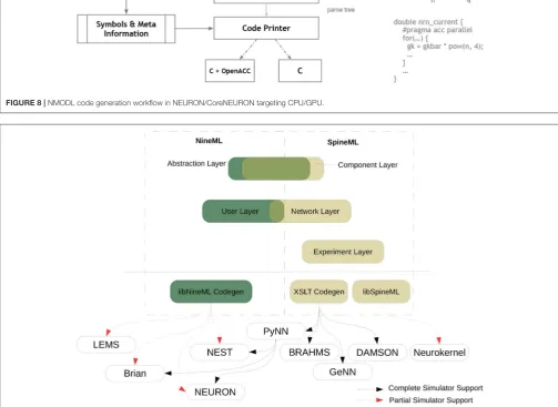
see section 2.2), or neuromorphic chips like SpiNNaker or the BrainScaleS System (see section 3). Prominent description languages include NineML (Raikov et al., 2011, see section 2.6), NeuroML (Goddard et al., 2001; Gleeson et al., 2010), and LEMS (Cannon et al., 2014). These languages are often organized hierarchically, for example LEMS is the low-level description language for neural and synaptic models that can be assembled into a network with a NeuroML description (see section 2.5). Another recently developed description language, SpineML (Richmond et al. 2014, see section 2.8) builds upon LEMS descriptions as well.

A new generation of centralized collaboration platforms like Open Source Brain and the Human Brain Project Collaboratory (see section 3) are being developed to allow greater access to neuronal models for both computationally proficient and non-computational members of the neuroscience community. Here, code generation systems can serve as a means to free the user from installing their own software while still giving them the possibility to create and use their own neuron and synapse models.

This article summarizes the state of the art of code generation in the field of computational neuroscience. In section 2, we introduce some of the most important modeling languages and their code generation frameworks. To ease a comparison of the different technologies employed, each of the sections follows the same basic structure. Section 3 describes the main target platforms for the generation pipelines and introduces the ideas behind the web-based collaboration platforms that are now becoming available to researchers in the field. We conclude by summarizing the main features of the available code generation systems in section 4.

2. TOOLS AND CODE GENERATION

PIPELINES

2.1. Brian

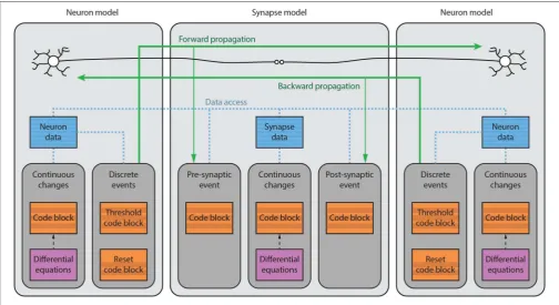
FIGURE 1 |Brian model structure. Brian users define models by specifying equations governing a single neuron or synapse. Simulations consist of an ordered sequence of operations (code blocks) acting on neuronal or synaptic data. A neuronal code block can only modify its own data, whereas a synaptic code block can also modify data from its pre- or post-synaptic neurons. Neurons have three code blocks: one for its continuous evolution (numerical integration), one for checking threshold conditions and emitting spike events, and one for post-spike reset in response to those events. Synapses have three code blocks: two event-based blocks for responding to pre- or postsynaptic spikes (corresponding to forward or backward propagation), and one continuous evolution block. Code blocks can be provided directly, or can be generated from pseudo-code or differential equations.

2.1.1. Main Modeling Focus

Brian focuses on modeling networks of point neurons, where groups of neurons are described by the same set of equations (but possibly differ in their parameters). Depending on the equations, such models can range from variants of the integrate-and-fire model to biologically detailed models incorporating a description of multiple ion channels. The same equation framework can also be used to model synaptic dynamics (e.g., short- and long-term plasticity) or spatially extended, multi-compartmental neurons.

2.1.2. Model Notation

From the user point of view, the simulation consists of components such as neurons and synapses, each of which are defined by equations given in standard mathematical notation. For example, a leaky integrate-and-fire neuron evolves over time according to the differential equation dv/dt = −v/τ. In Brian this would be written as the Python string

'dv/dt=-v/tau : volt' in which the part after the colon

defines the physical dimensions of the variablev. All variables and constants have physical dimensions, and as part of the code generation framework, all operations are checked for dimensional consistency.

Since all aspects of the behavior of a model are determined by user-specified equations, this system offers the flexibility for implementing both standard and non-standard models. For

example, the effect of a spike arriving at a synapse is often modeled by an equation such asvpost←vpost+wwherevpostis the postsynaptic membrane potential andwis a synaptic weight. In Brian this would be rendered as part of the definition of synapses asSynapses(..., on_pre='v_post += w'). However,

the user could as well also change the value of synaptic or presynaptic neuronal variables. For the example of STDP, this might be something like Synapses(..., on_pre='v_post+=w ; Am+=dAm; w=clip(w+Ap, 0, wmax)'), where Am and Ap are

synaptic variables used to keep a trace of the pre- and post-synaptic activity, andclip(x, y, z) is a pre-defined function

(equivalent to the NumPy function of the same name) that returnsxif it is betweenyandz, oryorzif it is outside this

range.

2.1.3. Code Generation Pipeline

Brian code:

G = NeuronGroup(1, 'dv/dt = -v/tau : 1')

“Abstract code” (internal pseudo-code representation)

_v = v*exp(-dt/tau) v = _v

C++ code snippet (scalar part)

const double dt = _ptr_array_defaultclock_dt[0];

const double _lio_1 = exp((-dt)/tau);

C++ code snippet (vector part)

double v = _ptr_array_neurongroup_v[_idx];

const double _v = _lio_1*v; v = _v;

_ptr_array_neurongroup_v[_idx] = v;

Compilable C++ code excerpt:

// scalar code

const double dt = _ptr_array_defaultclock_dt[0];

const double _lio_1 = exp((-dt)/tau);

for(int _idx=0; _idx<_N; idx++) {

// vector code

double v = _ptr_array_neurongroup_v[_idx];

const double _v = _lio_1*v; v = _v;

_ptr_array_neurongroup_v[_idx] = v; }

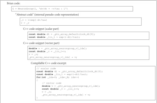
FIGURE 2 |Brian code generation pipeline. Code is transformed in multiple stages: the original Brian code (in Python), with a differential equation given in standard mathematical form; the internal pseudocode or “abstract code” representation (Python syntax), in this case an exact numerical solver for the equations; the C++ code snippets generated from the abstract code; the compilable C++ code. Note that the C++ code snippets include a scalar and vector part, which is automatically computed from the abstract code. In this case, a constant has been pulled out of the loop and named_lio_1.

Such strings or sequences of strings form a sort of mathematical pseudocode called anabstract code block. The user can also specify abstract code blocks directly. For example, to define the operation that is executed upon a spike, the user might write'v_post += w'as shown above.

From an abstract code block, Brian transforms the statements into one of a number of different target languages. The simplest is to generate Python code, using NumPy for vectorized operations. This involves relatively few transformations of the abstract code, mostly concerned with indexing. For example, for a reset operation v ← vr that should be carried out only on those

neurons that have spiked, code equivalent tov[has_spiked] = v_ris generated, wherehas_spikedis an array of integers with

the indices of the neurons that have spiked. The direct C++ code generation target involves a few more transformations on the original code, but is still relatively straightforward. For example, the power operation ab is written asa**b in Python, whereas

in C++ it should be written aspow(a, b). This is implemented

using Python’s built-in AST module, which transforms a string in Python syntax into an abstract syntax tree that can be iterated. Finally, there is the Cython code generation target. Cython is a

Python package that allows users to write code in a Python-like syntax and have it automatically converted into C++, compiled and run. This allows Python users to maintain easy-to-read code that does not have the performance limitations of pure Python.

The result of these transformations is a block of code in a different target language called asnippet, because it is not yet a complete compilable source file. This final transformation is carried out by the widely used Python templating engine Jinja2, which inserts the snippet into a template file.

The final step is the compilation and execution of the source files. Brian operates in one of two main modes: runtime or

that might need to be run repeatedly or for a long duration, these overheads can be significant. Brian therefore also has the standalone mode, in which it generates a complete C++ project that can be compiled and run entirely independently of Python and Brian. This is transparent for the users and only requires them to writeset_device('cpp_standalone')at the beginning

of their scripts. While this mode comes with the advantage of increased performance and portability, it also implies some limitations as user-specified Python code and generated code cannot be interspersed.

Brian’s code generation framework has been designed in a modular fashion and can be extended on multiple levels. For specific models, the user might want to integrate a simulation with hand-written code in the target programming language, e.g., to feed real-time input from a sensor into the simulation. Brian supports this use case by allowing references to arbitrary user-defined functions in the model equations and statements, if its definition in the target language and the physical dimensions of its arguments and result are provided by the user. On a global level, Brian supports the definition of new target languages and devices. This mechanism has for example been used to provide GPU functionality through the Brian2GeNN interface (Nowotny et al., 2014; Stimberg et al., 2014–2018b), generating and executing model code for the GeNN simulator (Yavuz et al., 2016).

2.1.4. Numerical Integration

As stated above, Brian converts differential equations into a sequence of statements that integrate the equations numerically over a single time step. If the user does not choose a specific integration method, Brian selects one automatically. For linear equations, it will solve the equations exactly according to their analytic solution. In all other cases, it will chose a numerical method, using an appropriate scheme for stochastic differential equations if necessary. The exact methods that will be used by this default mechanism depend on the type of the model. For single-compartment neuron and synapse models, the methods exact,

euler, andheun(see explanation below) will be tried in order, and the first suitable method will be applied. Multicompartmental neuron models will chose from the methods exact,exponential euler,rk2, andheun.

The following integration algorithms are provided by Brian and can be chosen by the user:

• exact(namedlinearin previous versions): exact integration for linear equations

• exponential euler: exponential Euler integration for conditionally linear equations

• euler: forward Euler integration (for additive stochastic differential equations using the Euler-Maruyama method) • rk2: second order Runge-Kutta method (midpoint method) • rk4: classical Runge-Kutta method (RK4)

• heun: stochastic Heun method for solving Stratonovich stochastic differential equations with non-diagonal multiplicative noise.

• milstein: derivative-free Milstein method for solving stochastic differential equations with diagonal multiplicative noise

In addition to these predefined solvers, Brian also offers a simple syntax for defining new solvers (for details seeStimberg et al., 2014).

2.1.5. Data and Execution Model

In terms of data and execution, a Brian simulation is essentially just an ordered sequence of code blocks, each of which can modify the values of variables, either scalars or vectors (of fixed or dynamic size). For example,Nneurons with the same equations are collected in a NeuronGroup object. Each variable of the

model has an associated array of length N. A code block will typically consist of a loop over indices i = 0, 1, 2,. . .,N −1 and be defined by a block of code executing in a namespace

(a dictionary mapping names to values). Multiple code objects can have overlapping namespaces. So for example, for neurons there will be one code object to perform numerical integration, another to check threshold crossing, another to perform post-spike reset, etc. This adds a further layer of flexibility, because the user can choose to re-order these operations, for example to choose whether synaptic propagation should be carried out before or after post-spike reset.

Each user defined variable has an associated index variable that can depend on the iteration variable in different ways. For example, the numerical integration iterates over i = 0, 1, 2,. . .,N−1. However, post-spike reset only iterates over the indices of neurons that spiked. Synapses are handled in the same way. Each synapse has an associated presynaptic neuron index, postsynaptic neuron index, and synaptic index and the resulting code will be equivalent tov_post[postsynaptic_index[i]] += w[synaptic_index[i]].

Brian assumes an unrestricted memory model in which all variables are accessible, which gives a particularly flexible scheme that makes it simple to implement many non-standard models. This flexibility can be achieved for medium scale simulations running on a single CPU (the most common use case of Brian). However, especially for synapses, this assumption may not be compatible with all code generation targets where memory access is more restrictive (e.g., in MPI or GPU setups). As a consequence, not all models that can be defined and run in standard CPU targets will be able to run efficiently in other target platforms.

2.2. GeNN

2.2.1. Main Modeling Focus

The focus of GeNN is on spiking neuronal networks. There are no restrictions or preferences for neuron model and synapse types, albeit analog synapses such as graded synapses and gap junctions do affect the speed performance strongly negatively.

1 class MyIzhikevich : public NeuronModels:: Izhikevich

2 {

3 public:

4 DECLARE_MODEL(MyIzhikevich, 5, 2) 5 SET_SIM_CODE(

6 "if ($(V) >= 30.0) {\n" 7 " $(V)=$(c);\n" 8 " $(U)+=$(d);\n" 9 "}\n"

10 "$(V) += 0.5*(0.04*$(V)*$(V)+5.0*$(V)+140.0-$( U)+$(I0)+$(Isyn))*DT;\n"

11 "$(V) += 0.5*(0.04*$(V)*$(V)+5.0*$(V)+140.0-$( U)+$(I0)+$(Isyn))*DT;\n"

12 "$(U) += $(a)*($(b)*$(V)-$(U))*DT;\n"); 13 SET_PARAM_NAMES({"a", "b", "c", "d", "I0"}); 14 };

15 IMPLEMENT_MODEL(MyIzhikevich); 16

17 void modelDefinition(NNmodel &model) 18 {

19 initGeNN();

20 model.setName("SynDelay"); 21 model.setDT(1.0);

22 model.setPrecision(GENN_FLOAT); 23

24 // INPUT NEURONS 25 //==============

26 MyIzhikevich::ParamValues input_p( // Izhikevich parameters - tonic spiking

27 0.02, // 0 - a

28 0.2, // 1 - b 29 -65, // 2 - c 30 6, // 3 - d

31 4.0 // 4 - I0 (input current));

32 MyIzhikevich::VarValues input_ini( // Izhikevich variables - tonic spiking

33 -65, // 0 - V 34 -20 // 1 - U);

35 model.addNeuronPopulation<MyIzhikevich>("Input", 500, input_p, input_ini);

36

37 // OUTPUT NEURONS 38 //===============

39 NeuronModels::Izhikevich::ParamValues output_p( // Izhikevich parameters - tonic spiking

40 0.02, // 0 - a

41 0.2, // 1 - b 42 -65, // 2 - c 43 6 // 3 - d);

44 NeuronModels::Izhikevich::VarValues output_ini( // Izhikevich variables - tonic spiking 45 -65, // 0 - V

46 -20 // 1 - U);

47 PostsynapticModels::ExpCond::ParamValues postExpOut(

48 1.0, // 0 - tau_S: decay time constant for S [ms]

49 0.0 // 1 - Erev: Reversal potential); 50 model.addNeuronPopulation<NeuronModels::

Izhikevich>("Output", 500, output_p, output_ini);

51

52 // INPUT-OUTPUT SYNAPSES 53 //=========================

54 WeightUpdateModels::StaticPulse::VarValues inputOutput_ini(

55 0.03 // 0 - default synaptic conductance); 56

57 model.addSynapsePopulation<WeightUpdateModels:: StaticPulse, PostsynapticModels::ExpCond> 58 ("InputOutput", SynapseMatrixType::

DENSE_GLOBALG, 6, "Input", "Output", {},

59 inputOutput_ini, postExpOut, {});

60 model.finalize(); 61 }

The code example above illustrates the nature of the GeNN API. GeNN expects users to define their own code for neuron and synapse model time step updates as C++ strings. In the example above, the neurons are standard Izhikevich neurons and synaptic connections are pulse coupling with delay. GeNN works with the concept of neuron and synapse types and subsequent definition of neuron and synapse populations of these types.

2.2.2. Code Generation Pipeline

The model description provided by the user is used to generate C++ and CUDA C code for efficient simulation on GPU accelerators. For maximal flexibility, GeNN only generates the code that is specific to GPU acceleration and accepts C/C++ user code for all other aspects of a simulation, even though a number of examples of such code is available to copy and modify. The basic strategy of this workflow is illustrated in

Figure 3. Structuring the simulator framwork in this way allows achieving key goals of code generation in the GPU context. First, the arrangement of neuron and synapse populations into kernel blocks and grids can be optimized by the simulator depending on the model and the hardware detected at compile time. This can lead to essential improvements in the simulation speed. The approach also allows users and developers to define a practically unlimited number of neuron and synapse models, while the final, generated code only contains what is being used and the resulting executable code is lean. Lastly, accepting the users’ own code for the input-output and simulation control allows easy integration with many different usage scenarios, ranging from large scale simulations to using interfaces to other simulation tools and standards and to embedded use, e.g., in robotics applications.

2.2.3. Numerical Integration

Unlike for other simulators, the numerical integration methods, and any other time-step based update methods are for GeNN in the user domain. Users define the code that performs the time step update when defining the neuron and synapse models. If they wish to use a numerical integration method for an ODE based neuron model, users need to provide the code for their method within the update code. This allows for maximal flexibility and transparency of the numerical model updates.

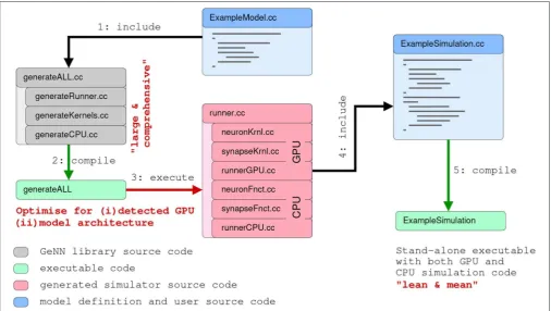
FIGURE 3 |Schematic of the code generation flow for the GPU simulator framework GeNN. Neural models are described in a C/C++ model definition function (“ExampleModel.cc”), either hand-crafted by a user or generated from a higher-level model description language such as SpineML or Brian 2 (see main text). The neuron model description is included into the GeNN compiler that produces optimized CUDA/C++ code for simulating the specified model. The generated code can then be used by hand-crafted or independently generated user code to form the final executable. The framework is minimalistic in generating only optimized CUDA/C++ code for the core model and not the simulation workflow in order to allow maximal flexibility in the deployment of the final executable. This can include exploratory or large scale simulations but also real-time execution on embedded systems for robotics applications. User code in blue, GeNN components in gray, generated CUDA/C++ code in pink.

updates for their neuron models from scratch. For these users there are additional tools that allow connecting other model APIs to GeNN. Brian2GeNN (Nowotny et al., 2014; Stimberg et al., 2014–2018b) allows to execute Brian 2 (see section 2.1Stimberg et al., 2014) scripts with GeNN as the backend and there is a separate toolchain connecting SpineCreator and SpineML (see section 2.8;Richmond et al., 2014) to GeNN to achieve the same. Although there can be a loss in computing speed and the range of model features that can be supported when using such interfaces, using GPU acceleration through Brian2GeNN can be as simple as issuing the commandset_device('genn')in a Python script

for Brian 2.

2.3. Myriad

The goal of the Myriad simulator project (Rittner and Cleland, 2014) is to enable the automatic parallelization and multiprocessing of any compartmental model, particularly those exhibiting dense analog interactions such as graded synapses and mass diffusion that cannot easily be parallelized using standard approaches. This is accomplished computationally via a shared-memory architecture that eschews message-passing, coupled with a radically granular design approach that flattens hierarchically defined cellular models and can subdivide individual isometric

compartments by state variable. Programmatically, end-user models are defined in a Python-based environment and converted into fully-specified C99 code (for CPU or GPU) via code generation techniques that are enhanced by a custom abstract syntax tree (AST) translator and, for NVIDIA GPUs, a custom object specification for CUDA enabling fully on-card execution.

2.3.1. Main Modeling Focus

2.3.2. Model Notation

The core of Myriad is a parallel solver layer designed so that all models that can be represented as a list of isometric, stateful nodes (compartments), can be connected pairwise by any number of arbitrary mechanisms and executed with a high degree of parallelism on CPU threads. No hierarchical relationships among nodes are recognized during execution; hierarchies that exist in user-defined models are flattened during code generation. This flat organization facilitates thread-scaling to any number of available threads and load-balancing with very fine granularity to maximize the utilization of available CPU or GPU cores. Importantly, analog coupling mechanisms such as cable equations, Hodgkin-Huxley membrane channels, mass diffusion, graded synapses, and gap junctions can be parallelized in Myriad just as efficiently as sparse events. Because of this, common hierarchical relationships in neuronal models, such as the positions of compartments along an extended dendritic tree, can be flattened and the elements distributed arbitrarily across different compute units. For example, two nodes representing adjacent compartments are coupled by “adjacency” mechanisms that pass appropriate quantities of charge and mass between them without any explicit or implicit hierarchical relationship. This solver comprises the lowest layer of a three-layer simulator architecture.

A top-level application layer, written in idiomatic Python 3 enriched with additional C code, defines the object properties and primitives available for end-user model development. It is used to specify high-level abstractions for neurons, sections, synapses, and network properties. The mechanisms (particles, ions, channels, pumps, etc.) are user-definable with object-based inheritance, e.g., channels inherit properties based on their permeant ions. Simulations are represented as objects to facilitate iterative parameter searches and reproducibility of results. The inheritance functionality via Python’s native object system allows access to properties of parent component and functionality can be extended and overridden at will.

The intermediate interface layer flattens and translates the model into non-hierarchical nodes and coupling mechanisms for the solver using AST-to-AST translation of Python code to C. Accordingly, the top-level model definition syntax depends only on application-layer Python modules; in principle, additional such modules can be written for applications outside neuroscience, or to mimic the model definition syntax of other Python-based simulators. For the intended primary application of solving dense compartmental models of neurons and networks, the models are defined in terms of their cellular morphologies and passive properties (e.g., lengths, diameters, cytoplasmic resistivity) and their internal, transmembrane, and synaptic mechanisms. State variables include potentials, conductances, and (optionally) mass species concentrations. Equations for mechanisms are arbitrary and user-definable.

2.3.3. Code Generation Pipeline

To achieve an efficient parallelization of dense analog mechanisms, it was necessary to eschew message-passing. Under message-based parallelization, each data transfer between compute units generates a message with an uncertain arrival

time, such that increased message densities dramatically increase the rollback rate of speculative execution and quickly become rate-limiting for simulations. Graded connections such as analog synapses or cable equations yield new messages at every timestep and hence parallelize poorly. This problem is generally addressed by maintaining coupled analog mechanisms on single compute units, with parallelization being limited to model elements that can be coupled via sparse boolean events, such as action potentials (Hines and Carnevale, 2004). Efficient simulations therefore require a careful, platform-specific balance between neuronal complexity and synaptic density (Migliore et al., 2006). The unfortunate consequence is that platform limitations drive model design.

In lieu of message passing, Myriad is based on a uniform memory access (UMA) architecture. Specifically, every mechanism reads all parameters of interest from shared memory, and writes its output to shared memory, at every fixed timestep. Shared memory access, and a global clock that regulates barrier synchronization among all compute units (thereby coordinating all timesteps), are GPU hardware features. For parallel CPU simulations, the OpenMP 3.1+ API for shared-memory multiprocessing has implicit barrier and reduction intrinsics that provide equivalent, platform-independent functionality. Importantly, while this shared-memory design enables analog interactions to be parallelized efficiently, to take proper advantage of this capacity on GPUs, the simulation must execute on the GPU independently rather than being continuously controlled by the host system. To accomplish this, Myriad uses a code generation strategy embedded in its three-layer architecture (see section 2.3.2). The lowest (solver) layer is written in C99 for both CPUs and NVIDIA GPUs (CUDA). The solver requires as input a list of isometric nodes and a list of coupling mechanisms that connect pairs of nodes, all with fully explicit parameters defined prior to compilation (i.e., execution of a Myriad model requires just-in-time compilation of the solver). To facilitate code reuse and inheritance from the higher (Python) layers, a custom-designed minimal object framework implemented in C (Schreiner, 1999) supports on-device virtual functions; to our knowledge this is the first of its kind to execute on CUDA GPUs. The second, or interface, layer is written in Python; this layer defines top-level objects, instantiates the node and mechanism dichotomy, converts the Python objects defined at the top level into the two fully-specified lists that are passed to the solver, and manages communication with the simulation binaries. The top, or application layer, will comprise an expandable library of application-specific modules, also written in Python. These modules specify the relevant implementations of Myriad objects in terms familiar to the end user. For neuronal modeling, this could include neurite lengths, diameters, and branching, permeant ions (mass and charge), distributed mechanisms (e.g., membrane channels), point processes (e.g., synapses), and cable equations, among other concepts common to compartmental simulators. Additional top-layer modules can be written by end users for different purposes, or to support different code syntaxes.

two Python lists of node and mechanism objects. Parameters are resolved, and the Python object lists are transferred to the solver layer via a custom-built Python-to-C pseudo-compiler (pycast; an AST-to-AST translator from Python’s native abstract syntax tree (AST) to the AST of pycparser (a Myriad dependency), facilitated by Myriad’s custom C object framework). These objects are thereby rendered into fully explicit C structs which are compiled as part of the simulation executable. The choice of CPU or GPU computation is specified at execution time via a compiler option. On CPUs and compliant GPUs, simulations execute using dynamic parallelism to maximize core utilization (via OpenMP 3.1+ for CPUs or CUDA 5.0+ on compute capability 3.5+ GPUs).

The limitation of Myriad’s UMA strategy is scalability. Indeed, at its conception, Myriad was planned as a simulator on the intermediate scale between single neuron and large network simulations because its shared-memory, barrier synchronization-dependent architecture limited the scale of simulations to those that could fit within the memory of a single high-speed chassis (e.g., up to the memory capacity of a single motherboard or CUDA GPU card). However, current and projected hardware developments leveraging NVIDIA’s NVLink interconnection bus (NVIDIA Corporation, 2014) are likely to ease this limitation.

2.3.4. Numerical Integration

For development purposes, Myriad supports the fourth-order Runge-Kutta method (RK4) and the backward Euler method. These and other methods will be benchmarked for speed, memory requirements, and stability prior to release.

2.4. NESTML

NESTML (Plotnikov et al., 2016; Blundell et al., 2018; Perun et al., 2018a) is a relatively new modeling language, which currently only targets the NEST simulator (Gewaltig and Diesmann, 2007). It was developed to address the maintainability issues that followed from a rising number of models and model variants and ease the model development for neuroscientists without a strong background in computer science. NESTML is available unter the terms of the GNU General Public License v2.0 on GitHub (https://github.com/nest/nestml;Perun et al., 2018b) and can serve as a well-defined and stable target platform for the generation of code from other model description languages such as NineML (Raikov et al., 2011) and NeuroML (Gleeson et al., 2010).

2.4.1. Main Modeling Focus

The current focus of NESTML is on integrate-and-fire neuron models described by a number of differential equations with the possibility to support compartmental neurons, synapse models, and also other targets in the future.

1 neuron iaf_curr_alpha: 2

3 initial_values:

4 V_m mV = E_L

5 end

6

7 equations:

8 shape I_alpha = (e / tau_syn) * t * exp(-t / tau_syn)

9 I pA = convolve(I_alpha, spikes) 10 V_m' = -1/tau * (V_m - E_L) + I/C_m

11 end

12

13 parameters:

14 C_m pF = 250pF # Capacity of

the membrane

15 Tau ms = 10ms # Membrane time constant.

16 tau_syn ms = 2ms # Time constant

of synaptic current.

17 ref_timeout ms = 2ms # Duration of

refractory period in ms.

18 E_L mV = -70mV # Resting

potential.

19 V_reset mV = -70mV - E_L # Reset

potential of the membrane in mV.

20 Theta mV = -55mV - E_L # Spike

threshold in mV.

21 ref_counts integer = 0 # counter for

refractory steps 22

23 end

24

25 internals:

26 timeout_ticks integer = steps(ref_timeout) # refractory time in steps

27 end

28

29 input:

30 spikes <- spike

31 end

32

33 output: spike

34

35 update:

36 if ref_counts == 0: # neuron not refractory 37 integrate_odes()

38 if V_m >= Theta: # threshold crossing

39 ref_counts = timeout_ticks

40 V_m = V_reset

41 emit_spike()

42 else

43 ref_counts = -1

44 end

45

46 end

47 48 end

The code shown in the listing above demonstrates the key features of NESTML with the help of a simple current-based integrate-and-fire neuron with alpha-shaped synaptic input as described in section 1. A neuron in NESTML is composed of multiple blocks. The whole model is contained in a neuron

block, which can have three different blocks for defining model variables: initial_values, parameters, and internals. Variable declarations are composed of a non-empty list of variable names followed by their type. Optionally, initialization expressions can be used to set default values. The type can either be a plain data type such as integer and real, a physical unit (e.g., mV) or a composite physical unit (e.g.,nS/ms).

block. Postsynaptic shapes and synonyms inside theequations

block can be used to increase the expressiveness of the specification.

The type of incoming and outgoing events are defined in theinputandoutputblocks. The neuron dynamics are specified inside theupdateblock. This block contains an implementation of the propagation step and uses a simple embedded procedural language based on Python.

2.4.2. Code Generation Pipeline

In order to have full freedom for the design, the language is implemented as an external domain specific language (DSL;van Deursen et al., 2000) with a syntax similar to that of Python. In contrast to an internal DSL an external DSL doesn’t depend syntactically on a given host language, which allows a completely customized implementation of the syntax and results in a design that is tailored to the application domain.

Usually external DSLs require the manual implementation of the language and its processing tools. In order to avoid this task, the development of NESTML is backed by the language workbench MontiCore (Krahn et al., 2010). MontiCore uses context-free grammars (Aho et al., 2006) in order to define the abstract and concrete syntax of a DSL. Based on this grammar, MontiCore creates classes for the abstract syntax (metamodel) of the DSL and parsers to read the model description files and instantiate the metamodel.

NESTML is composed of several specialized sublanguages. These are composed through language embedding and a language inheritance mechanism: UnitsDSL provides all data types and physical units, ExpressionsDSL defines the style of Python compatible expressions and takes care of semantic checks for type correctness of expressions, EquationsDSL provides all means to define differential equations and postsynaptic shapes andProceduralDSLenables users to specify parts of the model in the form of ordinary program code. In situations where a modeling intent cannot be expressed through language constructs this allows a more fine-grained control than a purely declarative description could.

The decomposition of NESTML into sublanguages enables an agile and modular development of the DSL and its processing infrastructure and independent testing of the sublanguages, which speeds up the development of the language itself. Through the language composition capabilities of the MontiCore workbench the sublanguages are composed into the unified DSL NESTML.

NESTML neurons are stored in simple text files. These are read by a parser, which instantiates a corresponding abstract syntax tree (AST). The AST is an instance of the metamodel and stores the essence of the model in a form which is easily processed by a computer. It completely abstracts the details of the user-visible model representation in the form of its concrete syntax. The symbol table and the AST together provide a semantic model.

Figure 4 shows an excerpt of the NESTML grammar and explains the derivation of the metamodel. A grammar is composed of a non-empty set of productions. For every production a corresponding class in the metamodel is created.

Based on the right hand side of the productions attributes are added to this class. Classes can be specified by means of specifications of explicit names in the production names of attributes in the metamodel.

NEST expects a model in the form of C++ code, using an internal programming interface providing hooks for parameter handling, recording of state variables, receiving and sending events, and updating instances of the model to the next simulation time step. The NESTML model thus needs to be transformed to this format (Figure 5).

For generating the C++ code for NEST, NESTML uses the code generation facilities provided by the MontiCore workbench, which are based on the template engine Freemarker (https:// freemarker.apache.org/). This approach enables a tight coupling of the model AST and the symbol table, from which the code is generated, with the text based templates for the generation of code.

Before the actual code generation phase, the AST undergoes several model to model transformations. First, equations and shapes are extracted from the NESTML AST and passed to an analysis framework based on the symbolic math package SymPy (Meurer et al., 2017). This framework (Blundell et al., 2018) analyses all equations and shapes and either generates explicit code for the update step or code that can be handled by a solver from the GNU Scientific Library (https://gnu.org/software/gsl/). The output of the analysis framework is a set of model fragments which can again be instantiated as NESTML ASTs and integrated into the AST of the original neuron and replace the original equations and shapes they were generated from.

Before writing the C++ code, aconstant foldingoptimization is performed, which uses the fact that internal variables in NESTML models do not change during the simulation. Thus, expressions involving only internal variables and constants can be factored out into dedicated expressions, which are computed only once in order to speed up the execution of the model.

2.4.3. Numerical Integration

NESTML differentiates between different types of ODEs. ODEs are categorized according to certain criteria and then assigned appropriate solvers. ODEs are solved either analytically if they are linear constant coefficient ODEs and are otherwise classified as stiff or non stiff and then assigned either an implicit or an explicit numeric integration scheme.

2.5. NeuroML/LEMS

FIGURE 4 |Example definition of a NESTML concept and generation of the AST.(Left)A production for a function in NESTML. The lefthandside defines the name of the production, the righthandside defines the production using terminals, other productions and special operators (*,?). A function starts with the keyword

functionfollowed by the function’s name and an optional list of parameters enclosed in parentheses followed by the optional return value. Optional parts are marked with?. The function body is specified by the production (Block) between two keywords.(Right)The corresponding automatically derived meta-model as a class diagram. Every production is mapped to an AST class, which is used in the further language processing steps.

FIGURE 5 |Components for the code generation in NESTML.(Top)Source model, corresponding AST, and helper classes.(Middle)Templates for the generation of C++ code. The left template creates a C++ class body with an embedded C++ struct, the right template maps variable name and variable type using a helper class. The template on the left includes the template on the right once for each state variable defined in the source model.(Bottom)A C++ implementation as created from the source model using the generation templates.

Carnevale and Hines, 2006; GENESIS;Bower and Beeman, 1998) in order for the models to be simulated.

Nevertheless, the need for greater flexibility and extensibility beyond a predefined set of components and, more importantly, a demand for lower level model descriptions also described in a standardized format (contrarily to NeuroML1, where for example component dynamics were defined textually in the language reference, thus inaccessible from code) culminated in a

major language redesign (referred to asNeuroML2), underpinned by a second, lower level language called Low Entropy Model Specification(LEMS;Cannon et al., 2014).

2.5.1. Main Modeling Focus

differential equations, plus discrete state jumps or changes in dynamical regimes mediated by state-dependent events—also known asHybrid Systems(van der Schaft and Schumacher, 2000).

NeuroML2 is thus a DSL (in the computational neuroscience domain) defined usingLEMS, and as such provides standardized, structured descriptions of model dynamics up to the ODE level.

2.5.2. Model Notation

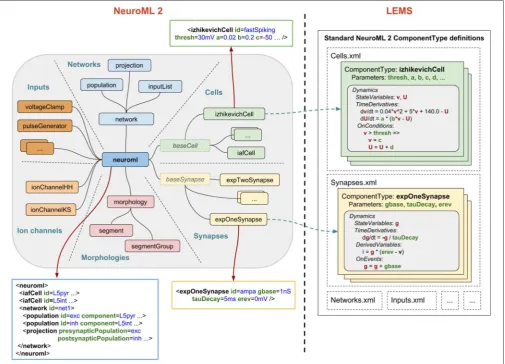
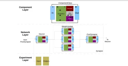
An overview of NeuroML2and LEMSis depicted inFigure 6, illustrating how Components for an abstract cell model (izhikevichCell) and a synapse model (expOneSynapse) can be specified in XML (i.e., in the computational neuroscience domain, only setting required parameters for theComponents), with the definitions for their underlying models specified in

LEMS ComponentTypeswhich incorporate a description of the dimensions of the parameters, the dynamical state variables and behavior when certain conditions or events occur.

Besides providing more structured information describing a given model and further validation tools for building new ones (Cannon et al., 2014),NeuroML2-LEMSmodels can be directly parsed, validated, and simulated via the jLEMS interpreter (Cannon et al., 2018), developed in Java.

2.5.3. Code Generation Pipeline

Being derived fromLEMS, a metalanguage designed to generate simulator-agnostic domain-specific languages, NeuroML2 is prone to be semantically different at varying degrees from potential code generation targets. As discussed elsewhere in the

present article (sections 2.1 and 2.4), code generation boils down to trivial template merging or string interpolation once the source and target models sit at comparable levels of abstraction (reduced “impedance mismatch”), implying that a number of semantic processing steps might be required in order to transform

LEMS/NeuroML2into each new target. GivenLEMS/NeuroML2’s low-level agnosticism—there is always the possibility that it will be used to generate code for a yet-to-be-invented simulator—

NeuroML2infrastructure needs to be flexible enough to adapt to different strategies and pipelines.

This flexibility is illustrated in Figure 7, where NeuroML2

pipelines involving code generation are outlined. Three main strategies are discussed in detail: a procedural pipeline starting fromjLEMS’s internal structures (Figure 7P), which as the first one to be developed, is the most widely tested and supports more targets; a pipeline based on building an intermediate representation semantically similar to that of typical neuronal modeling / hybrid-system-centric numerical software, which can then be merged with templates (as decoupled as possible from LEMS internals) for each target format (Figure 7T); and a customizable language binding generator, based on an experimental compiler infrastructure forLEMSwhich provides a rich semantic model with validation and automatic generation of traversers (Figure 7S)—akin to semantic models built by language workbenches such as MontiCore, which has been employed to build NESTML (section 2.4).

2.5.3.1. jLEMS runtime and procedural generation

The jLEMS simulator was built alongside the development of theLEMSlanguage, providing a testbed for language constructs and, as such, enables parsing, validating, and interpreting of

LEMSdocuments (models). LEMS is canonically serialized as

XML, and the majority of existing models have been directly developed using this syntax. In order to simulate the model,

jLEMS builds an internal representation conforming toLEMS

semantics (Cannon et al., 2014). This loading of theLEMS XML

into this internal state is depicted as a green box in theP(middle) branch ofFigure 7. Given that any neuronal or general-purpose simulator will eventually require similar information about the model in order to simulate it, the natural first approach to code generation fromLEMSinvolved procedural interaction with this internal representation, manually navigating through component hierarchies to ultimately fetch dynamics definitions in terms of

Parameters,DerivedVariables, and routing events. Exporters from

NeuroML2toNEURON(bothhocandmod),Brian1andSBML

were developed using these techniques (end point ofFigure 7 P), and can be found in the org.neuroml.export repository (Gleeson et al., 2018).

Even if all the information required to generate code for different targets is encoded in the jLEMS intermediate representation, the fact that the latter was designed to support a numerical simulation engine creates overheads for the procedural pipeline, typically involving careful mixed use ofLEMS/ domain

abstractions and requiring repetitive application of similar traversal/conversion patterns for every new code generator. This regularity suggested pursuing a second intermediate representation, which would capture these patterns into a further abstraction.

2.5.3.2. Lower-level intermediate representation/templating

Neuronal simulation engines such asBrian,GENESIS,NESTand

NEURONtend to operate at levels of abstraction suited to models described in terms of differential equations (e.g., explicit syntax for time derivatives inBrian,NESTMLandNEURONnmodl), in conjunction with discontinuous state changes (usually abstracted within “event handlers” in neuronal simulators). Code generation for any of those platforms from LEMS model would thus be facilitated if LEMS models could be cast at this level of abstraction, as most of the transformations would consist of one-to-one mappings which are particularly suited for template-based generation. Not surprisingly, Component dynamics in LEMS

are described precisely at the hybrid dynamical system level, motivating the construction of a pipeline (Figure 7 T) centered around an intermediate representation, termeddLEMS(Marin et al., 2018b), which would facilitate simplified code generation not only for neuronal simulators (dLEMS being semantically close to e.g.,BrianandNESTML) but also for ODE-aware general purpose numerical platforms like Matlab or even C/Sundials

(Hindmarsh et al., 2005).

Besides reducing development time by removing complex logic from template bodies—all processing is done on the semantic model, using a general purpose language (Javain the case ofjLEMSbacked pipelines) instead of the templating DSL, which also promotes code reuse—this approach also enables target language experts to work with templates with reduced syntactic noise, shifting focus from processing information on

LEMSinternals to optimized generation (e.g., more idiomatic, efficient code).

2.5.3.3. Syntax oriented generation/semantic model construction

Both the procedural and template-based pipelines (Figure 7 P,T) described in the preceding paragraphs stem from the jLEMS internal representation data structure, which is built from both theLEMSdocument and an implementation ofLEMSsemantics, internal tojLEMS. To illustrate the interplay between syntax and semantics, consider for example the concept ofComponentType extension in LEMS, whereby a ComponentType can inherit structure from another. In a LEMS document serialized as

XML, the “child” ComponentType is represented by an XML element, with an attribute (string) containing the name of the “parent.” Syntactically, there is no way of determining that this string should actually represent an existingComponentType, and that structure should be inherited—that is the role of semantic analysis.

The Pand T pipelines rely heavily on APIs for traversing, searching, and transforming a semantic model. They have been implemented on top of the one implemented by jLEMS— even though it contains further transformations introduced to ease interpretation of models for numerical simulation—the

original purpose ofjLEMS. Given that both code generation and interpretation pipelines depend on the initial steps of parsing the concrete syntax (XML) and building a semantic model with novel APIs, a third “semantic” pipeline (Figure 7 S) is under development to factor out commonalities. Starting withLEMS

definitions for a domain-specific language—in the particular case of NeuroML2, a collection of ComponentTypes spanning the domain of biophysical neuronal models—a semantic model is produced in the form of domain types for the target language, via template-based code generation. Any (domain specific, e.g.,

NeuroML2) LEMS document can then be unmarshalled into domain objects, constituting language bindings with custom APIs that can be further processed for code generation or used in an interpreter.

Any LEMS-backed language definition (library of

ComponentTypes) can use the experimental Java binding generator directly through a Maven plugin we have created (Marin and Gleeson, 2018). A sample project where domain classes forNeuroML2are built is available (Marin et al., 2018a), illustrating how to use the plugin.

2.5.3.4. Numerical integration

As a declarative model specification language, LEMS was designed to separate model description from numerical implementation. When building a model usingLEMS—or any DSL built on top of it such asNeuroML2—the user basically instantiates preexisting (or creates new and then instantiates)

LEMS ComponentTypes, parameterizing and connecting them together hierarchically. In order to simulate this model, it can either be interpreted by the native LEMS interpreters (e.g., jLEMS, which employs either Forward-Euler or a 4th order Runge-Kutta scheme to approximate solutions for ODE-based node dynamics and then performs event detection and propagation) or transform the models to either general-purpose languages or domain-specific simulators, as described above for each code generation pipeline.

2.5.4. General Considerations and Future Plans

Different code generation strategies for LEMS based domain languages —such as NeuroML2—have been illustrated. With

LEMSbeing domain and numerical implementation agnostic, it is convenient to continue with complementary approaches to code generation, each one fitting different users’ requirements. The first strategy to be developed, fully procedural generation based on jLEMS internal representation (P), has lead to the most complex and widely tested generators to date—such as the one fromNeuroML2toNEURON(mod/hoc). Given that

jLEMS was not built to be a high-performance simulator, but a reference interpreter compliant with LEMS semantics, it is paramount to have robust generation for state-of-the art domain-specific simulators if LEMS-based languages are to be more widely adopted. Conversely, it is important to lower the barriers for simulator developers to adoptLEMS-based models as input. These considerations have motivated building the

dLEMS/templating based code generation pipeline (T), bringing

relate to templates resembling the native format, with minimal interaction withLEMSinternals.

The semantic-model/custom API strategy (S) is currently at an experimental stage, and was originally designed to factor out parsing/semantic analysis from jLEMS into a generic compiler front end-like (Grune et al., 2012) standalone package. This approach was advantageous in comparison with the previous XML-centric strategy, where bindings were generated from XML Schema Descriptions manually built and kept up-to-date with LEMS ComponentType definitions—which incurred in redundancy as ComponentTypes fully specify the structure of a domain document (Component definitions). While it is experimental, the modular character of this new infrastructure should contribute to faster, more reusable development of code generators for new targets.

2.6. NineML, Pype9, 9ML-Toolkit

The Network Interchange for NEuroscience Modeling Language (NineML) (Raikov et al., 2011) was developed by the International Neuroinformatics Coordinating Facility (INCF) NineML taskforce (2008–2012) to promote model sharing and reusability by providing a mathematically-explicit, simulator-independent language to describe networks of point neurons. Although the INCF taskforce ended before NineML was fully specified, the component-based descriptions of neuronal dynamics designed by the taskforce informed the development of both LEMS (section 2.5;Cannon et al., 2014) and SpineML (section 2.8;Richmond et al., 2014), before the NineML Committee (http://nineml.net/committee) completed version 1 of the specification in 2015 (https://nineml-spec.readthedocs.io/ en/1.1).

NineML only describes the model itself, not solver-specific details, and is therefore suitable for exchanging models between a wide range of simulators and tools. One of the main aims of the NineML Committee is to encourage the development of an eco-system of interoperable simulators, analysis packages, and user interfaces. To this end, the NineML Python Library (https://nineml-python.readthedocs.io) has been developed to provide convenient methods to validate, analyse, and manipulate NineML models in Python, as well as handling serialization to and from multiple formats, including XML, JSON, YAML, and HDF5. At the time of publication, there are two simulation packages that implement the NineML specification using code generation, PYthon PipelinEs for 9ml (Pype9; https://github. com/NeuralEnsemble/pype9) and the Chicken Scheme 9ML-toolkit (https://github.com/iraikov/9ML-9ML-toolkit), in addition to a toolkit for dynamic systems analysis that supports NineML through the NineML Python Library, PyDSTool (Clewley, 2012).

2.6.1. Main Modeling Focus

The scope of NineML version 1 is limited to networks of point neurons connected by projections containing post-synaptic response and plasticity dynamics. However, version 2 will introduce syntax to combine dynamic components (support for “multi-component” dynamics components, including their flattening to canonical dynamics components, is already implemented in the NineML Python Library), allowing neuron

models to be constructed from combinations of distinct ion channel and concentration models, that in principle could be used to describe models with a small number of compartments. Explicit support for biophysically detailed models, including large multi-compartmental models, is planned to be included in future NineML versions through a formal “extensions” framework.

2.6.2. Model Notation

NineML is described by an object model. Models can be written and exported in multiple formats, including XML, JSON, YAML, HDF5, Python, and Chicken Scheme. The language has two layers, the Abstraction layer (AL), for describing the behavior of network components (neurons, ion channels, synapses, etc.), and theUser layer, for describing network structure. The AL represents models of hybrid dynamical systems using a state machine-like object model whose principle elements areRegimes, in which the behavior of the model state variables is governed by ordinary differential equations, and Transitions, triggered by conditions on state variable values or by external event signals, and which cause a change to a new regime, optionally accompanied by a discontinuous change in the values of state variables. For the example of a leaky integrate-and-fire model there are two regimes, one for the subthreshold behavior of the membrane potential, and one for the refractory period. The transition from subthreshold to refractory is triggered by the membrane potential crossing a threshold from below, and causes emission of a spike event and reset of the membrane potential; the reverse transition is triggered by the time since the spike passing a threshold (the refractory time period). This is expressed using YAML notation as follows:

1 NineML:

2 '@namespace': http://nineml.net/9ML/1.0 3 ComponentClass:

4 - name: LeakyIntegrateAndFire

5 Parameter:

6 - {name: R, dimension: resistance}

7 - {name: refractory_period, dimension: time} 8 - {name: tau, dimension: time}

9 - {name: v_reset, dimension: voltage} 10 - {name: v_threshold, dimension: voltage}

11 AnalogReducePort:

12 - {name: i_synaptic, dimension: current, operator: +}

13 EventSendPort:

14 - {name: spike_output}

15 AnalogSendPort:

16 - {name: refractory_end, dimension: time} 17 - {name: v, dimension: voltage}

18 Dynamics:

19 StateVariable:

20 - {name: refractory_end, dimension: time}

21 - {name: v, dimension: voltage}

22 Regime:

23 - name: refractory

24 OnCondition:

25 - Trigger: {MathInline: t > refractory_end }

26 target_regime: subthreshold

27 - name: subthreshold