Fragmentation and disk formation during high-mass star formation. IRAM NOEMA (Northern Extended Millimeter Array) large program CORE

Astronomy

_&

Astrophysics

© ESO 2018

Fragmentation and disk formation during high-mass

star formation

IRAM NOEMA (Northern Extended Millimeter Array) large program CORE

H. Beuther

, J. C. Mottram

, A. Ahmadi

, F. Bosco

, H. Linz

, Th. Henning

, P. Klaassen

, J. M. Winters

, L. T. Maud

,

R. Kuiper

_{, D. Semenov}

_{, C. Gieser}

_{, T. Peters}

_{, J. S. Urquhart}

_{, R. Pudritz}

_{, S. E. Ragan}

_{, S. Feng}

_{, E. Keto}

_,

S. Leurini

, R. Cesaroni

, M. Beltran

, A. Palau

, Á. Sánchez-Monge

, R. Galvan-Madrid

, Q. Zhang

, P. Schilke

,

F. Wyrowski

_{, K. G. Johnston}

_{, S. N. Longmore}

_{, S. Lumsden}

_{, M. Hoare}

_{, K. M. Menten}

_{, and T. Csengeri}

1 _{Max Planck Institute for Astronomy, Königstuhl 17, 69117 Heidelberg, Germany}

e-mail:[email protected]

2 _{UK Astronomy Technology Centre, Royal Observatory Edinburgh, Blackford Hill, Edinburgh EH9 3HJ, UK} 3 _{IRAM, 300 rue de la Piscine, Domaine Universitaire de Grenoble, 38406 St.-Martin-d’Hères, France} 4 _{Leiden Observatory, Leiden University, PO Box 9513, 2300 RA Leiden, The Netherlands}

5 _{Institute of Astronomy and Astrophysics, University of Tübingen, Auf der Morgenstelle 10, 72076 Tübingen, Germany} 6 _{Max-Planck-Institut für Astrophysik, Karl-Schwarzschild-Str. 1, 85748 Garching, Germany}

7 _{Centre for Astrophysics and Planetary Science, University of Kent, Canterbury CT2 7NH, UK}

8 _{Department of Physics and Astronomy, McMaster University, 1280 Main St. W, Hamilton ON L8S 4M1, Canada} 9 _{School of Physics and Astronomy, Cardiff University, Cardiff CF24 3AA, UK}

10_{Max Planck Institut for Extraterrestrische Physik, Giessenbachstrasse 1, 85748 Garching, Germany} 11_{Harvard-Smithsonian Center for Astrophysics, 160 Garden St, Cambridge, MA 02420, USA} 12_{INAF – Osservatorio Astronomico di Cagliari, via della Scienza 5, 09047 Selargius (CA), Italy} 13_{INAF – Osservatorio Astrofisico di Arcetri, Largo E. Fermi 5, 50125 Firenze, Italy}

14_{Instituto de Radioastronoma y Astrofsica, Universidad Nacional Autonoma de Mexico, 58090 Morelia, Michoacan, Mexico} 15_{I. Physikalisches Institut, Universität zu Köln, Zülpicher Str. 77, 50937 Köln, Germany}

16_{Max Planck Institut for Radioastronomie, Auf dem Hügel 69, 53121 Bonn, Germany}

17_{School of Physics & Astronomy, E.C. Stoner Building, The University of Leeds, Leeds LS2 9JT, UK}

18_{Astrophysics Research Institute, Liverpool John Moores University, 146 Brownlow Hill, Liverpool L3 5RF, UK}

Received 14 March 2018 / Accepted 1 May 2018

ABSTRACT

Context. High-mass stars form in clusters, but neither the early fragmentation processes nor the detailed physical processes leading to the most massive stars are well understood.

Aims. We aim to understand the fragmentation, as well as the disk formation, outflow generation, and chemical processes during high-mass star formation on spatial scales of individual cores.

Methods. Using the IRAM Northern Extended Millimeter Array (NOEMA) in combination with the 30 m telescope, we have observed in the IRAM large program CORE the 1.37 mm continuum and spectral line emission at high angular resolution (∼0.400

) for a sample of 20 well-known high-mass star-forming regions with distances below 5.5 kpc and luminosities larger than 104_L.

Results. We present the overall survey scope, the selected sample, the observational setup, and the main goals of CORE. Scientifically, we concentrated on the mm continuum emission on scales on the order of 1000 AU. We detect strong mm continuum emission from all regions, mostly due to the emission from cold dust. The fragmentation properties of the sample are diverse. We see extremes where some regions are dominated by a single high-mass core whereas others fragment into as many as 20 cores. A minimum-spanning-tree analysis finds fragmentation at scales on the order of the thermal Jeans length or smaller suggesting that turbulent fragmentation is less important than thermal gravitational fragmentation. The diversity of highly fragmented vs. singular regions can be explained by varying initial density structures and/or different initial magnetic field strengths.

Conclusions. A large sample of high-mass star-forming regions at high spatial resolution allows us to study the fragmentation proper-ties of young cluster-forming regions. The smallest observed separations between cores are found around the angular resolution limit which indicates that further fragmentation likely takes place on even smaller spatial scales. The CORE project with its numerous spectral line detections will address a diverse set of important physical and chemical questions in the field of high-mass star formation.

Key words. stars: formation – stars: massive – stars: general – stars: rotation – instrumentation: interferometers

1. Introduction

The central questions in high-mass star formation research focus on the fragmentation properties of the initial gas clumps that

in these environments are still not comprehensively understood. For detailed discussions about these topics we refer to, for exam-ple,Beuther et al.(2007),Zinnecker & Yorke(2007),Tan et al.

(2014),Frank et al.(2014),Reipurth et al.(2014),Li et al.(2014),

Beltrán & de Wit(2016), andMotte et al.(2018).

Since high-mass star formation proceeds in a clustered mode at distances mostly of several kpc, high-spatial resolution is mandatory to resolve the different physical processes. In addi-tion, much of the future evolution is likely to have been set during the earliest and still cold molecular phase, so observations at mm wavelengths are the path to follow. Most high-resolution inves-tigations in the last decade targeted individual regions, but they did not address the topics of fragmentation, disk formation, and accretion in a statistical sense. A notable exception is the frag-mentation study by Palau et al. (2013, 2014) who compiled a literature sample comprised largely of intermediate- rather than high-mass star-forming regions. However, fragmentation needs to be further studied in diverse samples, recovering larger spatial scales, and including regions of higher masses, in order to test how fragmentation behaves over a broad range of properties in high-mass star-forming regions.

To overcome these limitations, we conducted an IRAM Northern Extended Millimeter Array (NOEMA) large program named CORE: “Fragmentation and disk formation in high-mass star formation”. This program covered a sample of 20 high-mass star-forming regions at high angular resolution (∼0.300_−0.400 cor-responding to roughly 1000 AU at a typical 3 kpc distance) in the 1.3 mm band in the continuum and spectral line emission. The main scientific questions to be addressed with this survey are: (a) what are the fragmentation properties of high-mass star-forming regions during the early evolutionary stages of cluster formation? (b) Can we identify genuine high-mass accretion disks, and if yes, what are their properties? Are rotating struc-tures large gravitationally (un)stable toroids and/or do embedded Keplerian entities exist? Or are the latter embedded in the for-mer? (c) How is the gas accumulated into the central cores and what are the larger-scale gas accretion flow and infall prop-erties? Are the high-density cores mainly isolated objects or continuously fed by large-scale accretion flows and/or global gravitational collapse? (d) What are the properties of the ener-getic outflows and how do they relate to the underlying accretion disks? (e) What are the chemical properties of distinct substruc-tures within high-mass star-forming regions?

Regarding cluster formation and the early fragmentation pro-cesses, it is well established that high-mass stars typically form in a clustered mode with a high degree of multiplicity (e.g.,

Zinnecker & Yorke 2007; Bonnell et al. 2007; Bressert et al. 2010; Peters et al. 2010; Chini et al. 2012; Peter et al. 2012;

Krumholz 2014;Reipurth et al. 2014). Furthermore, the dynam-ical interactions between cluster members may even dominate their evolution (e.g.,Gómez et al. 2005;Sana et al. 2012). High-spatial-resolution studies over the last decades have shown that most massive gas clumps do not remain single entities but frag-ment into multiple objects. However, the degree of fragfrag-mentation varies between regions (e.g.,Zhang et al. 2009;Bontemps et al. 2010; Pillai et al. 2011; Wang et al. 2011, 2014; Rodón et al. 2012;Beuther et al. 2012;Palau et al. 2013;Csengeri et al. 2017;

Cesaroni et al. 2017). The previous data indicate that high-mass monolithic condensations may be rare, but they could never-theless exist (e.g.,Bontemps et al. 2010; Csengeri et al. 2017;

Sánchez-Monge et al. 2017). Considering subarcsecond resolu-tion, most regions do indeed fragment, but exceptions do exist. For example, our recent investigations with the Plateau de Bure Interferometer (PdBI, now renamed to NOEMA) of the famous

100

10

1

21

/

8

10

10

L

b

ol

(

L

⊙

)

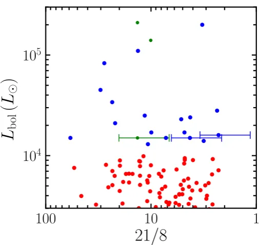
Fig. 1.Sample selection plot where the luminosity (in units of L) is

plotted against the MSX 21/8µm color. Horizontal bars mark uncer-tainties in the color. While the blue sources fulfill our selection criteria, the red ones are below our luminosity cut of 104_{L. Green sources are} those for which high-resolution mm data already exist and which were therefore excluded from the observations.

high-mass star-forming regions NGC 7538IRS1 and NGC 7538S revealed that NGC 7538S has fragmented into several subsources at∼0.300 resolution whereas at the same spatial resolution the central core of NGC 7538IRS1 remains a single compact source (Beuther et al. 2012; see alsoQiu et al. 2011for more extended cores in the environment). At an even higher angular resolu-tion of ≤0.200 _{or spatial scales below 1000 AU, Beuther et al.} (2013) found that even the innermost structure of NGC 7538IRS1 starts to fragment. This implies that the scales of fragmenta-tion do vary from region to region. Other fragmentafragmenta-tion studies do not entirely agree on the physical processes responsible for driving the fragmentation. For example, the infrared dark cloud study by Wang et al. (2014) indicates that turbulence may be needed to explain the large fragment masses. Similarly,

Pillai et al.(2011) argue for two young pre-protocluster regions that turbulent Jeans fragmentation can explain their data. How-ever, other studies like those byPalau et al.(2013,2014,2015) favor pure gravitational fragmentation. Similar results are also indicated in a recent ALMA study toward a number of hyper-compact HII regions (Klaassen et al. 2018). In addition to the thermal and turbulent gas properties, theoretical as well as observational investigations indicate the importance of the mag-netic field for the fragmentation processes during (high-mass) star formation (Commerçon et al. 2011;Peters et al. 2011; Tan et al. 2013; Fontani et al. 2016). Furthermore, radiation feed-back from forming protostars is also capable of reducing the fragmentation of the high-mass star-forming region (e.g.,

Krumholz et al. 2007).

−120 −60 0 60 120 Off set ( ′′) IRAS23151

0.25 pc

IRAS23033

0.25 pc

AFGL2591

0.25 pc

G075.78

0.25 pc

S87 IRS1

0.25 pc

−120 −60 0 60 120 Off set ( ′′) S106

0.25 pc

IRAS21078

0.25 pc

G100.38

0.25 pc

G084.9505

0.25 pc

G094.6028

0.25 pc

−120 −60 0 60 120 Off set ( ′′) CepA HW2

0.25 pc

NGC7538 IRS9

0.25 pc

W3 H2O

0.25 pc

W3 IRS4

0.25 pc

G108.75

0.25 pc

−120 −60 0 60 120

Offset (′′)

−120 −60 0 60 120 Off set ( ′′) IRAS23385

0.25 pc

−120 −60 0 60 120

Offset (′′)

G138.2957

0.25 pc

−120 −60 0 60 120

Offset (′′)

G139.9091

0.25 pc

−120 −60 0 60 120

Offset (′′)

NGC7538 IRS1

0.25 pc

−120 −60 0 60 120

Offset (′′)

NGC7538 S

0.25 pc

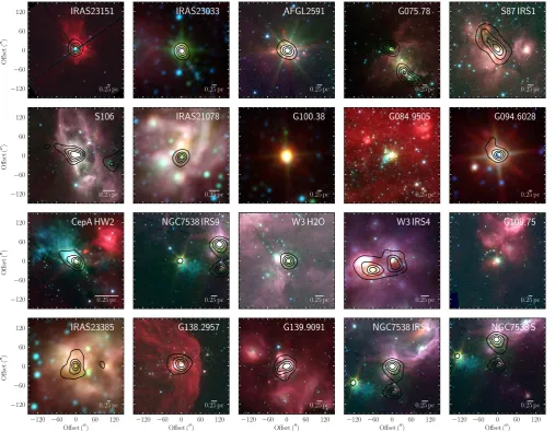
Fig. 2.Large-scale overview images for the whole CORE sample. The color scale shows three-color images with blue, green, and red fromSpitzer

3.6, 4.5, and 8.0µm for all sources except IRAS 23033, IRAS21078, G100, G094, and IRAS 23385 for which WISE 3.4, 4.6, and 12µm data are presented. Furthermore, W3IRS4 usesSpitzer3.6, 4.5µm, and MSX 8µm. The contours show SCUBA 850µm continuum data (di Francesco et al. 2007; contour levels 20%, 40%, 60%, and 80% of the peak emission) for all sources except G100, G084, and G108 where these data do not exist.

of pc-scale clumps into cores with sizes of typically several thousand AU. Smaller-scale disk fragmentation will also be addressed by the CORE program (see Sect. 3) through the spectral line analysis of high-mass accretion disk candidates (e.g.,Ahmadi et al. 2018).

The previous investigations of NGC 7538IRS1 and

NGC 7538S (Beuther et al. 2012, 2013; Feng et al. 2016) can be considered as a pilot study for the CORE survey presented here. With an overall sample of 20 high-mass star-forming regions (see sample selection below) observed at uniform angular resolution (∼0.300−0.400) in the 1.3 mm wave-length band with NOEMA, we can investigate how (un)typical such fragmentation properties on core scales are. Fragmentation signatures to be investigated are, for example, the fragment mass, size and separation distributions, and how they relate to basic underlying physical processes.

In this paper, we present the sample selection, the general survey strategy as well as the observational characteristics. The remaining of the paper focuses on the continuum data and frag-mentation properties of the sample. The other scientific aspects of this survey will be presented in separate publications (e.g.,

Ahmadi et al. 2018; Mottram et al. in prep.; Bosco et al. in prep.).

2. Sample

Our sample of young high-mass star-forming regions was selected to fulfill several criteria. (a) Regions of our sample have luminosities>104_L

indicating that at least an 8Mstar is forming. (b) Distances are limited to below 6 kpc to ensure high linear resolution (∼1000 AU). (c) The sources are high-declination (decl.>24◦) to obtain the best possibleuv-coverage (implying that they are either not at all or at most poorly accessible with the Atacama Large Millimeter Array, ALMA). Furthermore, only sources with extensive complementary high-spatial resolution observations at other wavelengths were selected to better characterize their overall properties. In this context, the sample is also part of a large e-Merlin project led by Co-I Melvin Hoare to characterize the cm continuum emission of the sample at an anticipated spatial resolution of down to 30 mas. The initial luminosity selection was based on luminosity and color–color criteria. Figure 1 presents the corresponding luminosity–color plot. We used the luminosity-color plot as a sample selection tool as the y- and x-axes act as proxies for stellar mass and evolutionary stage, respectively. By the time massive forming stars have reached 104_L

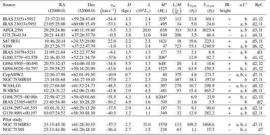
Table 1.CORE sample (grouped in track-sharing pairs).

Source RA Dec 3lsr D L Ma L/M S8µm S21µm IR- a.f.e Ref.

(J2000.0) (J2000.0) km s−1

(kpc) (104_L

) (M)

L

M

(Jy) (Jy) bright

IRAS 23151+5912 23:17:21.01 +59:28:47.49 –54.4 3.3 2.4 215b _{112 23.8 101.1 + b d1, l2}

IRAS 23033+5951 23:05:25.00 +60:08:15.49 –53.1 4.3 1.7 495 34 5.0 24.0 – a, b d2, l1

AFGL2591 20:29:24.86 +40:11:19.40 –5.5 3.3 20.0 638 313 313.8 1023.4 + a, b d3, l1

G75.78+0.34 20:21:44.03 +37:26:37.70 –0.5 3.8 11.0 549 200 3.5 46.4 – a, c d4, l1

S87 IRS1 19:46:20.14 +24:35:29.00 22.0 2.2 2.5 1421 18 19.6 225.1 + a d5, l1

S106 20:27:26.77 +37:22:47.70 –1.0 1.3 3.4 47 723 53.1 1240.9 + a, b d6, l2

IRAS 21078+5211 21:09:21.64 +52:22:37.50 –6.1 1.5 1.3 177 73 2.1 8.8 – a, b dl1

G100.3779−03.578 22:16:10.35 +52:21:34.70 –37.6 3.5 1.5 206d _{12.9 92.7 + b d1, l2}

G084.9505−00.691 20:55:32.47 +44:06:10.10 –34.6 5.5 1.3 648c _{20 1.4 14.6 + b d2, l2}

G094.6028−01.797 21:39:58.25 +50:14:20.90 –43.6 4.0 2.8 1525 18 63.9 150.5 + b, c d1, l2

CepAHW2 22:56:17.98 +62:01:49.50 –10.0 0.7 1.5 40 375 4.6 271.7 – a, b, c d7, l1

NGC 7538IRS9 23:14:01.68 +61:27:19.10 –57.0 2.7 2.3 214 107 38.1 197.0 + b d7, l1

W3(H2O) 02:27:04.60 +61:52:24.73 –48.5 2.0 8.3 307 270 10.7 298.9 – a, b, c d8, l2

W3IRS4 02:25:31.22 +62:06:21.00 –42.8 2.0 4.5 481 93 15.4 465.2 + a, b d8, l1

G108.7575−00.986 22:58:47.25 +58:45:01.60 –51.5 4.3 1.4 6204d _{6.9 21.9 + b, c d2, l3}

IRAS 23385+6053 23:40:54.40 +61:10:28.20 –50.2 4.9 1.6 510 31 1.6 3.5 – b dl2

G138.2957+01.555 03:01:31.32 +60:29:13.20 –37.5 2.9 1.4 197 71 9.1 90.0 + a, b d2, l1

G139.9091+00.197 03:07:24.52 +58:30:48.30 –40.5 3.2 1.1 349 32 12.9 282.2 + a, b d2, l1

Pilot study

NGC 7538IRS1 23:13:45.36 +61:28:10.55 –57.3 2.7 21.0 1570 133 109.2 1468.6 + a, b, c d7, l1

NGC 7538S 23:13:44.86 +61:26:48.10 –56.4 2.7 1.5 238 63 1.1 15.3 – b, c d7

Notes.(a)_{Masses are calculated mainly from the SCUBA 850µm fluxes byDi Francesco et al.(2008).}(b)_{Based on 1.2 mm continuum data from}

Beuther et al.(2002).(c)_{Based on 1.1 mm continuum data fromGinsburg et al.(2013).}(d)_{Based on C}18_{O(3–2) data fromMaud et al.(2015); effective} radii for G100∼0.34 pc and for G108∼1.4 pc.(e)_{Associated features (a.f.), a: cm continuum; b: H}

2O maser; c: CH3OH maser.

References.d1:Choi et al. 1993, d2:Urquhart et al. 2011, d3:Rygl et al. 2012, d4:Ando et al. 2011, d5:Xu et al. 2009, d6: Xu et al. 2013, d7:Moscadelli et al. 2009, d8:Hachisuka et al. 2006;Xu et al. 2006, dl1:Molinari et al. 1996, dl2:Molinari et al. 1998, l1: RMS survey database (http://rms.leeds.ac.uk/cgi-bin/public/RMS_DATABASE.cgi), using SED fitting fromMottram et al.(2011) includingHerschelfluxes and the latest distance determination, l2: RMS survey database (http://rms.leeds.ac.uk/cgi-bin/public/RMS_DATABASE.cgi), using SED fitting fromMottram et al.(2011) updated to the latest distance determination, l3: RMS survey database (http://rms.leeds.ac.uk/ cgi-bin/public/RMS_DATABASE.cgi), calculated from the MSX 21µm flux using the scaling relation derived byMottram et al.(2011) and updated to the latest distance determination.

determined primarily by the stellar mass as at this stage the accretion luminosity only contributes a small fraction of the total luminosity even at high-accretion rates (e.g.,Hosokawa & Omukai 2009; Hosokawa et al. 2010; Kuiper & Yorke 2013;

Klassen et al. 2016). We also expect that over time the IR colors will evolve from red to blue as the envelope material is dispersed and/or accreted (e.g.,Zhang et al. 2014).

Many sample sources are covered by the Red MSX sources survey (RMS;Lumsden et al. 2013), and a few additional promi-nent northern hemisphere regions are included as well. Our sample excludes the few sources that fulfill these selection cri-teria but which already have been observed at mm wavelengths with high angular resolution (e.g., W3IRS5, NGC 7538IRS1/S;

Rodón et al. 2008; Beuther et al. 2012). The resulting sam-ple of 18 regions is comsam-plete within these described selection criteria. Because NGC 7538IRS1 and NGC 7538S were observed in an almost identical setup (only the compact D-array data were not taken), they are considered as a pilot study and their results are incorporated into the analysis of the CORE project. Table1

presents a summary of the main source characteristics, including their local-standard-of-rest velocity 3lsr, distance D, luminos-ity L, mass M (see also Sect. 5.3), their 8 and 21µm fluxes, H2O, CH3OH maser and cm continuum associations as well as references for the distances and luminosities. Figure2 shows a larger-scale overview of the twenty regions with the near- to mid-infrared data shown in color and the 850µm continuum

single-dish data (Di Francesco et al. 2008) presented in contours.

Regarding the evolutionary stage of the sample, they are all luminous and massive young stellar objects (MYSOs) or otherwise named high-mass protostellar objects (HMPOs). Subdividing the regions a bit further, some regions show very strong (sub)mm spectral line emission indicative of hot molec-ular cores (AFGL2591, G75.78+0.34, CepAHW2, W3(H2O), NGC 7538IRS1), other regions are line-poor (e.g., S87IRS1,

S106, G100.3779, G084.9505, G094.6028, G138.2957,

G139.9091), and the remaining sources exhibit intermediate-rich spectral line data. Furthermore, the sample covers various com-binations of associated cm continuum, H2O and class II CH3OH maser emission (Table 1). Following Motte et al. (2007), we checked whether the sources belong to the so-called IR-bright or IR-quiet categories with the dividing line defined as IR-quiet

whenS21µm<10 Jy

_{1.7 kpc}

D

2 _L

1000L

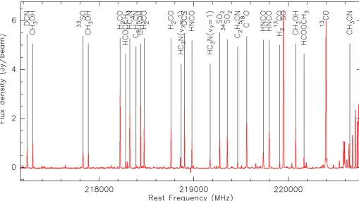
Fig. 3.Example wide-band spectrum extracted toward AFGL2591. The most important lines in the bandpass are marked.

embedded stage, they are already capable of driving dynamic outflows, have high luminosities, and produce a rich chemistry.

A different evolutionary time indicator sometimes used is the luminosity-over-mass ratioL/Mof the regions (see Table1; e.g.,Sridharan et al. 2002;Molinari et al. 2008,2016;Ma et al. 2013;Cesaroni et al. 2017;Motte et al. 2018). The CORE sample covers a relatively broad range in this parameter space between roughly 20 and 700L/M. However, this ratio is not entirely conclusive either. For example, the region with our lowest ratio (S87IRS1 with L/M ∼18L/M), that could be indicative of relative youth, is classified otherwise as IR-bright which seems counterintuitive at first sight. Since the various age-indicators are derived from parameters averaged over different scales, it is possible that they are averaging over subregions with varying evolutionary stages and are hence not giving an unambiguous evolutionary picture.

In summary, the CORE sample consists of regions contain-ing HMPOs/MYSOs above 104L from the pre-hot-core stage to typical hot-cores and also a few more evolved regions that have likely already started to disrupt their original gas core. The evolutionary stages are comparable to the sample byPalau et al.

(2013,2015) with the difference that they had a large fraction of sources below 104Land even below 103L(only four regions above 104_L

).

3. CORE large program strategy

Following our experience with NGC 7538IRS1 and NGC 7538S (Beuther et al. 2012, 2013), we devised the CORE survey in a similar fashion. The full sample is observed in the 1.3 mm band, and a subsample of five regions will also subsequently be observed at 843µm. Here we focus on the 1.3 mm part of the

survey for the full sample. The shorter wavelength study will be presented once it is complete.

Several aspects were considered to achieve the goals of the project: (i) the most extended A-configuration of NOEMA was used for the highest possible spatial resolution. (ii) Com-plementary observations with more compact configurations of the interferometer recover information on larger spatial scales. Simulations showed that adding the B and D configurations provided the best compromise between spatial information and observing time. (iii) To also cover very extended spectral line emission, short spacing observations from the IRAM 30 m tele-scope were added. (iv) Spectrally, among other lines our survey covers CH3CN to trace high-density gas as might be found in accretion disks and/or toroids (e.g., Cesaroni et al. 2007) and H2CO which traces lower-density, larger-scale structures. Both, CH3CN and H2CO are also well known temperature trac-ers (e.g.,Mangum & Wootten 1993; Zhang et al. 1998;Araya et al. 2005). Furthermore, outflow tracers such as 13CO and SO are included. A plethora of additional lines are also cov-ered to investigate the chemical properties of the regions. An early example of such investigation can be found in the paper about the pilot study sources NGC 7538IRS1 and NGC 7538S by

Feng et al.(2016).

Table 2.Spectral lines at high spectral resolution.

Line ν Eu/k

(GHz) (K)

H2CO(30,3−20,1) 218.222 21

HCOOCH3(173,14−163,13) 218.298 100

HC3N(24−23) 218.325 131

CH3OH(42,2−31,2) 218.440 46

NH2CHO(101,9−91,8) 218.460 61

H2CO(32,2−22,1) 218.476 68

OCS(18−17) 218.903 100

HCOOCH3(174,13−164,12) 220.167 103 CH2CO(111,11−101,10) 220.178 77 HCOOCH3(174,13−164,12) 220.190 103

CH3CN(126−116) 220.594 326

CH13₃ CN(123−113) 220.600 133

CH13

3 CN(122−112) 220.621 98

CH3CN(125−115) 220.641 248

CH3CN(124−114) 220.679 183

CH3CN(123−113) 220.709 133

CH3CN(122−112) 220.730 98

CH3CN(121−111) 220.743 76

CH3CN(120−110) 220.747 69

band correlator units to specific spectral locations that covered the most important lines at a spectral resolution of 0.312 MHz, corresponding to a velocity resolution of ∼0.43 km s−1 _{at the} given frequencies. Table 2 shows the spectral lines covered at this high-spectral resolution. For more details about the spectral line coverage we refer the reader to the CORE paper byAhmadi et al.(2018).

For the complementary IRAM 30 m short spacings observa-tions, we mapped all regions with approximate map sizes of 10 in the on-the-fly mode in the 1 mm band. Since the bandpasses at the 30 m telescope are broader and the receivers work in a double-sideband mode, the 30 m data cover a broader range of frequencies between∼213 and∼221 GHz in the lower sideband and between ∼229 and∼236 GHz in the upper sideband. The line data that are covered by the NOEMA and 30 m observations can be merged and imaged together, whereas the remaining 30 m bandpass data can be used as standalone data products. Since we did not use the single-dish data for the continuum study pre-sented here, we refer to the CORE paper by Mottram et al. (in prep.) for more details on the IRAM 30 m data.

More details about the CORE project are provided at the team web-page1_{. There, we will also provide the final calibrated}

visibility data and imaged maps. The data release will take place in a staged fashion. The continuum data are published here, and the corresponding line data will be provided with subsequent publications.

4. Observations

The entire CORE sample (except the pilot sources

NGC 7538IRS1 and NGC 7538S) was observed at 1.37 mm between summer 2014 and January 2017 in the three PdBI/NOEMA configurations A, B and D to cover as many spatial scales as possible (see Sect. 3). The baseline ranges for all tracks in terms of uv-radius are given in Table 3. The

1 _{http://www.mpia.de/core}

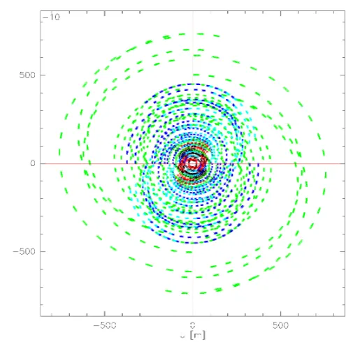
Fig. 4.Exampleuv-coverage for CepA. The different colors correspond

to different observed (half-)tracks. Red and black correspond to D-array observations, blue and cyan to B-array, and green to A-array data.

shortest baselines, typically between 15 and 20 m, correspond to theoretically largest recoverable scales of 1600−2000. For each track, two sources were observed together in a track-sharing mode. The phase centers of each source and the respective source pairs for the track-sharing are shown in Table 1. Since each source was observed in three different configurations, at least three (half-) tracks were observed per source. Depending on the conditions, several source pairs were observed in more than three (partial) tracks in order to achieve the required sensitivity anduv-coverage. Altogether, this multi-configuration and multi-track approach resulted in excellent uv-coverage for each source, an example of which is shown in Fig.4. Typically two phase calibrators were observed in the loops with the track-sharing pairs. For the final phase calibration, we mostly used only the stronger ones. Depending on array configuration and weather conditions, the phase noise varied between∼10 and

∼50 deg. Bandpass calibration was conducted with observations of strong quasars, for example, 3C84, 3C273, or 3C454.3. The resulting spectral baselines are very good, over the broad WIDEX bandpass as well as the narrow-band bandpasses (e.g., see Fig.3). The absolute flux calibration was conducted in most cases with the source MWC349 where an absolute model flux of 1.86 Jy at 220 GHz was assumed2_{. For only very few tracks}

in which that source was not observed, the flux calibration was conducted with other well-known calibrators (e.g., LKHα101). The absolute flux scale is estimated to be correct to within 20%. To achieve the highest angular resolution, uniform weighting was applied during the imaging process. The final synthesized beams for the continuum combining all NOEMA data vary between ∼0.3200 _and∼0.500 _{with exact values for each source} given in Table 3. The full width at half maximum of the primary beam of our observations is ∼2200. To create the con-tinuum images, we carefully inspected the WIDEX bandpasses for each source individually and created the continuum from

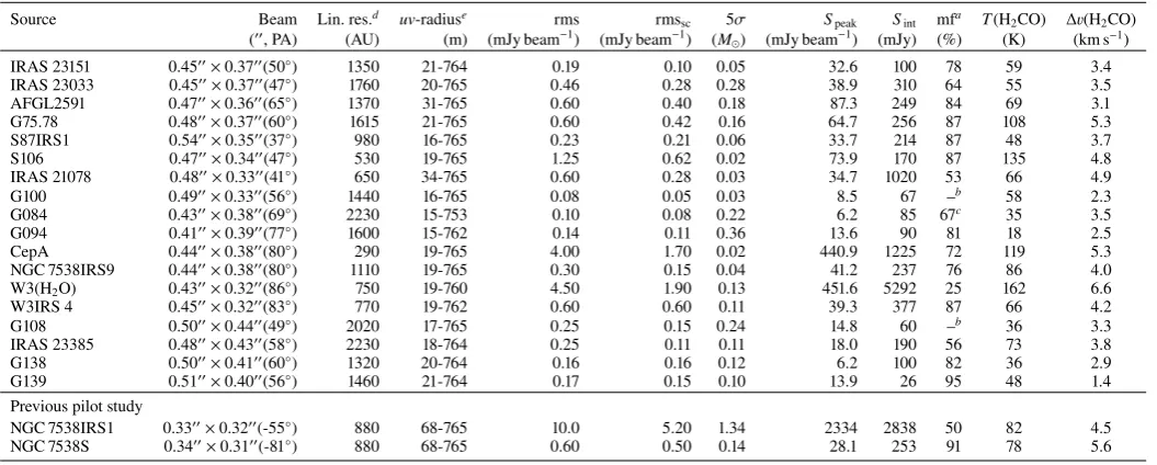
Table 3.CORE parameters.

Source Beam Lin. res.d _uv-radiuse _{rms rms}

sc 5σ Speak Sint mfa T(H2CO) ∆3(H2CO)

(00_{, PA) (AU) (m) (mJy beam}−1_{) (mJy beam}−1_{) (M}

) (mJy beam−1) (mJy) (%) (K) (km s−1)

IRAS 23151 0.4500_×0.3700₍₅₀◦_{) 1350 21-764 0.19 0.10 0.05 32.6 100 78 59 3.4}

IRAS 23033 0.4500_×0.3700₍₄₇◦_{) 1760 20-765 0.46 0.28 0.28 38.9 310 64 55 3.5}

AFGL2591 0.4700_×0.3600₍₆₅◦_{) 1370 31-765 0.60 0.40 0.18 87.3 249 84 69 3.1}

G75.78 0.4800_×0.3700₍₆₀◦_{) 1615 21-765 0.60 0.42 0.16 64.7 256 87 108 5.3}

S87IRS1 0.5400_×0.3500₍₃₇◦_{) 980 16-765 0.23 0.21 0.06 33.7 214 87 48 3.7}

S106 0.4700_×0.3400₍₄₇◦_{) 530 19-765 1.25 0.62 0.02 73.9 170 87 135 4.8}

IRAS 21078 0.4800_×0.3300₍₄₁◦_{) 650 34-765 0.60 0.28 0.03 34.7 1020 53 66 4.9}

G100 0.4900_×0.3300₍₅₆◦_{) 1440 16-765 0.08 0.05 0.03 8.5 67 –}b _{58 2.3}

G084 0.4300_×0.3800₍₆₉◦_{) 2230 15-753 0.10 0.08 0.22 6.2 85 67}c _{35 3.5}

G094 0.4100_×0.3900₍₇₇◦_{) 1600 15-762 0.14 0.11 0.36 13.6 90 81 18 2.5}

CepA 0.4400_×0.3800₍₈₀◦_{) 290 19-765 4.00 1.70 0.02 440.9 1225 72 119 5.3}

NGC 7538IRS9 0.4400_×0.3800₍₈₀◦_{) 1110 19-765 0.30 0.15 0.04 41.2 237 76 86 4.0}

W3(H2O) 0.4300×0.3200(86◦) 750 19-760 4.50 1.90 0.13 451.6 5292 25 162 6.6

W3IRS 4 0.4500_×0.3200₍₈₃◦_{) 770 19-762 0.60 0.60 0.11 39.3 377 87 66 4.2}

G108 0.5000_×0.4400₍₄₉◦_{) 2020 17-765 0.25 0.15 0.24 14.8 60 –}b _{36 3.3}

IRAS 23385 0.4800_×0.4300₍₅₈◦_{) 2230 18-764 0.25 0.11 0.11 18.0 190 56 73 3.8}

G138 0.5000_×0.4100₍₆₀◦_{) 1320 20-764 0.16 0.16 0.12 6.2 100 82 36 2.9}

G139 0.5100_×0.4000₍₅₆◦_{) 1460 21-764 0.17 0.15 0.10 13.9 26 95 48 1.4}

Previous pilot study

NGC 7538IRS1 0.3300_×0.3200_(-55◦_{) 880 68-765 10.0 5.20 1.34 2334 2838 50 82 4.5}

NGC 7538S 0.3400_×0.3100_(-81◦_{) 880 68-765 0.60 0.50 0.14 28.1 253 91 78 5.6}

Notes.The columns give the synthesized beam, the linear resolution, the baseline range (uv-radius), the rms noise before and after self-calibration, the 5σ mass sensitivity, the measured peak, and integrated flux densitiesSpeak andSint, the missing flux ratios as well as the H2CO derived temperaturesT and line widths∆3.(a)_{Missing flux, for details see main text,}(b)_{no single-dish data available,}(c)_{based on BOLOCAM 1.1 mm flux} measurement in 4000

aperture (Ginsburg et al. 2013),(d)_{average linear resolution,}(e)_{projected uv baseline range.}

the line-free parts only. The 1σcontinuum rms correspondingly varies from source to source. This depends not only on the cho-sen line-free channels, but also on the side-lobe noise introduced by the strongest sources in the fields. Although theuv-coverage is very good (Fig.4), not all side-lobes can be properly subtracted, and the final noise also depends on theuv-coverage.

To reduce calibration, side-lobe and imaging issues, we explored how much self-calibration would improve the data qual-ity. For that purpose, we exported the continuum uv-tables to CASA format and did the self-calibration within CASA (ver-sion 4.7.2; McMullin et al. 2007). We performed phase self-calibration only, and the time intervals used for the process varied from source to source depending on the source strength. Solution intervals of either 220, 100, or 45 s were used, where 45 s is the smallest possible interval due to averaging of the data during data recording. Interactive masking during the self-calibration loops was applied, with only the strong peaks used in the first iterations and then subsequently adapted to the weaker structures. After the self-calibration, we again exported the data toGILDASformat and conducted all the imaging withinGILDAS to enable direct comparisons with the original datasets. Again, uniform weighting was applied and we cleaned the data down to a 2σthreshold. To show the differences of the images prior to and after the self-calibration process, Appendix Cpresents the derived images before and after the self-calibration. The contour-ing is done in both cases in 5σsteps. Careful inspection of all data shows that no general structural changes were created dur-ing the self-calibration process. The self-calibration improved the data considerably with reduced rms noise and slightly increased peak fluxes. We find that the flux-ratios between the main substructures within individual regions remained rel-atively constant prior to and after self-calibration. Below, we conduct the analysis with the self-calibrated dataset. Table 3

presents the 1σcontinuum rms for all sources before and after self-calibration. We typically achieve sub-mJy rms with a range between 0.05 and 1.9 mJy beam−1 for the 18 new targets. Only

the pilot source NGC 7538IRS1 has a slightly higher rms of 5.2 mJy beam−1 which can be attributed to the higher source strength and the missing D-array observations. Primary-beam correction was applied to the final images, and the fluxes were extracted from these primary-beam corrected data (Sect. 5.2). Evaluating the measured peak flux densitiesSpeakand noise val-ues (rmssc) in Table3, we find S/N of between 39 and 326 with the majority of region (13) exhibiting S/N greater than 100. We provide the original pre-self-calibration images, the images after applying self-calibration as well as the primary-beam corrected images in electronic form3.

Simulated observations. To better understand how the

imag-ing affects our results, we simulated a typical observation. The details of the simulations can be found in AppendixB. In the following, we summarize the method and results. We used real single-dish dust continuum data from the large-scale SCUBA-2 850µm map of Orion byLane et al.(2016), converted the flux to 1.37 mm wavelength (assuming a ν3.5 _{frequency-relation),} rescaled the spatial resolution and flux density to a distance of 3 kpc, and imaged different parts of Orion with the typical uv-coverage and integration time from the CORE project. Sim-ilar to our observations, the rms varied depending on whether a strong source (in this case Orion-KL) was present in the observed field. While the point source mass sensitivity is very good, between 0.01 and 0.1M (depending on the rms), with our spatial resolution typical Orion cores are extended struc-tures, rather than point sources, even at a distance of 3 kpc. Hence, the dependence of the rms noise on the strongest sources in the field strongly affects the actual core mass sensitivity for extended structures as well. Taking the two examples shown in AppendixB, cores with masses down to∼1Mare detectable in fields without very strong sources. If such a low-mass core were within the stronger Orion-KL field, it would not be detectable

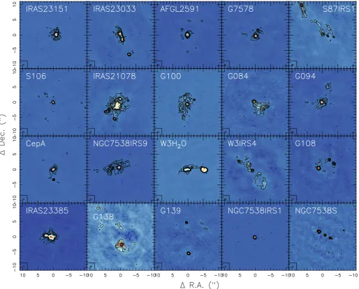
Fig. 5.Compilation of 1.37 mm continuum images for CORE sample on the same angular scale. The contouring is in 5σsteps (see Table3). The sources are labeled in each panel, and the synthesized beams are shown at the bottom-left of each panel. A comparison figure converted to linear scales is shown in Fig.6. Magnifications and absolute flux-scales are shown in AppendixC.

anymore. Therefore, the core mass sensitivities strongly depend on the strongest and most massive sources within the respective observed fields. The dynamic range limit of the simulations of Orion-KL is approximately 53.

5. Continuum structure and fragmentation results 5.1. Source structures

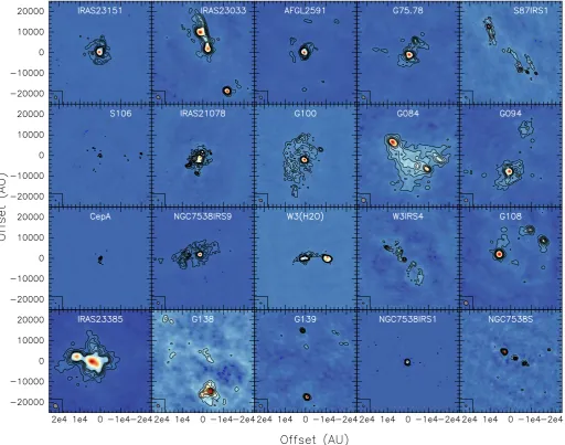
Figures5and6present the 1.37 mm continuum data of the full CORE sample. While Fig.5 shows the data in angular resolu-tion over the full area of the primary beam of the observaresolu-tions, Fig. 6uses the distances of the sources (Table 1) and presents the data at the same linear scales, making direct comparisons between sources possible. The first impression one gets from these dust continuum images is that the structures are far from uniform. While some sources are dominated by single cores (e.g., IRAS 23151, AFGL2591, S106, NGC 7538IRS1), other regions clearly contain multiple cores with a lot of substructures (e.g., S87IRS1, IRAS 21078, W3IRS4), some of which have more than ten cores within a single observed field (see Sect.5.2).

We see no correlation between the number of fragments and the distances to the sources. We discuss this fragmentation diversity in more detail in Sect.6.

5.2. Source extraction

To extract the sources from our 20 images, we used the clas-sical CLUMPFIND algorithm by Williams et al. (1994) on our self-calibrated images. As input parameters we used the 5σ con-tour levels presented in Figs.5and6as well as in AppendixC. These images sometimes also show negative 5σcontours, indi-cating that the interferometric noise is neither uniform nor really Gaussian. Therefore, we inspected all sources identified byCLUMPFINDindividually and only included those where the peak flux density is ≥10σ (two positive contours minimum in AppendixC). The derived positional offsets from the phase cen-ter, peak flux densities Speak, integrated flux densitiesSint and equivalent core radii (calculated from the measured core area assuming a spherical distribution) are presented in Table A.1

Fig. 6.Compilation of 1.37 mm continuum images for CORE sample converted to linear resolution elements. The contouring is in 5σsteps (see Table3). The sources are labeled in each panel, and the synthesized beams are shown at the bottom-left of each panel.

To estimate the amount of missing flux filtered out by the interferometric observations, we extracted the 850µm peak flux densities from single-dish observations, mainly from the SCUBA legacy archive catalog (Di Francesco et al. 2008). Since this dataset has a final beam size of 22.900it covers our primary beam size very well. Scaling this 850µm data with a typical ν3.5 _{dependency to the approximate flux at our observing} fre-quency of 220 GHz, we can compare these values to the sum of the integrated fluxes measured for each target region from our previousCLUMPFINDanalysis. Table3presents the correspond-ing misscorrespond-ing flux values (mf in percentage) for the sample (for two regions – G100 & G108 – we did not find corresponding single-dish data). The amount of missing flux varies signifi-cantly over the sample, typically ranging between 60 and 90%. The only extreme exception is W3(H2O) where only 25% of the flux is filtered out. This implies that for this region the flux is strongly centrally concentrated without much of a more extended envelope structure. For the remaining sources, even with the comparably good uv-coverage (Fig. 4) a significant fraction of the flux is filtered out. The variations from source to source indicate that the spatial density structure also varies strongly from region to region (see discussion in Sect.6).

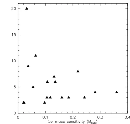
There is a broad distribution in the number of cores identi-fied in each region. We find between 1 and 20 cores among the different regions (see Table4). To check whether this range of identified cores is related to our mass sensitivity, in Fig.7we plot the 5σmass sensitivity (Table3and Sect.5.3) vs. the number of identified cores (excluding NGC 7538IRS1 because of its unusu-ally poor mass sensitivity limit, Table3). While there might be a slight trend of more cores toward lower mass sensitivity limits, our lowest mass sensitivity limit region CepA also shows only two cores. In the main regime of 5σmass sensitivities between 0.1 and 0.3Mwe do not see a relation between the number of identified cores and the mass sensitivity. Hence, the number of identified cores does not seem to be strongly dependent on our mass sensitivity limits below 0.4M.

5.3. Mass and column density distributions

Assuming optically thin dust continuum emission at 220 GHz, we can estimate the gas masses and peak column densities for all identified cores in the sample. Following the original outline by Hildebrand (1983) in the form presented by Schuller et al.

Fig. 7.Number of identified cores plotted against the 5σmass sensi-tivity. NGC 7538IRS1 is excluded because of its unusually high mass sensitivity limit.

dust mass absorption coefficientκof 0.9 cm2_g−1_{(Ossenkopf &}

Henning 1994at densities of 106_cm−3_{with thin ice mantles) and} average temperatures for each region derived from the CORE IRAM 30 m H2CO data. H2CO is a well-known gas thermometer in the ISM (Mangum & Wootten 1993), and we derive beam-averaged temperatures from the single-dish spectra toward the peak positions of each region at a spatial resolution of 1100. For the temperature estimates we fitted the data with the XCLASS tool (eXtendedCASALine Analysis Software Suite) tool (Möller et al. 2017). XCLASS models the spectra by solving the radia-tive transfer equation for an isothermal homogeneous object in local thermodynamic equilibrium (LTE), using the molecular databases VAMDC and CDMS4 _{(Müller et al. 2001). XCLASS}

employs the model optimizer package MAGIX (Modeling and Analysis Generic Interface for eXternal numerical codes) to find the best fit solutions (Möller et al. 2013). The derived temper-atures are shown in Table 3. Since we derive beam-averaged temperatures from the single-dish data, the actual temperatures of individual cores at smaller spatial scales may vary compared to those beam-averaged temperatures. More detailed tempera-ture analysis from the combined interferometer plus single-dish data is beyond the scope of this paper and will be conducted in future work on the CORE data. The mass estimates are in general lower limits since we are filtering out large-scale flux that may be associated with the dense cores (see also AppendixB). Furthermore, while the optically thin assumption for the dust emission should be valid in most cases, there may be some exceptions like CepA where high peak flux densities (Tables3andA.1) imply high brightness temperatures indicat-ing moderate optical depth at these peak positions. However, since the masses are calculated typically over areas larger than just the peak, and the brightness temperatures decrease quickly with distance from the peak, this effect should be comparably weak.

The derived core masses and column densities are presented in Table A.1 and roughly span 0.1 to 40M, and 5×1022

4 _{http://www.vamdc.org}

to 1025cm−2. For the mass and column density analysis, we excluded sources for which the continuum emission is clearly dominated by HIIregions and hence show barely dust contin-uum emission. These are specifically W3(OH) (cores #1 and #2 in W3(H2O), the southern ring-like region in W3IRS4 (sources #5 and #6) and core #2 in S87IRS1. For several other cores, the fluxes were corrected for free–free emission for the mass determinations (see TableA.1).

Using similar assumptions, we also re-estimated the large-scale mass reservoir for the sample. For most sources, we used the integrated 850µm fluxes derived by Di Francesco et al.

(2008), while for IRAS 23151 the 1.2 mm flux was derived from the MAMBO data presented in Beuther et al. (2002), and for

G084 we used the 1.1 mm BOLOCAM data from Ginsburg

et al.(2013). The used gas-to-dust mass ratio and average H2CO derived temperatures are the same as above, and we used for the single-dish data dust absorption coefficients κof 0.78, 0.9, and 1.4 cm2_g−1 _{at 1.2, 1.1, and 0.85 mm wavelengths,} respec-tively (Ossenkopf & Henning 1994; at densities of 105cm−3). The derived total masses are presented in Table1(for G100 and G108, the masses are taken from C18O(3–2) data from Maud et al. 2015). While the regions have typical mass reservoirs of several 100M, the sample spans a comparably broad range between∼40 and∼1500M(for G108 even higher masses are measured, however over a comparably large area with radius 1.4 pc, Table1andMaud et al. 2015).

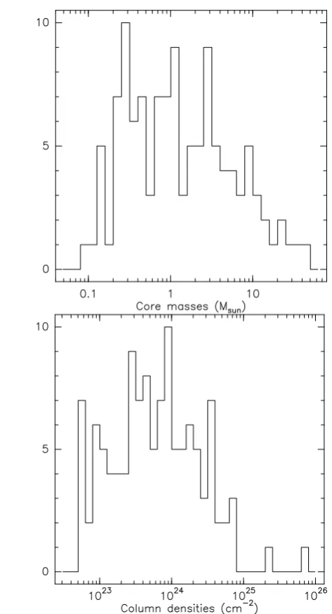
For the NOEMA-only derived core parameters, Fig.8shows histograms of the masses and column densities. The combined mass distribution shows that most detected cores are in the range between∼0.1 and∼10Mwith only a few cores exceed-ing 10M. The most massive core is in NGC 7538IRS1 with 43M(although significant free-free contamination may affect the estimate for this source,Beuther et al. 2012). Regarding the cores in excess of 10M, there is no clear trend whether they are found as isolated objects or embedded in fragmented regions. For example, comparably massive cores are found in the low-fragmentation regions NGC 7538IRS1 or AFGL2591, but cores of similar mass are also found in more fragmented regions like IRAS 23151, IRAS 23033, G75.78, as well as in the intermedi-ately fragmented region W3(H2O). The peak column densities are very large, typically exceeding 1023_cm−2 _{and even going} above 1025cm−2 for a few exceptional regions. Figure9 plots the column densities against the masses, and while we see a scatter, there remains nevertheless a trend that column densities and masses are correlated. If one takes into account the distance-dependencies of our derived parameters (color-coding in Fig.9), we see that the higher-mass-lower-column-density sources are found at on average larger distances. With increasing distance, the physical size of the beam (where the column density is measured within), increases as well. Such larger area beams cover the central highest-column-density peak position but also more lower-column-density environmental gas. This smoothing slightly decreases the measured column densities with increas-ing distance. The other way round, increasincreas-ing the covered area with distance also increases the measured masses. Hence, part of the scatter in Fig. 9 is caused by the distance range of our sample. For smaller distance bins, the scatter is significantly reduced.

Fig. 8.Histograms of masses (top panel) and column densities (bottom panel) for all detected cores.

108_cm−3_{, there is no clear trend between the densities and the} masses. Taking the distances into account again, the scatter is reduced but identifying trends within distance-limited ranges is still difficult. Hence, in this sample, the core densities are sim-ilar over the whole range of observed core masses. Having a correlation between mass and column density but less good cor-relation between mass and average density implies that the core masses should correlate with their sizes (their equivalent radii). Figure 11 presents the corresponding data again color-coded with distance. And indeed mass and size are well correlated for the sample, again much tighter if one looks at limited distance ranges. Figure 11also plots lines of constant column densities between 1023and 1025cm−2. While most regions scatter between the 1023 and 1024cm−2 lines, also subsamples between limited distance ranges do not follow constant column density distribu-tions but increase in column density with increasing mass, as already shown in Fig.9.

To estimate the typical Jeans fragmentation lengths and masses for the clump scales, we assume mean densities of

10

₁₀

₁₀

Core mass (M

)

10

10

10

10

Co

lum

n d

en

sit

y (

cm

−

2

)

1 2 3 4 5

Dis

tan

ce

(k

pc

)

Fig. 9.Gas column densities vs. masses for all detected cores. The

color-coding shows the distances of the sources.

10

₁₀

₁₀

Core mass (M

)

10

10

10

10

Me

an

D

en

sit

y (

cm

−

3

)

1 2 3 4 5

Dis

tan

ce

(k

pc

)

Fig. 10.Mean core densities vs. masses for all detected cores. The

color-coding shows the distances of the sources.

102 ₁₀3 ₁₀4 Equivalent

radius (AU)

10

10

10

Co

re

ma

ss

(M

)

Dis

tan

ce

(k

pc

)

Fig. 11. Core masses vs. equivalent radii for all detected cores. The

color-coding shows the distances of the sources. The dashed lines show constant column density with levels of 1023_{, 10}24_{, and 10}25_cm−2 _from right to left.

0 5000 10000 15000 20000 25000 30000

Separation (au)

0

5

10

15

20

25

Nu

mb

er

of

co

res

Fig. 12.Nearest-neighbor separation histogram from minimum

span-ning tree analysis

5.4. Core separations

To quantify the core separations in all 20 sample regions, we employed the minimum spanning tree algorithms available within theastroMLsoftware package (VanderPlas et al. 2012) which determines the shortest distances that can possibly con-nect each of the cores in the sampled field. From this, the minimum, maximum, and mean separations of the cores in each field were determined, and are presented in Table4, with the dis-tribution of nearest neighbor separations shown in Fig.12. Since our data are 2D projections of 3D distributions, these measured separations are necessarily lower limits. The minimum core sep-arations are typically on the order of a few 1000 AU (peak at

∼2000 AU, similar to Palau et al. 2013) with only a few core separations for the most nearby sources being measured below 1000 AU. However, this lower limit is most likely not a real physical lower separation limit but associated with the spatial resolution. With typical resolution elements around 0.300−0.400 (Table3) at distances of several kpc (Table1), the linear spa-tial resolution is below 1000 AU for the most nearby sources (Table3).

Table 4.Linear minimum spanning tree analysis.

Source #Cores Mean sep. Min. sep. Max. sep.

(AU) (AU) (AU)

IRAS 23151 5 3763 2195 5264

IRAS 23033 4 12185 5124 22616

AFGL2591 3 15012 8284 21739

G75.78 4 4392 3202 5924

S87IRS1 11 4564 1728 18625

S106 2 5029 5029 5029

IRAS 21078 20 1482 710 2491

G100.3779 20 3027 1573 7247

G084.9505 8 6810 4247 9406

G094.6028 4 9175 4521 18397

CepAHW2 2 2382 2382 2382

NGC 7538IRS9 9 3087 1558 4524

W3H2O 7 2583 1410 6071

W3IRS4 6 3785 1069 7298

G108.7575 3 13774 8341 19206

IRAS 23385 3 7413 6918 7909

G138.2957 3 22088 16537 27640

G139.9091 2 32468 32468 32468

NGC 7538IRS1 1

NGC 7538S 6 7828 1520 13663

In contrast to likely not resolving all substructures within the regions, we nevertheless observe strong fragmentation in many targets. In particular, given the above estimated Jeans length between∼5500 and 27 700 AU (depending on density and tem-perature), most regions appear to fragment at or below this thermal Jeans length scale. Alternatively, the cores could have initially fragmented on Jeans length scales, and then the frag-ments could have approached each other even further due to the ongoing bulk motions from the global collapse of the regions. In contrast to that, the turbulent Jeans analysis, which includes the turbulent contributions to the sound speed, results in signifi-cantly larger mass and length scales (e.g.,Pillai et al. 2011;Wang et al. 2014) than the classical thermal Jeans analysis.

6. Discussion

Fragmentation occurs in general on various spatial scales and is likely to be a hierarchical process. Within our CORE project, we investigated the fragmentation processes on clump scales in high-mass star-forming regions. We concentrated on the dense central structures on scales above∼1000 AU and roughly below 50 000 AU or 0.25 pc. These largest scales correspond roughly to the largest theoretically recoverable scales with 15 m base-lines at 3 kpc distance (Sect.4). In the continuum study presented here we investigate the fragmentation of clumps into cores. Frag-mentation on smaller disk-like scales will also be investigated by the CORE program, however, this is more strongly based on the spectral line data and will be discussed in complementary papers (e.g.,Ahmadi et al. 2018; Bosco et al. in prep.).

6.1. Thermal vs. turbulent fragmentation

magnetic field properties? How important is global accretion onto the clump from the diffuse interstellar medium (ISM)?

Regarding turbulent and thermal contributions, a number of studies have investigated this problem. For example, Wang et al.(2014) found that the observed masses of fragments within massive infrared dark cloud clumps are often more than 10M. These masses are an order of magnitude larger than the thermal Jeans mass of the clump. Therefore, they argue that the mas-sive cores in a protocluster are more consistent with turbulent Jeans fragmentation (i.e., including a turbulent contribution to the velocity dispersion). Similar results were found byPillai et al.

(2011) in their study of two young preprotocluster regions. On the other hand,Palau et al.(2013,2014,2015) found in their com-piled sample of more evolved (IR-bright) star-forming regions that the masses of most of the fragments are comparable to the expected thermal Jeans mass, while the most massive fragments have masses a factor of 10 larger than the Jeans mass. Palau et al. (2013,2014,2015) concluded that these objects are con-sistent with thermal Jeans fragmentation of the parental cloud, in agreement with recent other investigations (e.g., Henshaw et al. 2017;Cyganowski et al. 2017). Recent ALMA studies of regions containing hypercompact HIIregions also show small fragment separation scales (Klaassen et al. 2018). In addition to this, Fontani et al. (2016) argue that the magnetic field is important for the fragmentation of IRAS 16061–5048c1 (see also

Commerçon et al. 2011;Peters et al. 2011).

In our sample of high-mass star-forming regions, including regions in an evolutionary stage comparable to those studied by Palau et al. (2013, 2014, 2015), we find that most of the fragment masses approximately agree with a plausible range of Jeans masses, and most nearest-neighbor separations are below the predicted scales of thermal Jeans fragmentation. To explore this in more detail, in Fig.13we plot the derived core masses against the nearest neighbor separation derived from the mini-mum spanning tree analysis. The solid and dashed lines show the relation between both thermal Jeans mass and Jeans length depending on density and temperature. In general, we do not find a clear trend between the two properties, and distance does not seem to be the primary factor in the observed scatter either. The figure also shows that for the plausible range of densities and temperatures (105 to 107cm−3 and 10 to 100 K) the observed parameters are difficult to explain. One has to keep in mind that both observables are lower limits: the mass because of missing flux and the separation because of projection effects. Account-ing for these effects, the measurements could shift a bit closer to the predicted lines, but could also shift sources parallel to them. For comparison, in the turbulent Jeans fragmentation pic-ture, the sound speed is replaced by the velocity dispersion (e.g.,

Wang et al. 2014), which is typically a factor of five to ten higher than the thermal sound speed (see H2CO line width∆v(H2CO) in Table3). Even if not all the observed line width is caused by pure turbulent motions, but also has contributions from organized motions due to, for example, large-scale infall, the regions clearly exhibit turbulent motions. Since the Jeans length and mass depend to the first and third power on the sound speed, respec-tively, replacing the thermal sound speed with the turbulent sound speed would shift the drawn correlations in Fig.13largely outside the observed box beyond the top-right corner. While we cannot conclude that thermal fragmentation explains everything, our data seem to refute that a turbulent contribution is needed if one applies a simple Jeans analysis for these spatial scales.

Several factors contributed to the apparent difference in frag-mentation analysis between Wang et al. (2014) or Pillai et al.

(2011) on the one side, andPalau et al.(2013,2014,2015) and the

10

₁₀

Nearest neighbor separation (AU)

10

10

10

Co

re

ma

ss

(M

)

Dis

tan

ce

(k

pc

)

Fig. 13. Fragment masses against nearest neighbor separation from

the minimum spanning tree analysis. The solid line corresponds to the Jeans lengths and Jeans masses calculated at 50 K for a density grid between 105_{and 10}7_cm−3_{. For comparison, the dashed line corresponds} to the Jeans lengths and Jeans masses calculated at a fixed density of 5×105_cm−3 _{(Beuther et al. 2002) with temperatures between 10 and} 100 K. The color coding shows the distances of the sources.

study here on the other side. First, theWang et al.(2014) sample, incorporating data fromZhang et al.(2009) andZhang & Wang

(2011), has a typical 1σ mass sensitivity of 1M. Therefore, lower mass fragments close to the global Jeans mass were not detected in these observations. Indeed, more sensitive observa-tions from ALMA toward one of the objects in the sample, IRDC G28.34, revealed lower mass fragments (Zhang et al. 2015). Sec-ondly, time evolution must play a role since fragmentation is a continuous process. As mentioned in Sect. 5.4, the separation scales between fragments may also change with evolutionary time. In the picture of globally collapsing clouds and gas clumps, one would expect larger fragment separation at early evolution-ary stages. Then, during the ongoing collapse, the fragments may move closer together, following the overall gravitational contraction of the region. Therefore, the observed state of frag-mentation only represents a snapshot in the time evolution. The less-evolved regions such as those inWang et al.(2014) orPillai et al.(2011) may present a deficit of low-mass fragments because the typical density of the cloud or clump is still lower so that a distributed low-mass protostar population may not have formed yet (e.g., Zhang et al. 2015). Furthermore, the more evolved objects such as those in this paper here have higher densities (Fig.10), and therefore experience more fragmentation and are potentially more advanced in forming low-mass protostars.

In addition to the presented fragmentation properties, we point out that the nearest separations of cores are peaking around the spatial resolution limit of the observation (Fig.12). Hence, fragmentation is also expected on even smaller scales. This can be investigated for this sample by higher spatial resolution obser-vations with the future upgraded NOEMA (the baselines lengths are expected to be doubled), and for more southern sources with ALMA.

only three or fewer massive cores are found. However, because of the lower angular resolution and worse mass sensitivity, a direct comparison between their and this study is not possible. The data of Csengeri et al. (2017) are complemented with ALMA 12 m array data, and the combined dataset will be very valuable for comparison with the CORE project.

A different aspect to be considered is that the fragmentation properties likely change with spatial scale. Kainulainen et al.

(2013, 2017) have shown for two filaments (the infrared dark cloud G11.11 and the Orion integral shape filament) that the fragmentation properties appear to show distinct signatures at different spatial scales. In particular for the infrared dark cloud,

Kainulainen et al.(2013) argue that filament fragmentation dom-inates on large spatial scales (≥1 pc), whereas on smaller spatial scales thermal Jeans fragmentation takes over (∼0.2 pc). With respect to our CORE sample, analyzing the filamentary proper-ties on larger spatial scales is beyond the scope of this paper. However, it is clear that the CORE study deals with massive star-forming regions at high densities and not with the larger-scale, potentially filamentary clouds. In relation to the work by

Kainulainen et al.(2013,2017), our study is in the second regime that would be dominated by Jeans fragmentation. Therefore, our general result that the CORE sample is more consistent with thermal Jeans fragmentation is in agreement with the results by

Kainulainen et al.(2013,2017).

6.2. Fragmentation diversity

Our sample clearly shows that the fragmentation properties within high-mass star-forming regions are not uniform, finding a diversity from highly fragmented regions to those that host one or only very few cores (see also,Bontemps et al. 2010; Palau et al. 2013; Csengeri et al. 2017). While this sample seems in general largely consistent with thermal Jeans fragmentation (see previous subsection), it should be noted that we also find a few massive cores in excess of 10M(Sect.5.3and Fig.8). A high level of fragmentation with many low-mass cores favors high-mass star formation scenarios in the framework of competitive accretion (e.g.,Clark & Bonnell 2006;Bonnell et al. 2007;Smith et al. 2009), whereas individual massive cores are more strongly needed in the turbulent core picture (e.g.,McKee & Tan 2003;

Tan et al. 2014). Because we find examples for both pictures in our CORE sample, this may indicate that different high-mass star formation scenarios are possible or even interplay with each other.

Since the sample is selected to host high-mass protostellar objects (HMPOs), the range of evolutionary stages is not broad. Nevertheless, as discussed in Sect.2, within the HMPO category, we cover regions with varying IR-brightness and luminosity-to-mass ratios. Hence, while evolution is unlikely to be the main explanation for the observed fragmentation diversity, it cannot be entirely excluded. Furthermore, as discussed in the previous subsection, different levels of initial turbulence are also unlikely to be the underlying cause. Other possibilities to explain the different levels of fragmentation are variations in the initial den-sity profiles and/or variations in the magnetic field properties. Differences in the density profiles could also arise from environ-mental effects like global collapse where the central gas clumps are continuously fed by some larger-scale cloud envelope.

Since the whole sample is observed with rather uniform uv-coverages, one wonders whether the amount of missing flux may be related to density structure of the parental gas clump and by that to the observed fragmentation properties of the cores. Therefore, we compare a few extreme cases: The two comparably

isolated regions AFGL2591 and NGC 7538IRS1 (both at sim-ilar distances at 3.3 and 2.7 kpc, Table 1) show very different amounts of missing flux with values of 84% and 50% of the flux being filtered out. At the other extreme, two highly fragmented sources like S87IRS1 and IRAS21078 (at distances of 2.2 and 1.5 kpc, Table1) also exhibit very different values of 87% and 53% of flux being filtered out. Hence, the overall fraction of flux being lost because of the interferometric observations – or rather the amount of mass in a diffuse, larger-scale reservoir – appears not to be an important issue for the observed fragmentation differences.

Girichidis et al.(2011) have used simulations of star-forming regions to show how the density profile affects the level of frag-mentation: While flat profiles (ρ∝constant) resulted in many fragments, they find that density profiles likeρ∝r−2(over cloud radii of∼0.1 pc) quickly lead to the formation of a single object at the center where further fragmentation is prohibited. In their simulations, the intermediate case with ρ∝r−1.5 is also dom-inated by a central object but additional fragments can form depending on their initial turbulence field. Observations of the density profiles of high-mass gas clumps by different groups typ-ically find density slopes ρ∝r−α withα between 1.5 and 2.6 (e.g.,Beuther et al. 2002;Mueller et al. 2002;Fontani et al. 2002;

Hatchell & van der Tak 2003). Furthermore,Palau et al.(2014) found a weak inverse trend between level of fragmentation and steepness of density profile, in other words, less fragmentation for steep density profiles. Hence, it seems reasonable that a range of initial density profiles can at least partly explain the observed diversity of fragmentation properties in our CORE sample. In future work, we will follow up on this and will investigate the density structure of the regions based on the combination of single-dish data with the interferometer data in more depth.

In addition to this, different magnetic field properties in the parental gas clumps can cause similar effects. Typically, the ratio between gravity and magnetic field is phrased in terms of the critical mass-to-flux ratio (e.g., Tilley & Pudritz 2007).

Commerçon et al. (2011) modeled the collapse of high-mass star-forming regions with a range of magnetic field strengths. While their low-magnetic field case results in a larger number of fragments, the high-magnetic field case is dominated by a central massive object (see alsoFontani et al. 2016). Similarly, Peters et al. (2011) also find reduced fragmentation with increasing magnetic field strength. To really differentiate whether the initial density profile and/or magnetic field properties are the dominant reason explaining the observed fragmentation diversity, we need to know the magnetic field strength, as well as the initial density profile. For two regions within the CORE sample (W3(H2O) and NGC 7538IRS1) magnetic field studies have already been con-ducted with the Submillimeter Array on arcsecond resolution scale (Chen et al. 2012; Frau et al. 2014). The derived mag-netic field strengths are comparably high in both regions with 17.0 and 2.5 mG, respectively. Since both regions exhibit very few or even only one fragment, the observed high magnetic field values are consistent with the low degree of fragmentation in these two regions. Future investigations in this direction are anticipated for the whole sample, which will reveal, in particu-lar, whether regions with a high degree of fragmentation have a lower magnetic field strength.

7. Conclusions and summary