Simultaneous normal form transformation and model-order reduction for systems of coupled nonlinear oscillators

(1)

This is a repository copy of

Simultaneous normal form transformation and model-order

reduction for systems of coupled nonlinear oscillators

.

White Rose Research Online URL for this paper:

http://eprints.whiterose.ac.uk/148394/

Version: Accepted Version

Article:

Liu, X. and Wagg, D. orcid.org/0000-0002-7266-2105 (2019) Simultaneous normal form

transformation and model-order reduction for systems of coupled nonlinear oscillators.

Proceedings of the Royal Society A: Mathematical, Physical and Engineering Sciences,

475 (2228). ISSN 1364-5021

https://doi.org/10.1098/rspa.2019.0042

© 2019 The Authors. This is an author-produced version of a paper accepted for

publication in Proceedings of the Royal Society A: Mathematical, Physical and Engineering

Sciences. Uploaded in accordance with the publisher's self-archiving policy.

[email protected]

https://eprints.whiterose.ac.uk/

Reuse

Items deposited in White Rose Research Online are protected by copyright, with all rights reserved unless

indicated otherwise. They may be downloaded and/or printed for private study, or other acts as permitted by

national copyright laws. The publisher or other rights holders may allow further reproduction and re-use of

the full text version. This is indicated by the licence information on the White Rose Research Online record

for the item.

Takedown

If you consider content in White Rose Research Online to be in breach of UK law, please notify us by

(2)

rspa.royalsocietypublishing.org

Research

Article submitted to journal

Subject Areas:

mechanical engineering, structural

engineering, applied mathematics

Keywords:

nonlinear oscillators, normal form,

reduced order, backbone curves,

nonlinear resonance

Author for correspondence:

D. J. Wagg

e-mail: [email protected]

Simultaneous normal form

transformation and

model-order reduction for

systems of coupled nonlinear

oscillators

X. Liu

1

, and D. J. Wagg

2

1_{Nuclear Advanced Manufacturing Research Centre,}

University of Sheffield, S60 5WG, UK

2_{Department of Mechanical Engineering, University of}

Sheffield, S1 3JD, UK

In this paper, we describe a direct normal form decomposition for systems of coupled nonlinear oscillators. We demonstrate how the order of the system can be reduced during this type of normal form transformation process. Two specific examples are considered to demonstrate particular challenges that can occur in this type of analysis. The first is a two-degree-of-freedom system with both quadratic and cubic nonlinearities, where there is no internal resonance, but the nonlinear terms are not necessarilyε1 -order small. To obtain an accurate solution, the direct normal form expansion is extended toε2-order to capture the nonlinear dynamic behaviour, whilst simultaneously reducing the order of the system from two- to one-degree-of-freedom. The second example is a thin plate with nonlinearities that areε1-order small, but with an internal resonance in the set of ordinary differential equations used to model the low-frequency vibration response of the system. In this case, we show how a direct normal form transformation can be applied to further reduce the order of the system whilst simultaneously obtaining the normal form, which is used as a model for the internal resonance. The results are verified by comparison with numerically computed results using a continuation software.

1. Introduction

The idea of a normal form transformation was first introduced by Poincaré as a method for reducing a system of equations to their simplest or ‘normal’ form [1]. This method was subsequently developed by other researchers throughout the early 20th Century, and the interested reader can find details of the historical background and analytical development of the

c

(3)

2

rs

p

a

.ro

ya

ls

o

c

ie

ty

p

u

b

lis

h

in

g

.o

rg

P

ro

c

R

S

o

c

A

0

..

theory of normal form transformations in a number of comprehensive texts including [2–7]. A crucial part of the transform process is the identification of ‘resonant’ terms in the sense of terms that can grow without bound when the system has eigenvalues at (or very close to) integer,1,2,3...or fractional1₂,1₃...multiples. These resonant terms cannot be removed during the transformation, and therefore represent an irreducible component of the system. However, using the Poincaré-Dulac theorem it is typically possible to remove all other non-resonant terms during the normal form transformation [3].

Normal form transformations have been used extensively to treat a range of practical applications in physics and engineering, particularly single-degree-of-freedom nonlinear oscillators, and systems of two or more coupled oscillators [4,6]. Relevant to the type of applications considered here, Jezequel & Lamarque [8] proposed a normal form decomposition for a system of two coupled oscillators with cubic nonlinearities and both forcing and damping. Following this, the relationship between the normal form transformation and nonlinear normal modes was established by Touzé and co-workers [9,10], using examples of coupled oscillator systems that included both quadratic and cubic nonlinear terms. In addition to establishing this connection, Touzé’s method had the important advantage that it maintained the final result in the form of second-order oscillator equations, and in the process kept the system eigenvalues in a real form — as a result this is sometimes called the ‘real normal form’.

Retaining the form of second-order oscillator equations is very useful for vibration based applications where there are systems of multiple oscillator equations, as for example, in modal analysis [11]. Also following this approach, Neild & Wagg proposed a normal form transform applied directly to second-order oscillator equations [12] which is sometimes called the ‘direct normal form’ in that it is applied directly to second-order oscillator equations without having to transform the equations into an equivalent set of first-order differential equations. Neild and co-workers subsequently used this approach to analyse the resonant behaviour of mechanical systems [13–17] using the established idea of backbone curves [4,18,19] that also provided a link to nonlinear normal modes [9,10,20,21]. This enabled phenomena such as out-of-unison nonlinear normal modes [22] to be captured and recast as bifurcations of the backbone curves [23].

More recently, numerical approximations to the spectral sub-manifolds associated with backbone curves have been developed by Haller and co-workers — see [24] and references therein — which can be used to model the dynamics in the non-internally-resonant case. Of particular interest, in a recent study Breunung & Haller [24] carried out a comparison between their spectral sub-manifold method and the methods of Touzé & Amabili [10] and Neild & Wagg [12]. This comparison considered the system we will discuss in Sect.4, and it showed that theε1-order direct normal form gave the incorrect approximations for this example. In fact, as we will show in Sect.4, theε2terms are required to give the correct solutions for systems of this type — a fact that has been previously pointed out in [10]. In addition, a useful study of the upper limit of normal form validity was carried out by Lamarque et al. [25], which clarifies the parameter region within which any normal form decomposition can be considered valid.

In terms of reduction of the system order (i.e. size in terms of numbers of degrees-of-freedom), there is a large body of literature spanning several different domains. From a physical applications perspective there has been much work in the area of reducing high dimensional systems such as models of solids and fluids, a few examples from the very large literature on this topic can be found in [26–33], and in some cases explicit mention of reduction as part of a normal form procedure is discussed [28]. The concept of nonlinear normal modes has been strongly motivated by reducing the size of the system, once again the literature on this topic is large and a selection of examples are given in [20,21,34–36]. For example, Touzé and coworkers demonstrated how the application of the real normal form in this context can be used to reduce the system dimension of shell structures [37,38].

(4)

3

rs

p

a

.ro

ya

ls

o

c

ie

ty

p

u

b

lis

h

in

g

.o

rg

P

ro

c

R

S

o

c

A

0

..

backbone curves of the example system are then found and compared with numerically computed results, in order to validate the proposed technique up to orderε2and also resolve the issues raised by [24]. Then in Sect.5, the application of the new method to a thin plate system is considered in order to demonstrate the ability of this method to work for (i) systems with many degrees-of-freedom, and (ii) systems that have internal resonance. Conclusions are drawn in Sect.6.

2. Direct normal form method

The direct normal form method uses the same philosophy as the classical Poincaré-Dulac theorem [3], but without initially transforming the system of N second-order differential equations into a system of 2N equivalent first-order differential equations, (thereby avoiding doubling the size of the system being considered). Instead, the formulation is carried out directly on the second-order differential equations, and incorporates the benefits of (i) not increasing the system dimension to 2N, and (ii) keeping the eigenvalues analysis real instead of complex, as for the method of Touzé & Amabili [10].

There are several other differences with these existing methods that are notable. First to enable a compact formulation, aεparameter, which can be assumed to be small, is used so that orderεγ, forγ >1, terms can be neglected as required. However, the method is entirely consistent with the classical method derived without εand using a power series approach [3], and the interested reader can find this formulation of the direct normal form in [15]. Note also that, as a result of the compact formulation theεorder does not correspond directly to the order of the nonlinear term. This is because for a wide class of coupled oscillator systems including just theε1terms will provide sufficient levels of accuracy, although a counter example to this is given in Sect.4.

Furthermore, the type of detuning used in the direct normal form is different from that typically used in either classical normal form methods or multiple scales methods — see for example [4] for the traditional application of detuning. In fact, the detuning used in the direct normal form can be interpreted as giving an increased accuracy at a lowerεorder than the traditional detuning, because theεorders are different, although we note that the same accuracy can be achieved in all methods if sufficient terms in the expansion are used. A detailed explanation of how this mechanism works is given in [39], for both the direct normal form and multiple scales method. Note also that, rather than using this type of detuning approach, it is possible to use the direct normal form with the detuning parameter treated as a (small)unfoldingparameter — as shown in [15] — where additional unfolding parameters representing damping and forcing were also included.

Here we consider the nonlinear oscillating system, whose dynamic behaviour could be described using the equations of motion given by

M¨x+Kx+εNx(x,x˙,r) =Pxr, (2.1)

wherex is the {N×1}vector of physical displacements, i.e.x= [x1,· · ·, xN]⊺,Mand K are the {N×N}mass and stiffness matrices respectively, Nx is an{N×1}vector of linear damping terms

and nonlinear terms related to stiffness, damping and external forcing,εis a dimensionless book-keeping parameter that indicates which terms are small,N is the number of degrees-of-freedom of the system, and an over-dot represents the differentiation with respect to timet. The external force is expressed as the product of an{N×2}forcing amplitude matrixPxand a{2×1}forcing frequency related vector r,

written as

Px= 

     

P1 2

P1 2 .. . ...

PN

2

PN

2 

     

, and r= rp

rm !

= e

+iΩt

e−iΩt !

, (2.2)

whereΩis the frequency of the external excitation andiis the imaginary unit. Here the analysis is restricted to the case where the nonlinear terms inNx(x)are polynomial functions ofxonly, other cases are detailed

(5)

4

rs

p

a

.ro

ya

ls

o

c

ie

ty

p

u

b

lis

h

in

g

.o

rg

P

ro

c

R

S

o

c

A

0

..

The first step in dealing with the problem is to carry out a transform which can decouple the linear part of Eq. (2.1). To do this, the vibration modes obtained from the underlying unforced and undamped linear system defined by setting the damping, forcing and nonlinear terms in Eq. (2.1) to zero, i.e.Mx¨+Kx=0, are used. Then the linear transform can be achieved by transforming Eq. (2.1) using the substitutionx=Φq, whereqis an{N×1}vector of modal coordinates, i.e.q= [q1,· · ·, qN]⊺, andΦis the{N×N}matrix

of linear modeshapes found from the eigenvalue problemΦΛ=M−1KΦ, andΛis a{N×N}diagonal matrix containing the square of the natural frequencies of the vibration modes, i.e.ω_ni2 fori= 1,2, ...., N. The linear modes are scaled so that the largest element in each mode vector is||1||.

Making the substitutionx=Φqinto Eq. (2.1) and pre-multiplying byΦ⊺_gives

(Φ⊺

MΦ)¨q+ (Φ⊺

KΦ)q+εΦ⊺

Nx(Φq, Φq˙,r) =Φ⊺Pxr. (2.3)

Eq. (2.3) is then multiplied by(Φ⊺_M_Φ₎−1_{and, rearranged using}_M−1_K_Φ₌_ΦΛ_{, leading to}

¨

q+Λq+εNq(q,q˙,r) =Pqr, (2.4)

whereNq(q)is the{N×1}vector of nonlinear terms in modal coordinates, derived from

Nq(q,q˙,r) = (Φ⊺MΦ)−1Φ⊺Nx(Φq, Φq˙,r),

Pq= (Φ⊺MΦ)−1Φ⊺Px.

(2.5)

The next step is to remove non-resonant forcing terms via a transform written as

q=v+er, (2.6)

whereeis an{N×2}force transform matrix. Full details of this forcing transformation process can be found in [40], but for completeness, the main steps are outlined here. Substituting Eq. (2.6) into Eq. (2.4) gives

¨

v+eWWr+Λv+Λer+εNq(v+er,v˙ +eWr,r) =Pqr, (2.7)

whereWis a{2×2}diagonal matrix with leading elements+iΩand−iΩ. After the forcing transform, Eq. (2.7) is expected to be arranged as

¨

v+Λv+εNv(v,v˙,r) =Pvr, (2.8)

whereNv is an{N×1}vector of nonlinear and damping terms invandPv is an{N×2}matrix of

near-resonant forcing amplitudes in which the near-resonant one may be retained and non-resonant one has been removed. Combining Eq. (2.7) and Eq. (2.8) leads to

εNv(v,v˙,r) =εNq(v+er,v˙ +eWr,r), (2.9)

Pv=Pq−eWW−Λe. (2.10)

For a nonlinear system, when the forcing frequency is commensurably close to one of the system natural frequencies, a significant response would be occurred related to the corresponding mode, regarded as near-resonant. Therefore, the matrix of the near-resonant forcing amplitudes may be set as

P_v,i=  



Pq,i if:Ω≈ωni,

[0,0] if:Ω6≈ωni,

(2.11)

wherePv,iandPq,idenote thei th

row ofPvandPq, respectively. Now making use of Eq. (2.11) and

Eq. (2.10), the terms in the force transform matrix,e, can be determined using,

ei=   

 

[0,0] if:Ω≈ωni,

Pq,i

ω2 ni−Ω2

if:Ω6≈ωni,

(2.12)

where e_i is the ith row of e. The detailed derivation process is given in [40]. Once the matrix e

is determined, the transformed linear damping and nonlinear terms vector Nv can be computed using

(6)

5

rs

p

a

.ro

ya

ls

o

c

ie

ty

p

u

b

lis

h

in

g

.o

rg

P

ro

c

R

S

o

c

A

0

..

Now a nonlinear transform is applied to simplify Eq. (2.8) by cancelling the non-resonant terms, which then leads to the normal form of the system. This nonlinear transform is often referred to as a near-identity transform [40] and may be expressed as

v=u+εH(u,u˙,r), (2.13)

whereuandH(u,u˙,r)are the{N×1}vectors of fundamental (resonant) and non-resonant components ofvrespectively. Here, the non-resonant components are assumed to be small as compared to the resonant responses, thusH(u,u˙,r)is denoted to be of orderε1. The resulting normal form after the near-identity transform has been applied may be expressed as

¨

u+Λu+εNu(u,u˙,r) =0, (2.14)

which includes only the resonant terms, such that the ith state,ui wherei= 1,· · ·, N, responds at its

corresponding resonant response frequency,ωri, whereωriis close to, but not equal toωniin general.

Here, theH(u,u˙,r)vector in Eq. (2.13) and theNu(u,u˙,r)vector in Eq. (2.14) are approximated by

a series of functions of reducing levels of significance, i.e.

εH(u,u˙,r) =εh₍₁₎(u,u˙,r) +ε2h₍₂₎(u,u˙,r) +O(ε3). (2.15a)

εNu(u,u˙,r) =εnu(1)(u,u˙,r) +ε2nu(2)(u,u˙,r) +O(ε3), (2.15b)

where h₍_i₎(u,u˙,r) and n_u₍_i₎(u,u˙,r) are {N×1} vectors in the same form as H(u,u˙,r) and

Nu(u,u˙,r), respectively. Additionally, a Taylor series expansion is applied to the nonlinear term vector

in Eq. (2.8), such that after the substitution of Eq. (2.13), about the equilibrium point[v,v˙] = [u,u˙], we obtain

εNv(u+εH,u˙ +εH˙,r) =εNv(u,u˙,r) +ε

2∂Nv(v,v˙,r)

∂v

_u

,u˙

H(u,u˙,r)

+ε2∂Nv(v,v˙,r) ∂v˙

_u

,u˙ ˙

H(u,u˙,r) +O(ε3).

(2.16)

Furthermore, in recognition of the fact that theωrivalues are close to, but not equal toωniin general, a

frequency detuning is introduced, to define this relationship

Λ=Υ+ε∆, (2.17)

whereΥis a{N×N}diagonal matrix of the square of the response frequencies,ω2_ri, and∆= (Λ−Υ)/ε

represents the frequency detuning values which are assumed to be small, i.e. of orderε1. The purpose of this detuning parameter is to represent the amplitude dependent nature of the response frequencies,ωri, of

the system.

Now making the substitution of Eqs. (2.13), (2.15a) and (2.16) into Eq. (2.8) and eliminating the similar terms using Eq. (2.14) with the substitution of Eq. (2.15b) gives

εh¨₍₁₎(u,u˙,r) +ε2h¨₍₂₎(u,u˙,r) +εΥh₍₁₎(u,u˙,r) +ε2∆h₍₁₎(u,u˙,r)

+ε2Υh₍₂₎(u,u˙,r) +εNv(u,u˙,r) +ε2∂Nv(v,v˙,r)

∂v

_u

,u˙

h₍₁₎(u,u˙,r)

+ε2∂Nv(v,v˙,r) ∂v˙

_u

,u˙ ˙

h₍₁₎(u,u˙,r)−Pvr

=εn_u(1)(u,u˙,r) +ε2nu(2)(u,u˙,r)−Pur+O(ε3).

(2.18)

(7)

6

rs

p

a

.ro

ya

ls

o

c

ie

ty

p

u

b

lis

h

in

g

.o

rg

P

ro

c

R

S

o

c

A

0

..

different ordersεin Eq. (2.18) gives a set of homological equations, written as

ε0: Pvr=Pur, (2.19a)

ε1: h¨₍₁₎(u,u˙,r) +Υh₍₁₎(u,u˙,r) +n₍₁₎(u,u˙,r) =n_u₍₁₎(u,u˙,r), (2.19b)

ε2: h¨₍₂₎(u,u˙,r) +Υh₍₂₎(u,u˙,r) +n₍₂₎(u,u˙,r) =n_u₍₂₎(u,u˙,r), (2.19c)

where

n₍₁₎(u,u˙,r) =Nv(u,u˙,r), (2.20a)

n₍₂₎(u,u˙,r) =∆h₍₁₎+∂Nv(v,v˙,r)

∂v

_u

,u˙

h₍₁₎+∂Nv(v,v˙,r)

∂v˙ _u

,u˙ ˙

h₍₁₎. (2.20b)

Note that the sequential calculations, typical of the normal form approach is represented in Eq. (2.20b) becausen(2)is dependent onh(1)which in turn is determined byn(1).

To satisfy Eq. (2.19a), it can be obtained that

Pu=Pv. (2.21)

Then, following the approach of [4], we consider that the response of each of the individual states inu, i.e.

ui, responds at a single response frequencyωri, and its trial solution may be assumed to be

ui=uip+uim=

Ui

2 e

−iφi

eiωrit₊

Ui

2e iφi

e−ωrit _(2.22)

whereUi,φiandωriare the displacement amplitude, phase lag and response frequency ofui, respectively.

Using the left hand side of Eq. (2.22), a vector u∗₍_j₎ (of length Lj) containing all the polynomial

combinations ofuipanduimpresent inn(j)may be defined, and thenn(j),h(j)andnu(j)are expressed as,

n₍_j₎= [n₍_j₎]u₍∗_j₎, h₍_j₎= [h₍_j₎]u∗₍_j₎, n_u₍_j₎= [n_u₍_j₎]u∗₍_j₎, (2.23)

where [n(j)], [h(j)] and [nu(j)] are

N× Lj matrices of corresponding coefficients. Substituting

Eqs. (2.23) into thejthhomological equation gives

[h(j)] d2u∗₍_j₎

dt2 +Υ[h(j)]u∗(j)= [n(j)]u∗(j)−[nu(j)]u∗(j). (2.24) Note that the individual terms ofu∗₍_j₎are functions ofuipanduim, which may be written as

u∗₍_j₎_ℓ=rmpj,ℓ p rmmmj,ℓ

N Y

i=1

uspj,ℓ,i ip u

smj,ℓ,i

im , (2.25)

whereℓ= 1,· · ·,Lj, andspj,ℓ,i,smj,ℓ,i,mpj,ℓandmmj,ℓare exponents ofuip,uim,rpandrmin the

ℓth

element ofu∗₍_j₎, respectively. Using the right hand side of Eq. (2.22) and Eq. (2.25), the second time derivative ofu∗₍_j₎_ℓcan be derived to be

∂2u∗₍_j₎_ℓ ∂t2 =−ω

∗2

(j)ℓu∗(j)ℓ, (2.26)

whereω₍∗_j₎_ℓis the response frequency ofu∗₍_j₎_ℓ, i.e.

ω₍∗_j₎_ℓ= mpj,ℓ−mmj,ℓ

Ω+

N X

i=1

spj,ℓ,i−smj,ℓ,i

ωri. (2.27)

Therefore, the second time derivative of the vectoru∗₍_j₎may be written as

d2u∗₍_j₎

dt2 =−Υ˘u ∗

(8)

7

rs

p

a

.ro

ya

ls

o

c

ie

ty

p

u

b

lis

h

in

g

.o

rg

P

ro

c

R

S

o

c

A

0

..

whereΥ˘is a

Lj× Lj diagonal matrix ofω(2j)ℓ. So, finally Eq. (2.28) is substituted into Eq. (2.24) to

obtain

[n_u₍_j₎]−[n₍_j₎] = [h₍_j₎] ˘Υ−Υ[h₍_j₎],

=βββ(j)◦[h(j)],

(2.29)

where ◦denotes the Hadamard product operator andβββ₍_j₎ is a

N× Lj coefficients matrix, whose {i, ℓ}thelement is

β(j)i,ℓ=ω(∗j2)ℓ−ω2ri. (2.30)

Asn_u₍_j₎is expected to be as simple as possible, all terms in it are set to zero, except where there is a zero inβββ₍_j₎, for which case[n_u₍_j₎]

i,ℓ= [n(j)]i,ℓin order for Eq. (2.29) to be satisfied. The criteria for the

determination of the resonant terms and the computation of the coefficients of the non-resonant terms is given as

h

nu(j) i

i,ℓ= h

nv(j) i

i,ℓ and h

h(j) i

i,ℓ= 0, if:β(j)i,ℓ= 0, (2.31a)

h

nu(j) i

i,ℓ= 0 and h

h(j) i

i,ℓ= h

nu(j) i

i,ℓ

β(j)i,ℓ

, if:β(j)i,ℓ6= 0. (2.31b)

More details on this process including the different types of resonance obtained are given in [40].

Once the coefficient matrices[n_u(j)]are determined to a specific level of accuracy, i.e.εj, the vector of resonant nonlinear terms can be formed using Eq. (2.15b). Then Eq. (2.14) can be rearranged, with the substitution of the trial solution Eq. (2.22), to give

χieiωrit+ ˜χie−iωrit= 0, (2.32)

whereχnandχ˜nare time-independent complex conjugates. By inspection of Eq. (2.32), a solution can be

found by settingχi= 0(or equivalentlyχ˜i= 0) which then finally leads to the expressions describing the

relationship between the fundamental response amplitudes and frequencies.

3. An order-reduced variant of the nonlinear transform

As described in §1, previous authors have considered reduction of system size via a transform — for example [37,38]. For the direct normal form method, an essential step within the nonlinear transform is to construct the vector containing all relevant combinations of polynomial nonlinear terms,u∗₍_j₎, and its corresponding coefficient matrices,[n(j)]. The elements inu∗(j)are defined by the structure of the nonlinear terms in the original problem, e.g. the number of states originally inNx, but then transformed intoNq,Nv

andn₍_j₎. In fact, the number of polynomial terms inu∗₍_j₎will be exponentially increasing with the degrees-of-freedom of the considered systems. For example, considering nonlinear systems of quadratic and cubic nonlinearities,L1=C12N+2+ (C12N+2+C12N+2) + (C12N+2+C22N+2C12+C32N+2)for an N-degree-of-freedom system. Correspondingly, the growth of the system size would significantly complicate the determination of the nonlinear coefficient matrices,[n(j)], the resonance criteria coefficient matrices,βββ(j) and the non-resonant coefficient matrices, [h(j)]. This issue will be compounded when a higher-level of accuracy, e.g.ε2, is required to be considered. For example, to findn(2), large matrix manipulations may need to be performed ifLjis large, which is typically the case via Eq. (2.20b).

One approach is to use symbolic manipulation methods to solve such problems, but here we consider another natural solution which is to reduce the size ofu∗₍_j₎without significantly compromising the accuracy. This is based on the observation that for many applications, the majority of theu∗₍_j₎are non-responding and their associated coefficients are zero. For example, for nonlinear systems under a harmonic excitation, only a small number of eigenmodes of nearly commensurable natural frequencies to the external forcing frequency would respond significantly. Based on this, a sparse resonant state vectoruspis introduced whose entries

(9)

8

rs

p

a

.ro

ya

ls

o

c

ie

ty

p

u

b

lis

h

in

g

.o

rg

P

ro

c

R

S

o

c

A

0

..

When making the substitution ofusp, Eq. (2.20) becomes

n₍₁₎(ˆu,u˙ˆ,r) =Nv(usp,u˙sp,r), (3.1a)

n₍₂₎(ˆu,u˙ˆ,r) =∆h₍₁₎(ˆu,u˙ˆ,r) +∂Nv(v,v˙,r)

∂v

_u

sp,u˙sp

h₍₁₎(ˆu,u˙ˆ,r) (3.1b)

+∂Nv(v,v˙,r)

∂v˙ _u

sp,u˙sp ˙

h₍₁₎(ˆu,u˙ˆ,r),

where uˆ is a {R×1} vector containing the response of the Rdominant states only. Now due to the reduction of the number of terms inuˆrelative to that of the original state vector,u, the basis vector,u∗₍_j₎, and coefficients matrices,[n(j)],[nu,(j)],[h(j)]will be simplified significantly.

Furthermore, as a number of the states are now set to zero in advance, the final normal form of, Eq. (2.14), will become

¨ ˆ

u+Λ_rduˆ+εNu(ˆu) =0, (3.2)

which only has R resonant equations and, then the number of time-independent equations related to response amplitudes and frequencies also shrinks toR. Therefore, this variant of the nonlinear transform also performs a model order reduction.

4. Example 1: a two-degree-of-freedom discrete mass-spring

system

x1

x2 k

1

m

k

2

L

[image:9.595.223.372.445.600.2]

L

Figure 1.The example two-degree-of-freedom system. For previous discussions of this example see [9,24,41].

The first example system considered is shown in Fig.1. This system has been previously studied in [9,24,41], and for the purpose of making a comparison we follow the format introduced by these previous authors. The system consists of a mass supported by a vertical and a horizontal spring. The equation of motion of this example system, withL= 1, is given by

¨

x1+ 2ζ1ω1x˙1+ω12x1+a1x21+a2x1x2+a3x22+a4x31+a5x1x22=f1cos(Ωt),

¨

x2+ 2ζ2ω2x˙2+ω22x2+b1x21+b2x1x2+b3x22+b4x21x2+b5x32=f2cos(Ωt),

(10)

9 rs p a .ro ya ls o c ie ty p u b lis h in g .o rg P ro c R S o c A 0 0 0 0 0 0 0 .. .. .. .. .. .. .. .. .. .. .. .. .. .. .. .. .. .. .. .. .. .. .. .. .. .. .. .. ..

where the coefficients of the nonlinear terms are

          

a1 b1

a2 b2

a3 b3

a4 b4

a5 b5            =            3 2ω 2

1 12ω

2 2

ω22 ω21 1

2ω 2

1 32ω

2 2 1

2(ω 2

1+ω22) 12(ω 2 1+ω22) 1

2(ω 2

1+ω22) 12(ω 2 1+ω22)

           , (4.2)

and the damping terms 2ζiωix˙i and forcing terms ficos(Ωt), for i= 1,2 have been added after the

conservative equations (i.e. withζi=fi= 0) are derived from Fig.1, [9]. For the purpose of applying

the direct normal form methods, the terms in Eq. (4.2) are assumed to be the orderε1terms. Is should be noted that increasing theζidamping values can lead to increased complexity in the dynamic behaviour, as

shown by [10].

As the conservative form of Eq. (4.1) is naturally linearly decoupled, it can be described in the matrix form of Eq. (2.4) by settingq= [q1, q2]⊺= [x1, x2]⊺, where

Λ= "

ω12 0 0 ω₂2

#

, (4.3a)

Nq(q) = 2ζ1ω1q˙1+a1q 2

1+a2q1q2+a3q22+a4q31+a5q1q22 2ζ2ω2q˙2+b1q21+b2q1q2+b3q22+b4q21q2+b5q32

!

. (4.3b)

Here a non-internal-resonant case is considered, i.e.ωr16=nωr2 andωr26=nωr1, wheren= 1,2,· · ·. We assume that the system is only forced in the horizontal direction, i.e.f2= 0, thus only the horizontal response is significant. Therefore, the vector of reduced state vector is uˆ= [u1]. Substituting q= [q1, q2]⊺= [u1p+u1m,0]⊺into Eq. (4.3b), we obtain the the vector of nonlinear terms ofε1significance

as

n₍₁₎(ˆu)

= 

  

a1(u21p+u21m+ 2u1pu1m) +a4(u31p+u31m+ 3u21pu1m+ 3u1pu21m)

+i2ζ1ω1ωr1(u1p−u1m)

b1(u21p+u12m+ 2u1pu1m)

    . (4.4)

Expressingn₍₁₎(ˆu)in the matrix form, i.e.n₍₁₎= [n₍₁₎]u∗₍₁₎, gives

u∗₍₁₎=                         

u1p

u1m

u2₁_p u2₁_m u1pu1m

u3₁_p u3₁_m u2₁_pu1m

u1pu21m                         

, [n₍₁₎]⊺₌                            

i2ζ1ω1ωr1 0

−i2ζ1ω1ωr1 0

a1 b1

a1 b1 2a1 2b1

a4 0

3a4 0

(11)

Here because of introducinguˆ, the size ofu∗₍₁₎ has reduced significantly. Based on Eq. (4.5),βββ₍₁₎ and [h(1)]are found, using Eqs. (2.30) and (2.31), to be

β ββ⊺

(1)=                             

0 −ω22

3ω_r21 4ωr21−ω22

−ω2r1 −ω22

8ω_r2₁ 9ω_r2₁−ω2₂

0 ω_r2₁−ω₂2

                            

, [h₍₁₎]⊺₌                             0 0 0 0 1 3ω2_r₁a1

1 4ω2_r₁−ω2₂b1

1 3ω2

r1

a1 1 4ω2

r1−ω22

b1

− 2

ω2 r1

a1 − 2

ω2 2

b1 1

8ω2_r₁a4 0

1 8ω2

r1

a4 0

0 0 0 0                             , (4.6)

whereωr2=ω2is used asu2= 0is assumed. Note that the coefficients of resonant terms are identified by having boxes around them in[n(1)], Eq. (4.5). Using Eqs. (2.23), the vectors of resonant and non-resonant terms ofε1significance are obtained as

n_u(1)(ˆu) =

i2ζ1ω1ωr1(u1p−u1m) + 3a4(u21pu1m+u1pu21m)

0

!

, (4.7a)

h₍₁₎(ˆu) = 

  

1 3ω2

r1

a1(u21p+u21m)−

2

ω2 r1

a1u1pu1m+

1 8ω2

r1

a4(u31p+u31m)

1 4ω2

r1−ω22

b1(u21p+u21m)−

2

ω2 2

b1u1pu1m



  

. (4.7b)

As the example system has quadratic nonlinearity, the level of accuracyε2must be considered for capturing the nonlinear behaviour, as will be explained below.

Therefore, the nonlinear terms ofε2significance for this example are now determined. Considering Eq. (3.1b),∆, h˙₍₁₎(ˆu), ∂Nv

∂v _u

sp,u˙sp

, and ∂Nv ∂v˙

_u

sp,u˙sp

are required to be derived first, which in this

example gives

∆= "

δ1 0 0 0

# =

"

ω_n2₁−ω_r2₁ 0 0 ω_n2₂−ω2_r₂

#

, (4.8a)

˙

h₍₁₎(ˆu,u˙ˆ) = 

  

2 3ω2

r1

a1(u1pu˙1p+u1mu˙1m) + 3

8ω2 r1

a4(u21pu˙1p+u21mu˙1m)

2 4ω2

r1−ω22

b1(u1pu˙1p+u1mu˙1m)



  

, (4.8b)

∂Nv

∂v

_u

sp,u˙sp =

"

2a1(u1p+u1m) a2(u1p+u1m)

2b1(u1p+u1m) b2(u1p+u1m) #

+O(ˆu2). (4.8c)

∂Nv

∂v˙ _u

sp,u˙sp =

"

2ζ1ω1 0 0 2ζ2ω2

#

. (4.8d)

Note that in Eq. (4.8b) derivatives of terms containinguipuimwill go to zero when the assumed solution

(12)

stage. Now it can be determined that,

∂Nv

∂v

_u

sp,u˙sp

h₍₁₎(ˆu,u˙ˆ)

=      ( 2 3ω2

r1

a21+ 1 4ω2

r1−ω22

a2b1)(u31p+u31m)

( 2

3ω2_r₁a1b1+

1

4ω_r2₁−ω₂2b1b2)(u

3

1p+u31m)

+(− 10 3ω2 r1

a21+ 3ω 2 2−8ωr21 4ω2

r1ω22−ωr41

a2b1)(u21pu1m+u1pu21m)

+(− 10 3ω2 r1

a1b1+ 3ω 2 2−8ω2r1 4ω2

r1ω22−ω4r1

b1b2)(u21pu1m+u1pu21m) 

   

+O(ˆu4),

(4.9a)

∂Nv

∂v˙ _u

sp,u˙sp ˙

h(1)(ˆu,u˙ˆ)

=     

4ζ1ω1

3ω2_r₁ a1(u1pu˙1p+u1mu˙1m) +

3ζ1ω1 4ω_r2₁ (u

2

1pu˙1p+u21mu˙1m)

4ζ2ω2 4ω2

r1−ω22

b1(u1pu˙1p+u1mu˙1m)

     .

(4.9b)

It is noteworthy that including up to cubic nonlinear terms should provide an accurate solution for this example, thus the nonlinear terms vectorn₍₂₎is truncated atO(ˆu4). This assumption will be verified by the simulation results shown below. By comparing Eqs. (4.7b) and (4.9a), it can be determined thatu∗₍₂₎=u∗₍₁₎.

Now, projectingn₍₂₎=∆h₍₁₎+∂Nv ∂v

_u

,u˙

h₍₁₎+∂Nv ∂v˙

_u

,u˙ ˙

h₍₁₎in terms ofu∗₍₂₎, the coefficient matrix

[n(2)]is found to be,

[n₍₂₎]⊺ 1=                                    0 0 δ1 3ω2_r₁a1+ i

4ζ1ω1 3ωr1 a1

δ1 3ω2_r₁a1−i

4ζ1ω1 3ωr1 a1 −2δ1

ω2_r₁a1 δ1

8ω2_r₁a4+

2 3ω_r2₁a

2 1+

1

4ω2_r₁−ω₂2a2b1+ i

3ζ1ω1 4ωr1 a4

δ1 8ω2_r₁a4+

2 3ω_r2₁a

2 1+

1

4ω2_r₁−ω₂2a2b1−i

3ζ1ω1 4ωr1 a4

− 10 3ω2 r1

a21+ 3ω 2 2−8ω2r1 4ω2

r1ω22−ω24

a2b1

− 10 3ω2_r₁a

2 1+ 3ω

2 2−8ω2r1 4ω_r2₁ω2₂−ω₂4a2b1

                                  

(13)

where resonant terms have boxes around them, and

[n(2)]⊺2=                         0 0 0 0 0 2

3ω2 r1

a1b1+ 1 4ω2

r1−ω22

b1b2+ i4ζ2ω2ωr1 4ω2

r1−ω22

b1 2

3ω_r2₁a1b1+

1

4ω2_r₁−ω2₂b1b2−i

4ζ2ω2ωr1 4ω2_r₁−ω2₂b1

− 10 3ω2_r₁a1b1+

3ω₂2−8ω2_r₁

4ω2_r₁ω₂2−ω4₂b1b2

− 10 3ω2_r₁a1b1+

3ω₂2−8ω2_r₁

4ω2_r₁ω₂2−ω4₂b1b2

                       

, (4.10b)

where[n₍₂₎]1and[n(2)]2are the first and second rows of[n(2)]respectively. Similarly, the coefficients of non-resonant terms ofε2significance are computed, leading to

[h(2)]⊺1=                          0 0 δ1 9ω4_r₁a1+ i

4ζ1ω1 9ω3_r₁ a1 δ1

9ω4_r₁a1−i

4ζ1ω1 9ω3_r₁ a1

2δ1

ω_r4₁a1 δ1

64ω4 r1

a4+ 1 12ω4

r1

a21+

1 8ω2

r1(4ω2r1−ω22)

a2b1+ i3ζ1ω1 32ω3

r1

a4

δ1 64ω4

r1

a4+ 1 12ω4

r1

a21+

1 8ω2

r1(4ω2r1−ω22)

a2b1−i3ζ1ω1 32ω3

r1 a4 0 0                          , and,

[h(2)]⊺2=                         0 0 0 0 0 2

3ω2

r1(9ωr21−ω22)

a1b1+ 1 (4ω2

r1−ω22)(9ωr21−ω22)

b1b2+ i 4ζ2ω2ωr1 (4ω2

r1−ω22)(9ωr21−ω22)

b1 2

3ω2_r₁(9ω_r2₁−ω₂2)a1b1+

1

(4ω2_r₁−ω2₂)(9ω_r2₁−ω₂2)b1b2−i

4ζ2ω2ωr1

(4ω_r2₁−ω2₂)(9ω_r2₁−ω₂2)b1

− 10

3ω2

r1(ω2r1−ω22)

a1b1+

3ω2₂−8ω2_r₁

(ω2

r1−ω22)(4ωr21−ω22)ω22

b1b2

− 10

3ω2

r1(ω2r1−ω22)

a1b1+ 3ω 2 2−8ω2r1 (ω2

r1−ω22)(4ωr41−ω22)ω22

b1b2

                        ,

where[h(2)]1and[h(2)]2are the first and second rows of[h(2)]respectively. Then, the vector representing theε2contribution is found to be

n_u(2)= 

 (− 10

3ω2_r₁a

2 1+

3ω2₂−8ω_r2₁

4ω_r2₁ω₂2−ω₂4a2b1)(u

2

1pu1m+u1pu21m)

0



(14)

13

rs

p

a

.ro

ya

ls

o

c

ie

ty

p

u

b

lis

h

in

g

.o

rg

P

ro

c

R

S

o

c

A

0

..

and the vector of non-resonant terms for the orderε2part is,

h₍₂₎= 

   

δ1 9ω4

r1

a1(u21p+u21m) + i

4ζ1ω1 9ω3

r1

a1(u21p−u21m) +

2δ1

ω4 r1

a1u1pu1m

( 2

3ω2

r1(9ω2r1−ω22)

a1b1+ 1 (9ω2

r1−ω22)(4ωr21−ω22)

b1b2)(u31p+u31m)

+ ( δ1 64ω_r4₁a4+

1 12ω4_r₁a

2

1+ 1

8ω_r2₁(4ω2_r₁−ω2₂)a2b1](u 3

1p+u31m)

+ (− 10 3ω2

r1(ω2r1−ω22)

a1b1+ 3ω 2 2−8ω2r1 (ω2

r1−ω22)(4ωr21−ω22)ω22

b1b2)(u21pu1m+u1pu21m)

+i3ζ1ω1 32ω3

r1

a4(u31p−u31m)

+i 4ζ2ω2ωr1 (4ω2

r1−ω22)(9ω2r1−ω22)

b1(u31p−u31m) 

   

.

(4.13)

Now usingNu=nu(1)+nu(2), the reduced resonant equation of motion of the first resonance is

¨

u1+ω21u1+ i2ζ1ω1ωr1(u1p−u1m)

+

3a4+ 1

ω2 r1

(− 10 3ω2 r1

a21+ 3ω 2 2−8ωr21 4ω2

r1ω22−ω24

a2b1)

(u21pu1m+u1pu21m) =Pu,1r.

(4.14)

Substitutingu1p= (U12 e−iφ1)eiωr1tandu1m= (U12 eiφ1)e−iωr1tinto Eq. (4.14) and arranging the result as Eq. (2.32) gives

χ1= (

ω21−ω2r1+ i2ζ1ω1ωr1

+

3a4+ 1

ω2 r1

(− 10 3ω2 r1

a21+ 3ω 2 2−8ω2r1 4ω2

r1ω22−ω42

a2b1)

U12 4

)

U1 2 e

−iφ1₋f1 2.

(4.15)

Settingχ1= 0and eliminating the phase related term gives

ω21−ωr21+

3a4+ 1

ω2 r1

(− 10 3ω2 r1

a21+ 3ω 2 2−8ω2r1 4ω2

r1ω22−ω42

a2b1)

U12 4

2

+(2ζ1ω1ωr1)2=f 2 1

U2 1

,

(4.16)

which describes the forced response curve. Furthermore, substituting the forcing and damping related terms to zero, i.e.ζi= 0andf1= 0, gives the backbone curve expression of the system first mode to be

ωr21=ω21+

3a4+ 1

ω2 r1

(− 10 3ω2 r1

a21+ 3ω 2 2−8ω2r1 4ω2

r1ω22−ω24

a2b1)

U12

4 . (4.17) Note, that expressions analogous to this have been previously obtained, for example by [9]. Once the fundamental response amplitudes and frequencies are obtained by solving Eq. (4.16) or Eq. (4.17), the physical displacement response may be computed using the corresponding reverse transform described in Sect.2, so that

x1=u1+h(1)1(u1) +h(2)2(u1),

x2=h(2)1(u1) +h(2)2(u1).

(4.18)

(15)

14

rs

p

a

.ro

ya

ls

o

c

ie

ty

p

u

b

lis

h

in

g

.o

rg

P

ro

c

R

S

o

c

A

0

..

decomposition, as pointed out by [10]. However, in the direct normal form method, these terms are captured in theε2expansion not theε1, and most previous applications of the method were restricted to theε1

version. So for example, when the comparison was carried out by [24], theε1-order approximation was used, and as a result the softening nonlinear effects were not captured appropriately. As we show in the results below, (and for the full system in [44]) this is corrected by the addition of theε2terms. It should be noted that the direct normal form method relies on the nonlinear terms being small in the sense that they should be significantly smaller than theω_ni2 values. However, in this example the nonlinear coefficients are of the same order as theω_ni2 values, and yet despite this, it is not the determining factor for the discrepancy observed by [24] — see [44] for further details.

Now specific values are chosen to compute the analytical forced response curves defined by, Eq. (4.16), and backbone curves, Eq. (4.17), of the example mass-spring system. In order to verify the analytical results, both the backbone curves and the resonant response curves are computed using the continuation Matlab toolbox, COCO [42,43].

The simulation uses the same undamped parameters as [9,24], while the forcing and damping parameters are slightly different — as will be explained below. Specifically, two sets of damping and forcing parameters are employed, i.e. ζ1=ζ2= 0.001, f1= [0.001,0.002], f2= 0 and ζ1=ζ2= 0.01, f1= [0.01,0.02],

f2= 0and the results are shown in Fig.2. The plots are presented in the projection of the response amplitude of the physical coordinates,|xi|, against the external forcing frequency,Ω. In Fig.2, panels (a) and (c) show

the|x1|response, and panels (b) and (d) show the|x2|. In each panel there are two forcing cases shown, and the small damping (ζ1=ζ2= 0.001) case is shown in panels (a) and (b) with the higher damping case (ζ1=ζ2= 0.01) shown in panels (c) and (d). It can be seen that the orderε2(reduced-order) backbone curves correctly predict the softening dynamics of the example system which is consistent with the findings in [9,10] and [24]. Furthermore, the backbone curves and forced-damped response curves computed using COCO are also shown in Fig.2. It can be seen that the analytical and numerical curves are in very close agreement, particularly for the smaller forcing cases. As would be expected, the level of agreement is less good for the higher forcing curves, and in general, agreement is better when amplitudes of excitation are smaller. Specifically, it can be seen that as amplitude increases, there is the increasing difference between the analytically computed curves and the numerically computed curves. This is due to the truncation of the analytical approximation at orderε2.

It is noteworthy that as the horizontal mode is assumed to be the dominant one here, and as a result, the vertical response,|x2|, is only made up of contributions from the non-resonant terms (see Eq. (4.18)). This implies that the reduced-order normal form technique is also able to correctly estimate the response amplitudes of the non-resonant terms of the forced response of the system. The forcing parameters were chosen to be similar to those used by [9], except here we are primarily interested in how accurate the undamped backbone curves are. Therefore we have reducedζ2to the same (small) level asζ1, whereas in [10] the authors discussed the coupling effect of whenζ2was at a range of different levels.

It is important to remember this type of model order reduction will be limited by the fact that a specific part of the system has been neglected. One instance, in this example, is that the backbone curve expression in Eq. (4.17) is an implicit function ofωr1, but with both modes included, it would be an implicit function of bothωr1andωr2. Given that we would expectωr2to vary with amplitude, using the assumption that

ωr2=ω2(as in Eq. (4.17)) is an obvious limitation of the reduced-order approach.

5. Example 2: a continuous plate system

A pinned-pinned rectangular thin plate of large-amplitude vibration is now considered, as shown schematically in Fig.3. Unlike the previous example, in this case we focus on the fact that the system has an internal resonance. As a result we have selected the example to have only cubic nonlinear terms and hence it only requires theε1order normal to find the backbone curves. In fact, the case of 1:1 internal resonance with both quadratic and cubic nonlinearity, has previously been investigated by [10,37,38].

(16)

15

rs

p

a

.ro

ya

ls

o

c

ie

ty

p

u

b

lis

h

in

g

.o

rg

P

ro

c

R

S

o

c

A

0

..

1.8 1.9 2

0 0.1 0.2 0.3

|x1

|

(a)

1.8 1.9 2

0 0.05 0.1

|x 2

|

(b)

1.8 1.9 2

0 0.1 0.2 0.3

|x1

|

(c)

1.8 1.9 2

0 0.05 0.1

|x 2

|

[image:16.595.111.481.118.408.2]

(d)

Figure 2.The backbone curves and resonance curves of the two-degree-of-freedom example system described in

Eq. (4.1) for the case where its horizontal mode is dominant. The solid-black and blue lines denote the analytically

approximated backbone curves and forced response curves respectively. The dashed-green and dashed-red lines

represent the numerically computed backbone curves and forced response curves (from COCO), respectively. The

black dots indicate branch points, where the backbone curves start. Parameters:ω1= 2,ω2= 4.5, Panel (a) and (b):

ζ1=ζ2= 0.001,f1= [0.001,0.002]andf2= 0; Panel (c) and (d):ζ1=ζ2= 0.01,f1= [0.01,0.02]andf2= 0.

The stability of the solution curves is not indicated on this figure.

O

z

x y

Figure 3.The plate system example. For further details, see the discussion by [45].

set of ordinary differential equations can be obtained of the form

¨

qi+ 2ζiωniq˙i+ω2niqi+ N X

l,m,n

[image:16.595.181.413.527.643.2]

(17)

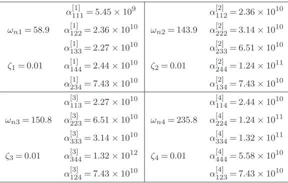
fori= 1,2, ..., N. The detailed model derivation process is given, for example, in [40]. Due to the geometry and boundary conditions of the plate, only cubic nonlinearity terms appear in Eq. (5.1). In this paper, we consider the same plate investigated in [45]. The geometrical and material properties of the plate and the values of the natural frequencies and nonlinear terms coefficients are given in AppendixA.

For this example plate, only its backbone curves are investigated, and also, it is assumed that the system is excited at a frequency in the vicinity of its second (and third) natural frequency. Considering just the first four eigenfrequencies (N= 4), there may exist a1 : 1resonant interaction between the second and third mode of the plate system becauseωn2≈ωn3. Therefore, it may not be possible to discern which of these two modes will be the dominant one, in order to construct the sparse vector of resonant states. Here, we may setu26= 0andu36= 0to represent the situation that an initial motion is initiated in either the second or third mode.

Following the approach in [45], and usinguˆ= [u2, u3]⊺, which reduces the system from a four-mode to a two-mode approximation, the vector of nonlinear terms is found to be

n(1)(ˆu)[2;3]=

α[2]₂₂₂(u3₂_p+u3₂_m+ 3u2₂_pu2m+ 3u2pu22m)

α[3]₃₃₃(u33p+u33m+ 3u23pu3m+ 3u3pu23m)

+α[2]₂₃₃(u2pu23p+u2mu23m+u2mu23p+u2pu23m+u2pu3pu3m+u2mu3pu3m)

+α[3]₂₂₃(u22pu3p+u22mu3m+u22pu3m+u22mu3m+u2pu2mu3p+u2pu2mu3m) !

,

(5.2)

where the subscript[2; 3]indicates the nonlinear terms inn₍₁₎associated with the second and third modes. Note that due to the specific value of the nonlinear coefficients, see Table2,n₍₁₎(ˆu)

[1]=n(1)(ˆu)[4]= 0 thus they are omitted. From Eq. (5.2), the vector of polynomials terms can be defined and its associatedβββ

matrix is computed as

u∗₍₁₎=                                       

u3₂_p u3₂_m u2₂_pu2m

u2pu22m

u2pu23p

u2mu23m

u2mu23p

u2pu23m

u2pu3pu3m

u2mu3pu3m

u22pu3p

u22mu3m

u2₂_pu3m

u22mu3m

u2pu2mu3p

u2pu2mu3m

u3₃_p u33m

3u2₃_pu3m

3u3pu23m                                       

, βββ⊺

(1)[2;3]=ω 2 r                                       8 8 8 8 0 0 0 0 8 8 8 8 0 0 0 0 0 0 0 0 8 8 8 8 0 0 0 0 0 0 0 0 8 8 8 8 0 0 0 0                                       , (5.3)

(18)

coefficients of non-resonant terms are computed, as

[n(1)]⊺[2;3]=                                                                    

α[2]₂₂₂ 0

3α[2]₂₂₂ 0

α[2]₂₃₃ 0

2α[2]₂₃₃ 0

2α[2]₂₃₃ 0 0 α[3]₂₂₃

0 α[3]₂₂₃

0 α[3₂₂₃

0 2α[3₂₂₃

0 2α[3]₂₂₃

0 α[3]₃₃₃

0 3α[3]₃₃₃

                                                                   

,[h(1)]⊺[2;3]= 1 8ωr2

                                                         

α[2]₂₂₂ 0

0 0

α[2]₂₃₃ 0

0 0

0 α[3]₂₂₃

0 0

0 α[3]₃₃₃

0 0 0 0                                                           . (5.4)

Using Eqs. (5.3) and (5.4), the vector of resonant and non-resonant nonlinear terms are determined as

n_u_(1)[2;3]= 3α [2]

222(u22pu2m+u2pu22m)

3α[3]₃₃₃(u23pu3m+u3pu23m)

+α[2]₂₃₃(u2mu32p+u2pu23m+ 2u2pu3pu3m+ 2u2mu3pu3m)

+α[3]₂₂₃(u2₂_pu3m+u22mu3p+ 2u2pu2mu3p+ 2u2pu2mu3m) !

,

(5.5)

h_(1)[2;3]= 1 8ω2

r

α[2]₂₂₂(u3₂_p+u3₂_m) +α[2]₂₃₃(u2pu23p+u2pu23p)

α[3]₃₃₃(u33p+u33m) +α [3]

223(u22pu3p+u22mu3m) !

. (5.6)

Finally, the time-invariant equations governing the response frequencies and amplitudes of the second and third modes are found to be,

"

ω2n2−ωr2+

3 4α [2] 222U 2 2+

2 + ei(φ3−φ2)

4 α [2] 233U 2 3 # U2

2 = 0, (5.7a) "

ω2n3−ωr2+3₄α[23333U 2 3+2 + e

i(φ2−φ3)

4 α [3] 223U 2 2 # U3

(19)

18

rs

p

a

.ro

ya

ls

o

c

ie

ty

p

u

b

lis

h

in

g

.o

rg

P

ro

c

R

S

o

c

A

0

..

Successively settingU3= 0andU2= 0results in the expressions of two single-mode (i.e. non-internally-resonant) backbone curves given by

S2 : ω_r2=ω_n2₂+ 3 4α

[2]

222U22, (5.8a)

S3 : ω_r2=ω_n2₃+ 3 4α

[3] 333U

2

3. (5.8b)

Combining the bracketed contents in Eqs. (5.7) and rearranging gives the expression of the double-mode (i.e. internally-resonant) backbone curves, written as

D₂₃± _:

      

     

U₃2=4 3

ω_n23−ω2n2

α[2]₂₃₃−α[3]₃₃₃

+α [3] 223−α

[2] 222

α[2]₂₃₃−α[3]₃₃₃ U₂2

ω2r=

α[2]₂₃₃ω2_n3−α[3]333ω 2 n2

α[2]₂₃₃−α[3]₃₃₃ +

3 4

α[2]₂₃₃α[3]₂₂₃−α[2]₂₂₂α[3]₃₃₃ α[2]₂₃₃−α[3]₃₃₃ U

2 2

, (5.9)

where, for balancing the complex terms,ei(|φ3−φ2)|_{= 1, the phase relationships}_φ

3−φ2= 0orπ, are assumed, which means there are two double-mode backbone curves with identical response frequencies and amplitudes but of different modal phase differences denoted by the superscript ofD₂₃±. See also [22] for a comparison of these results.

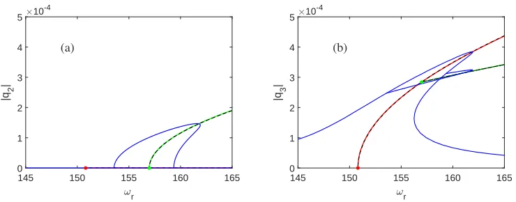
Fig. 4 shows the analytically approximated backbone curve results of the example plate using the coefficient values in Table 2. Again, the results from numerical continuation serve as the benchmark solution. The plate is assumed to be forced in the third (linear) mode-shape only. The frequency is set to be close to the second/third eigenfrequency, and the forcing amplitude is specifically chosen to make the resonant amplitude close to the thickness of the plate, i.e. f3= 0.02, which will ensure that the large-amplitude response assumption is satisfied.

Fig.4shows that the double-mode backbone curves,D23±, bifurcate from the single-mode backbone curve,S3. Note that as the results are projected in the modal coordinates, the two double-mode backbone curves overlap (as opposed to being in theu2,u3coordinate space). As we are forcing the system only in mode 3, theq3responses are driven by the external forcing, and has a hardening response curve (Fig.4(b)) as would be expected for a system with cubic nonlinearity. Theq2response (Fig.4(a)) is only triggered after theD₂₃± curves bifurcate from theS3 curve at an amplitude of approximatelyq3= 2.9×10−4. In contrast with the previous example, here the amplitudes are10−3smaller, and as a result the analytically computed backbone curve matches very accurately with the numerical solution, for both the single- and double-mode responses.

6. Conclusion

In this paper, we introduced a technique with the ability to perform a simultaneous direct normal form transform and model order reduction for nonlinear dynamic problems. This method is derived via its application to a general N-degree-of-freedom system of coupled oscillators with polynomial type nonlinearities. The main advantages of this new method are that (i) it is directly applicable to systems of second-order ordinary differential equations which are the natural description form of mechanical structures and (ii) it significantly simplifies the derivation process of the normal form transformation when applied to larger-scale systems. However, it should also be noted that model order reduction methods of this type will, by definition, neglect part of the system behaviour (often called the residual), and therefore care should be exercised to ensure that all the required dynamic behaviour is appropriately captured by the reduced order model. In our case, this was done by verifying the model using numerical continuation simulations of the forced damped system.

(20)

19

rs

p

a

.ro

ya

ls

o

c

ie

ty

p

u

b

lis

h

in

g

.o

rg

P

ro

c

R

S

o

c

A

0

..

145 150 155 160 165

r

0 1 2 3 4 5

|q2

|

10-4

(a)

145 150 155 160 165

r

0 1 2 3 4 5

|q3

|

10-4

[image:20.595.115.485.111.256.2]

(b)

Figure 4.The backbone curves and resonance curves of the example plate system. The solid-red and green lines

denote the analytically approximated backbone curvesS3 andD

±

23 respectively. The solid-black and blue lines are

the numerically computed backbone curves and forced responses (using COCO), respectively. The red and green dots

denote the branch points. Note that the information on the stability of the solution curves is not indicated on this figure.

Also note that the unit of the response amplitude,|qi|, is metres and the plate thickness is5×10−₄

m. The units ofωr

is radians/second.

dynamic behaviour. However, as we demonstrated, this can be done whilst simultaneously reducing the system from two- to one-degrees-of-freedom. As a result, all the intermediate matrices constructed during the nonlinear transform and the final resulting equation of motion were significantly simplified without sacrificing the accuracy of the solution. The approximated backbone curves results were then shown to be able to accurately predict the softening behaviour and the resonant response of the example system when harmonically forced, by comparison with numerical continuation simulations of the forced damped system. Finally, the application of the new method to the example of a thin, rectangular, simply-supported plate was investigated. Due to the specific geometry and boundary conditions of the plate, there exists a 1:1 internal resonance between the second and third modes of the system. In previous work, a four-mode reduced order model was used to explain this behaviour. However, by using the reduced-order-direct normal form, only the two interacting modes were required to capture the key dynamic behaviour. Accordingly, the dynamics of the plate system were reduced to a system of two resonantly interacting oscillators. The associated numerical continuation results show a high degree of consistency with the analytically obtained backbone curve solutions for both single-mode and resonant double-mode responses.

Data Accessibility. The datasets supporting this article have been uploaded as part of the supplementary material.

Authors’ Contributions. Both authors contributed equally to this work.

Funding. The authors would like to acknowledge the support of the Engineering and Physical Science Research Council. This work was started while D.J.W was supported by EPSRC grant EP/K003836/2, and finished under the grant EP/R006768/1. X. L. was supported by a Department of Mechanical Engineering studentship and also EPSRC grant EP/J016942/1.

Acknowledgements. The authors would also like to thank Ayman Nasir for assistance in proof reading the manuscript.

Simultaneous normal form transformation and model-order reduction for systems of coupled nonlinear oscillators

This is a repository copy of

Simultaneous normal form transformation and model-order

reduction for systems of coupled nonlinear oscillators

.

White Rose Research Online URL for this paper:

http://eprints.whiterose.ac.uk/148394/

Version: Accepted Version

Article:

Liu, X. and Wagg, D. orcid.org/0000-0002-7266-2105 (2019) Simultaneous normal form

transformation and model-order reduction for systems of coupled nonlinear oscillators.

Proceedings of the Royal Society A: Mathematical, Physical and Engineering Sciences,

475 (2228). ISSN 1364-5021

https://doi.org/10.1098/rspa.2019.0042

© 2019 The Authors. This is an author-produced version of a paper accepted for

publication in Proceedings of the Royal Society A: Mathematical, Physical and Engineering

Sciences. Uploaded in accordance with the publisher's self-archiving policy.

[email protected]

https://eprints.whiterose.ac.uk/

Reuse

Items deposited in White Rose Research Online are protected by copyright, with all rights reserved unless

indicated otherwise. They may be downloaded and/or printed for private study, or other acts as permitted by

national copyright laws. The publisher or other rights holders may allow further reproduction and re-use of

the full text version. This is indicated by the licence information on the White Rose Research Online record

for the item.

Takedown

If you consider content in White Rose Research Online to be in breach of UK law, please notify us by

rspa.royalsocietypublishing.org

Research

Simultaneous normal form

transformation and

model-order reduction for

systems of coupled nonlinear

oscillators

X. Liu

, and D. J. Wagg

1. Introduction

2. Direct normal form method

3. An order-reduced variant of the nonlinear transform

4. Example 1: a two-degree-of-freedom discrete mass-spring

system

5. Example 2: a continuous plate system

6. Conclusion

A. The parameters of the example plate