Generating maximal entanglement between spectrally distinct solid-state emitters

solid-state emitters

.

White Rose Research Online URL for this paper:

http://eprints.whiterose.ac.uk/141185/

Version: Submitted Version

Article:

Hurst, D.L., Joanesarson, K.B., Iles-Smith, J. et al. (2 more authors) (Submitted: 2019)

Generating maximal entanglement between spectrally distinct solid-state emitters. arXiv.

(Submitted)

© 2019 The Author(s). For reuse permissions, please contact the Author(s).

[email protected] https://eprints.whiterose.ac.uk/ Reuse

Items deposited in White Rose Research Online are protected by copyright, with all rights reserved unless indicated otherwise. They may be downloaded and/or printed for private study, or other acts as permitted by national copyright laws. The publisher or other rights holders may allow further reproduction and re-use of the full text version. This is indicated by the licence information on the White Rose Research Online record for the item.

Takedown

If you consider content in White Rose Research Online to be in breach of UK law, please notify us by

Generating maximal entanglement between spectrally distinct solid-state emitters

David L. Hurst†_,1 _{Kristoffer B. Joanesarson}†_,1, 2 _{Jake Iles-Smith,}1 _{Jesper Mørk,}2 _{and Pieter Kok}1,∗

1_{Physics & Astronomy, University of Sheffield, Hounsfield Road, Sheffield, S3 7RH, United Kingdom} 2_{Department of Photonics Engineering, Technical University of Denmark, Ørsteds Plads, Lyngby, Denmark}

(Dated: January 14, 2019)

We show how to create maximal entanglement between spectrally distinct solid-state emitters em-bedded in a waveguide interferometer. By revealing the rich underlying structure of multi-photon scattering in emitters, we show that a two-photon input state can generate deterministic maximal entanglement even for emitters with significantly different transition energies and line-widths. The optimal frequency of the input is determined by two competing processes: which-path erasure and interaction strength. We find that smaller spectral overlap can be overcome with higher photon numbers, and quasi-monochromatic photons are optimal for entanglement generation. Our work provides a new methodology for solid-state entanglement generation, where the requirement for perfectly matched emitters can be relaxed in favour of optical state optimisation.

Quantum technologies promise dramatic improvements in computing and communication by utilizing quantum entanglement between qubits. Although many promising quantum technology architectures have emerged over the last two decades, none are free from the practical chal-lenges presented by high-fidelity quantum control and scalability. For example, superconducting circuit imple-mentations enjoy excellent coherence properties but op-erate slowly [1], while trapped ion qubits can be prepared with almost unit fidelity but are difficult to scale [2]. Solid state architectures, such as optically coupled spin systems, compete on speed and scalability. They include semiconductor quantum dots and nitrogen-vacancy cen-tres. Large optical non-linearities in solid-state systems are now very common [3–5], and solid-state emitters are readily integrated into complex photonic structures, fur-ther enhancing the light-matter interaction [6]. However, there are many challenges still to overcome. For exam-ple, charge noise and phonon scattering have limited the size of the optical non-linearities observed thus far [3].

Another major drawback to solid-state emitters is that the central energies and lifetimes of their transitions are highly dependent on the fabrication process, and vary significantly both across and within samples [7]. Known methods for entangling solid-state qubits require emit-ters with identical energies to facilitate path-erasure tech-niques [8, 9]. This adds a practically insurmountable overhead to the process of matching multiple solid-state qubits for creating large entangled states [10]. Stark shifting and strain tuning the emitter transitions has been employed to tune solid-state emitters onto reso-nance [11–13], but this requires a substantial technical overhead and arbitrary emitters in a sample cannot in general be tuned onto resonance. Here, we propose a pro-cess for generating entanglement that is robust against spectral variations in the emitters’ transition energies and line-widths. We show that photons, linear optics, and photon counting suffice to create deterministic entangle-ment between imperfectly matched emitters, revealing a rich underlying structure of multi-photon scattering off

p

[image:2.612.321.558.250.380.2]

q

|

e

_⟩

|↑⟩ |↓⟩

E

1

|

n

_⟩

|

m

_⟩

D

1

D

2

1

2

BS

1

BS

2

γ

1

Γ

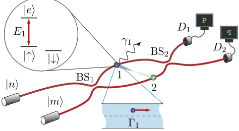
1

FIG. 1. Waveguide Mach-Zehnder interferometer with emit-ters embedded at positions 1 and 2, and with L-type level structures shown in the inset. The excited state |ei is cou-pled to a spin qubit state (e.g., |↑i) with transition energy

Eα (α= 1,2), circular polarisation, and line-width Γα. The

emitters are placed off-axis in the waveguide at c-points, such that circularly polarised light scatters only in the forward di-rection. The loss rate from the guided mode isγα. Fock states

|n, miare injected into the interferometer, and detectors D1

andD2 record a photon number detector signature (p, q).

two non-identical emitters. While many challenges re-main, this work removes a major obstacle to a scalable solid state quantum technology architecture.

Our setup is shown in Fig.1. Two solid-state emitters each have anL-type level structure, with two stable low-lying spin states (|↑⟩, |↓⟩), and a dipole transition that couples a spin state to an excited state|e⟩. The transition energy for emitterα= 1,2 isEα, and the polarisation is circular due to selection rules. The emitters are initially prepared in the product state (|↑⟩+|↓⟩)(|↑⟩+|↓⟩)/2, and embedded in a waveguide Mach-Zehnder interferometer at c-points, where perfect correlation between propaga-tion direcpropaga-tion and circular polarisapropaga-tion occurs [14]. Con-sequently, the emitters scatter circularly polarised light only in the forward direction, as was demonstrated re-cently using semiconductor quantum dots under an

plied magnetic field [15–18]. For a lossless waveguide, the emitter will impart a π-phase shift to each photon that is on resonance with the transition [19–22]. The input to the interferometer is a two-mode Fock state |n, m⟩, and the detectors D1 and D2 produce classical

signa-tures (p, q) indicating the presence of pand q photons, respectively.

Assuming the emitters are identical, a single monochromatic resonant photon injected into ei-ther one of the input arms of the interferome-ter will scatinterferome-ter from one of the emitinterferome-ters, and af-ter the final beam splitaf-ter the light-mataf-ter degrees of freedom are in the multi-partite entangled state (|Φ−_{⟩ ⊗ |1,0⟩ − |Ψ}−_{⟩ ⊗ |0,1⟩)/}√_{2, where|0,1⟩and|1,0⟩}

is the two-mode single photon state at the interfer-ometer output. A photon detector signature (1,0) or (0,1) heralds the maximally entangled spin state|Φ−_⟩=

(|↑,↑⟩ − |↓,↓⟩)/√2 or |Ψ−_{⟩= (|↑,↓⟩ − |↓,↑⟩)/}√_{2. This}

method can be made robust to photon loss provided that the emitter detuning is only a fraction of the emitter line-width. Mahmoodianet al. showed how this can form a building block for distributed quantum computing [23].

In practice, both the line-widths and transition ener-gies vary significantly between solid-state emitters, and it was generally assumed that this prohibits the creation of perfect entanglement using linear optics and photode-tection. In this case, the input photon can no longer be resonant with both emitters simultaneously. With ¯hωthe single-photon energy, Γαthe unidirectional emission rate of emitter α= 1,2 into the waveguide, and γα the cor-responding coupling to non-guided modes, the scattering process is described by the transmission coefficient [24]

tα(ω) =¯hω−Eα−i¯h(Γα−γα)/2 ¯

hω−Eα+i¯h(Γα+γα)/2

. (1)

We characterise the emitter loss byβα≡Γα/(Γα+γα). For non-zero emitter detuningδ≡E2−E1,tα(ω) ceases to be aπphase shift, and forβα<1,tα(ω) is no longer a pure phase shift. The setup then does not create maxi-mally entangled states deterministically anymore. Never-theless, we will now demonstrate how tailoring the opti-cal input state|n, m⟩into the Mach-Zehnder interferome-ter leads to deinterferome-terministic maximal entanglement between two spectrally distinct emitters.

In general, a detector signature (p, q) indicates that the two emitters are in a mixed entangled state. We use the concurrenceC(ρ) for a two-qubit stateρto quantify this entanglement [25]. Each signature (p, q) occurs with probability Pr(p, q) and results in an emitter stateρ(p,q),

leading to a concurrenceC(ρ(p,q)). We define theaverage

concurrence as

Cavg≡

X

(p,q)

Pr(p, q)C ρ(p,q)

. (2)

This is an appropriate figure of merit, since it provides a lower bound for the amount of entanglement expected

from a given experiment without post-selection. The en-tanglement in the two-qubit state can be increased by dis-carding measurement outcomes corresponding to below-average concurrences. This comes at the expense of the rate of entanglement generation.

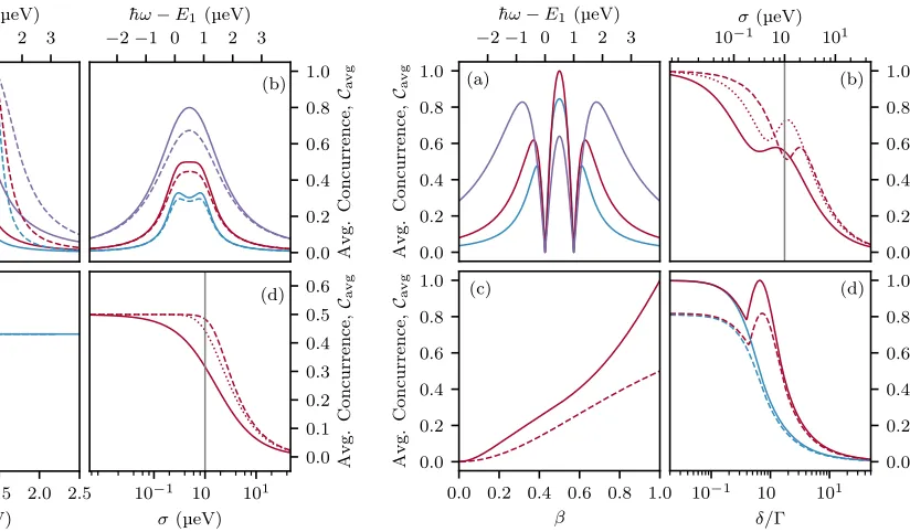
The amount of entanglement that can be generated between the two spectrally distinct emitters with a sin-gle probe photon is shown in Fig. 2. The single pho-ton protocol is analysed using linear optics transforma-tions [23], while a multiphoton input requires taking into account the non-linear nature of the interaction [21] (see SI for details). As expected, for spectrally distinct emit-ters the average concurrence does not reach its maximal value [Fig.2(b)]. The amount of entanglement is deter-mined by two competing processes. On the one hand, which-path information for the probe photon must be erased, while at the same time the phase shift induced by the photon scattering event must be maximised. Tun-ing closer to either emitter increases the relative phase shift but also imparts a degree of path information onto the probe, as the light-matter interaction is now stronger for one of the emitters. For emitters with finite detun-ing and line-width it is not obvious which photon energy maximises the average concurrence. Three emitter line-widths are shown in Fig. 2(a), and Fig. 2(b) shows the corresponding Cavg. The linewidths shown correspond

to emitters with 1, 0.66 and 0.33 ns lifetimes, typical of semiconductor QDs benefiting from modest Purcell en-hancements [26]. Increasing the line-width of the emit-ters leads to a larger spectral overlap, thereby erasing some of the which-path information and increasingCavg.

Fig.2(c) shows the optimal frequency of the input pho-ton that maximises Cavg. For narrow line-widths it is

preferable to tune the photon energy away from the mean emitter energy (¯hω−E1= 0.5µeV forδ= 1.0µeV), and towards resonance with one of the emitters. Though this reduces the concurrence in the state heralded by a click at detectorD2, it does increase the probability of a

suc-cessful scattering event.

One may expect that a photon with a wide frequency bandwidth that overlaps with both emitters will im-prove the entanglement generation. Fig. 2(d) shows the average concurrence for a single probe photon with Lorentzian, Gaussian and square spectral profiles, cen-tred at ¯hω = E1 +δ/2, as a function of the photon

3

−2−1 0 1 2 3 ¯

h!−E1(µeV)

0.0

0.2

0.4

0.6

0.8

1.0

In

tensit

y

(a.u.)

(a)

−2−1 0 1 2 3 ¯

h!−E1 (µeV)

0.0

0.2

0.4

0.6

0.8

1.0

Avg.

Concurrence,

Ca

vg

(b)

0.0 0.5 1.0 1.5 2.0 2.5

Γ (µeV)

0.0

0.1

0.2

0.3

0.4

0.5

0.6

0.7

¯ h! opt − E1 ( µ eV) (c)

10−1 ₁₀0 ₁₀1

σ(µeV)

0.0

0.1

0.2

0.3

0.4

0.5

0.6

Avg.

Concurrence,

Ca

vg

[image:4.612.64.361.49.289.2]

(d)

FIG. 2. Single-photon (e.g.,|1,0i) entanglement generation for a pair of detuned L-type emitters with equal line-width Γ and energiesE1 and E2=E1+δ, whereδ = 1.0µeV. (a)

Lorentzian spectra for emitters with energiesE1 (solid), E2

(dashed), and emitter line-widths 0.66 µeV (blue), 1.0 µeV

(red), and 2.0 µeV (purple). (b) Average concurrence

ver-sus monochromatic single-photon energy without loss (β =

β1 =β2 = 1, solid) and with loss (β = 0.9, dashed). Line

colours as in (a). (c) Location of optimum single-photon en-ergy ¯hωopt for maximum Cavg as a function of emitter

line-width Γ for a monochromatic input without loss (solid) and withβ= 0.9 (dashed). (d)Cavg for Lorentzian (solid),

Gaus-sian (dotted), and square (dashed) single-photon envelopes as a function of FWHM pulse-widthσ. Here, ¯hω= (E1+E2)/2

and Γ = 1.0µeV. The vertical line indicates the line-width of

the emitters.

Cavgof the single-photon case is limited by the competing

requirements of maximising the induced phase shift and path erasure.

Next, we consider whether two photons can increase the average concurrence. Consider an input state of two identical monochromatic photons|n, m⟩=|1,1⟩entering the interferometer. They will evolve into a two-photon noon state (|2,0⟩ − |0,2⟩)/√2 via Hong-Ou-Mandel in-terference on the first beam splitter [27] and interact with the emitters. Entanglement is then heralded by three detector signatures: two photons inD1, two

pho-tons in D2, or a coincidence count. Using two probe

photons leads to a rich structure in the average concur-rence, and it is now possible to reach deterministic max-imal entanglement for spectrally distinct emitters with finite line-width. The reason for the two-photon ad-vantage can be determined via inspection of Fig. 3(a), where Cavg is shown as a function of the detuning

be-−2−1 0 1 2 3 ¯

h!−E1(µeV)

0.0

0.2

0.4

0.6

0.8

1.0

Avg.

Concurrence,

Ca

vg _(a)

10−1 ₁₀0 ₁₀1

σ(µeV)

0.0

0.2

0.4

0.6

0.8

1.0

Avg.

Concurrence,

Ca

vg

(b)

0.0 0.2 0.4 0.6 0.8 1.0

β

0.0

0.2

0.4

0.6

0.8

1.0

Avg.

Concurrence,

Ca

vg _(c)

10−1 ₁₀0 ₁₀1

δ/Γ

0.0

0.2

0.4

0.6

0.8

1.0

Avg.

Concurrence,

Ca

vg

(d)

FIG. 3. Two-photon (i.e.,|1,1i) entanglement generation for a pair of detuned L-type emitters with equal line-width Γ and energies E1 and E2=E1+δ, where δ = 1.0 µeV. (a)

Average concurrence versus monochromatic two-photon en-ergy. The emitters have equal line-width of 0.66µeV (blue),

1.0µeV (red), and 2.0µeV (purple). (b)Cavg for Lorentzian

(solid), Gaussian (dotted), and square (dashed) single-photon envelopes as a function of FWHM pulse-width σ. Here, ¯

hω = (E1+E2)/2 and Γ = 1.0 µeV. The vertical line

in-dicates the line-width of the emitters. (c) Average concur-rence as a function of β = β1 = β2 for a monochromatic

two-photon pulse (solid) and monochromatic single-photon pulse (dashed); both emitters have line-widths of 1.0 µeV.

(d) Average concurrence as a function of normalised emitter detuningδ/Γ for two monochromatic photons (red) and a sin-gle monochromatic photon (blue). Solid lines representβ= 1 and dashed lines representβ= 0.9.

tween the photon energy and the transition energy of the first emitter. In the current example whereδ= 1.0µeV, maximum entanglement fidelity occurs for emitters with line-widths of 1.0 µeV and input photons with energy ¯

hω=E1+δ/2. Comparing this value to Fig.2(a), this

input energy corresponds to the point where the emitter spectra are at half of their maximum intensity. For quasi-monchromatic input states, the imparted phase shift is additive in photon number, i.e., for the two-photon case, each photon imparts aπ/2 phase shift to the emitter and therefore achieves the requiredπphase shift. We consider more general emitter detuning and line-width examples in Fig.4and in the Supplementary Information.

[image:4.612.140.552.50.291.2]

photons are present, the emitter may be excited, which opens a pathway for stimulated emission, such that the coherence of the wave-packet is maintained. Competi-tion between spontaneous and stimulated emission pro-cesses leads to the non-monotonic behaviour inCavg

pre-sented in Fig.3(b). The two-photon interaction strength increases when the optical pulse width is broadened to the scale of the emitter line-width [21]. Although an increased bandwidth generally reducesCavg, a local

max-imum appears close to the emitter line-width. We at-tribute this to the stimulated emission process, which is maximised for photons that are closely matched to the emitters’ spectral profile. Fig.3(c) shows the dependence ofCavg on the loss rateβ. The two-photon entanglement

generation process outperforms the single-photon process for all values ofβ. In Fig.3(d) we show howCavgdepends

on different two-photon pulse shapes.

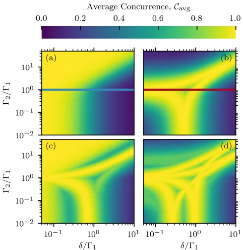
In certain regimes the two-photon process is capable of generating maximal entanglement between spectrally dis-tinct emitters where the single-photon process fails. We studied the robustness of this effect with respect to the system parameters. In Figs. 4(a) and4(b) we show the maximum Cavg (optimised over photon frequency ωopt)

for the one- and two-photon input states as a function of the emitter detuning and the emitter line-width ra-tio. The single-photon case outperforms the two-photon case if the emitters are spectrally collocated, or if one of the emitters significant overlaps the other, however nar-row the line-width. Crucially, however, by exploiting the multi-photon additivity of the phase shift, a two-photon process can efficiently generate entanglement forany fi-nite detuning without requiring arbitrarily small emit-ter lifetimes. The converse of this is also true: for any combination of line-widths Γ1and Γ2 there exists a

non-zero emitter detuning which creates deterministic max-imal entanglement given the optmax-imal two-photon input state. In practice, this means a much greater freedom in matching solid-state emitters for entanglement gener-ation in a Mach-Zehnder interferometer than previously thought.

We extended the entanglement generation process to monochromatic|n, m⟩ Fock states into the interferome-ter. In Figs.4(c) and4(d) we show the maximumCavgas

a function of the emitter detuning and the emitter line-width ratio for input states|2,1⟩and|2,2⟩, respectively (for more examples, see the Supplementary Information). There is a marked improvement in the entanglement gen-eration over the single- and two-photon processes, with larger areas of parameter space achieving a near-unity

Cavg. Remarkably, this indicates that a wide range of

im-perfections in the fabrication of two identical emitters can be overcome by optical state optimisation. Note that the

|2,1⟩case inherits features from both the|1,1⟩and|1,0⟩

[image:5.612.317.562.49.302.2]

processes. It therefore performs well for both spectrally collocated emitters and those with finite detuning. A similar compound structure is visible in Fig.4(d), where

FIG. 4. Maximum average concurrence for different photon number input states injected into the interferometer. The emitter detuningδand the line-width Γ2 are both normalised

to Γ1, and we consider lossless waveguides (β = 1). The

input photons are identical and monochromatic in the con-figurations (a)|1,0i; (b)|1,1i; (c) |2,1i; and (d)|2,2i. The characteristic shapes in (a) and (b) recur in (c) and (d), and are also found in higher photon number input states|n, mi. The blue and red lines in (a) and (b) correspond respectively to the solid blue and red lines in Fig.3(d).

an input state|2,2⟩shows a double two-photon structure compared to the|1,1⟩input in Fig. 4(b). A clear trend emerges, where larger spectral emitter detuning can be overcome by higher number input states|n, m⟩(see Sup-plementary Information).

5

spin-doped solid-state emitters is nuclear spin interac-tions [31]. While this naturally leads to a random pre-cession of the spin ground-state, there are a number of strategies based on dynamical decoupling that may be used to suppress its impact [32–34]. In addition, solid-state emitters are subject to charge fluctuations and phonon interactions. The former leads to spectral wandering occurring on a microsecond timescale, which may be overcome by operating the process on shorter timescales [35]. Phonon scattering leads to sidebands [36] that can be removed through frequency filtering or by placing the emitter in an optical cavity [37,38].

In conclusion, we presented a robust entanglement gen-eration mechanism between two solid-state qubits em-bedded in a Mach-Zehnder interferometer. Entangling techniques that use solid-state emitters are well-known to place very stringent requirements on the spectral iden-tity of the emitters [8]. Our approach overcomes these restrictions by showing how to tailor multi-photon input states, mitigating a long considered weakness of solid-state emitters. We found that maximal deterministic entanglement between increasingly distinct emitters is possible using higher photon number input states, re-vealing a rich structure in multi-photon scattering from two emitters with different energies and line-widths. Our work provides a new methodology for solid-state entan-glement generation, where the requirement for perfectly matched emitters can be relaxed in favour of optical state optimisation.

Acknowledgements.— the authors thank A.P. Foster, D. Hallett, and M.S. Skolnick for useful suggestions, and EPSRC for financial support. K.B.J and J.M. acknowl-edge funding from the Danish Council for Independent Research (DFF-4181-00416). J.I.S. is supported by the Royal Commission for the Exhibition of 1851.

†_{DLH and KBJ contributed equally to this project.}

∗ _{[email protected]}

[1] G. Wendin,Rep. Prog. Phys.80, 106001 (2017). [2] D. Kielpinski, C. Monroe, and D. J. Wineland,Nature

417, 709 (2002).

[3] D. Hallett, A. P. Foster, D. L. Hurst, B. Royall, P. Kok, E. Clarke, I. E. Itskevich, A. M. Fox, M. S. Skolnick, and L. R. Wilson,Optica5, 644 (2018).

[4] A. Javadi, I. S¨ollner, M. Arcari, S. L. Hansen, L. Midolo, S. Mahmoodian, G. Kirˇsansk˙e, T. Pregnolato, E. H. Lee, J. D. Song, S. Stobbe, and P. Lodahl,Nature Comms.

6, 8655 EP (2015).

[5] A. Sipahigil, R. E. Evans, D. D. Sukachev, M. J. Bu-rek, J. Borregaard, M. K. Bhaskar, C. T. Nguyen, J. L. Pacheco, H. A. Atikian, C. Meuwly, R. M. Camacho, F. Jelezko, E. Bielejec, H. Park, M. Lonˇcar, and M. D. Lukin,Science354, 847 (2016).

[6] P. Lodahl, S. Mahmoodian, and S. Stobbe,Rev. Mod.

Phys.87, 347 (2015).

[7] P. Michler, Single Semiconductor Quantum Dots, NanoScience and Technology (Springer Berlin Heidel-berg, 2009).

[8] S. D. Barrett and P. Kok, Phys. Rev. A 71, 060310

(2005).

[9] J. Metz and S. D. Barrett, Phys. Rev. A 77, 042323

(2008).

[10] R. Raussendorf and H. J. Briegel,Phys. Rev. Lett. 86,

5188 (2001).

[11] R. Stockill, M. J. Stanley, L. Huthmacher, E. Clarke, M. Hugues, A. J. Miller, C. Matthiesen, C. Le Gall, and M. Atat¨ure,Phys. Rev. Lett.119, 010503 (2017). [12] H. Bernien, B. Hensen, W. Pfaff, G. Koolstra, M. S.

Blok, L. Robledo, T. H. Taminiau, M. Markham, D. J. Twitchen, L. Childress, and R. Hanson,Nature497, 86

(2013).

[13] B. Hensen, H. Bernien, A. E. Dr´eau, A. Reiserer, N. Kalb, M. S. Blok, J. Ruitenberg, R. F. L. Vermeulen, R. N. Schouten, C. Abell´an, W. Amaya, V. Pruneri, M. W. Mitchell, M. Markham, D. J. Twitchen, D. Elkouss, S. Wehner, T. H. Taminiau, and R. Hanson, Nature

526, 682 (2015).

[14] P. Lodahl, S. Mahmoodian, S. Stobbe, A. Rauschenbeu-tel, P. Schneeweiss, J. Volz, H. Pichler, and P. Zoller,

Nature541, 473 (2017).

[15] I. S¨ollner, S. Mahmoodian, S. L. Hansen, L. Midolo, A. Javadi, G. Kirˇsansk˙e, T. Pregnolato, H. El-Ella, E. H. Lee, J. D. Song, S. Stobbe, and P. Lodahl,Nature

Nan-otech.10, 775 (2015).

[16] R. J. Coles, D. M. Price, J. E. Dixon, B. Royall, E. Clarke, P. Kok, M. S. Skolnick, A. M. Fox, and M. N. Makhonin,Nature Comms.7, 1 (2016).

[17] B. Lang, R. Oulton, and D. M. Beggs,J. Opt.19, 045001

(2017).

[18] D. L. Hurst, D. M. Price, C. Bentham, M. N. Makhonin, B. Royall, E. Clarke, P. Kok, L. R. Wilson, M. S. Skol-nick, and A. M. Fox,Nano Lett.18, 5475 (2018). [19] S. Fan, S. E. Kocabas, and J.-T. Shen,Phys. Rev. A82,

063821 (2010).

[20] A. Roulet and V. Scarani, New J. Phys. 18, 093035

(2016).

[21] A. Nysteen, D. P. S. McCutcheon, M. Heuck, J. Mørk, and D. R. Englund,Phys. Rev. A95, 062304 (2017). [22] D. L. Hurst and P. Kok,Phys. Rev. A97, 043850 (2018). [23] S. Mahmoodian, P. Lodahl, and A. S. Sørensen,Phys.

Rev. Lett.117, 240501 (2016).

[24] E. Rephaeli and S. Fan,Photon. Res.1, 110 (2013). [25] W. K. Wootters,Phys. Rev. Lett.80, 2245 (1998). [26] S. Hughes,Opt. Lett.29, 2659 (2004).

[27] C. K. Hong, Z. Y. Ou, and L. Mandel,Phys. Rev. Lett.

59, 2044 (1987).

[28] A. Divochiy, F. Marsili, D. Bitauld, A. Gaggero, R. Leoni, F. Mattioli, A. Korneev, V. Seleznev, N. Kaurova, O. Mi-naeva, G. Gol’tsman, K. Lagoudakis, M. Benkhaoul, F. L´evy, and A. Fiore,Nature Phot.2, 302 (2008). [29] R. M. Heath, M. G. Tanner, T. D. Drysdale, S. Miki,

V. Giannini, S. A. Maier, and R. H. Hadfield, Nano

Lett.15, 819 (2015).

[30] D. N. Klyshko, A. N. Penin, and B. F. Polkovnikov, JETP Lett.11, 5 (1970).

[31] I. A. Merkulov, A. L. Efros, and M. Rosen,Phys. Rev.

B65, 205309 (2002).

[32] L. Viola, E. Knill, and S. Lloyd,Phys. Rev. Lett. 82,

[33] D. Press, K. De Greve, P. L. McMahon, T. D. Ladd, B. Friess, C. Schneider, M. Kamp, S. H¨ofling, A. Forchel, and Y. Yamamoto,Nature Phot.4, 367 EP (2010). [34] A. V. Kuhlmann, J. Houel, A. Ludwig, L. Greuter,

D. Reuter, A. D. Wieck, M. Poggio, and R. J. War-burton,Nature Phys.9, 570 EP (2013).

[35] A. Berthelot, I. Favero, G. Cassabois, C. Voisin, C. De-lalande, P. Roussignol, R. Ferreira, and J. M. G´erard,

Nature Phys.2, 759 EP (2006).

[36] J. Iles-Smith, D. P. S. McCutcheon, J. Mørk, and A. Nazir,Phys. Rev. B95, 201305 (2017).

[37] T. Grange, N. Somaschi, C. Ant´on, L. De Santis, G. Cop-pola, V. Giesz, A. Lemaˆıtre, I. Sagnes, A. Auff`eves, and P. Senellart,Phys. Rev. Lett.118, 253602 (2017). [38] J. Iles-Smith, D. P. S. McCutcheon, A. Nazir, and

Supplemental Information: Generating maximal entanglement between spectrally

distinct emitters

David L. Hurst,1 _{Kristoffer B. Joanesarson,}1, 2 _{Jake Iles-Smith,}1 _{Jesper Mørk,}2 _{and Pieter Kok}1

1_{Department of Physics and Astronomy, University of Sheffield,} Hounsfield Road, Sheffield, S3 7RH, United Kingdom

2_{Department of Photonics Engineering, Technical University of Denmark, Ørsteds Plads, Lyngby, Denmark}

(Dated: January 14, 2019)

FIGURE OF MERIT

Concurrence is the entanglement measure we choose, as it permits a natural extension to states that can only be described in terms of a density matrix [1]. For the two-qubit mixed state ρ, the concurrence is found via

C(ρ) = max(0, λ1−λ2−λ3−λ4), (1)

whereλi is theith _{eigenvalue of}

R(ρ) =

q_√

ρσ(1)y ⊗σ(2)y ρ∗σ(1)y ⊗σy(2)√ρ, (2) arranged in decreasing order. For a pure two-qubit state |φ⟩the expression for the concurrence can be written as

C(|φ⟩) =| hφ|σy(1)⊗σ(2)y |φ∗⟩ |. In the projection-by-measurement type protocol, the probability that detector 1 (D1)

and 2 (D2) gives pand q clicks, respectively, is Pr(p, q). The detection outcome heralds the qubit state ρ(p,q), and

C ρ(p,q)

is the associated concurrence. The single set (p, q) corresponds to one of the possible detection outcomes where the number of possible outcomes depends on the number of incident photons, whether the detectors are number resolving or not, and whether photon-loss is present. We define the average concurrence as the figure of merit and this is given by

Cavg≡

X

(p,q)

Pr(p, q)C ρ(p,q)

. (3)

SINGLE-PHOTON PROTOCOL

Single-photon transport in the MZI

The initial two-qubit state is taken to be the separable pure state

|φin⟩=

1

2(|↑⟩+|↓⟩)⊗(|↑⟩+|↓⟩). (4)

We choose a single-photon input state with the photon injected into the upper arm of the Mach-Zehnder Interferometer (MZI). The optical state is

|ψin⟩=

Z

dω ξ(ω)u†(ω)|∅_{⟩, (5)}

whereu(ω) is the annihilation operator for a photon of frequencyωin the upper interferometer arm andξ(ω) describes the optical wavepacket, such thatR

dω|ξ(ω)|2= 1. The photon state after scattering off the first beam-splitter (BS) is

|ψ2⟩=

Z

dω ξ(ω)√1

2

u†_{(ω) +d}†_(ω)

|∅_{⟩, (6)}

whered(ω) is the annihilation operator for the lower interferometer arm. The combined photon-emitter state is

|Ψ2⟩=|φin⟩ ⊗ |ψ2⟩=

1

2(|↑⟩+|↓⟩)⊗(|↑⟩+|↓⟩)⊗

Z

dω ξ(ω)√1

2

u†_{(ω) +d}†_(ω)

|∅_{⟩. (7)}

After scattering off the emitters we find that the state evolves to

|Ψ3⟩=

1 2√2

Z

dω ξ(ω)(t1(ω)|↑⟩+|↓⟩)⊗(|↑⟩+|↓⟩)⊗u†(ω)|∅⟩

+ 1

2√2

Z

dω ξ(ω)(|↑⟩+|↓⟩)⊗(t2(ω)|↑⟩+|↓⟩)⊗d†(ω)|∅⟩,

(8)

where t1(ω) and t2(ω) are the transmission coefficients for a photon of frequency ω scattering from the emitter at

position 1 and 2, respectively (defined in the main text). The photon state after the second BS and before measurement is

|Ψ4⟩=

1 4

Z

dω ξ(ω)

[t1(ω) +t2(ω)]|↑,↑⟩+ [t1(ω) + 1]|↑,↓⟩+ [1 +t2(ω)]|↓,↑⟩+ 2|↓,↓⟩

⊗u†_(ω)|∅⟩

+1 4

Z

dω ξ(ω)

[−t1(ω) +t2(ω)]|↑,↑⟩+ [−t1(ω) + 1]|↑,↓⟩+ [−1 +t2(ω)]|↓,↑⟩

⊗d†_(ω)|∅⟩

(9)

Single-photon measurement

We define our positive operator-valued measures (POVMs) used to determine the detection probabilities and post measurement states. The single-photon POVMs are

Π(u) =

Z

dω u†_{(ω)|∅⟩h∅|u(ω), (10a)}

Π(d) =

Z

dω d†_{(ω)|∅⟩h∅|d(ω). (10b)}

The detection probabilities associated with the POVMs and the corresponding post-measurement states are given by [2]

Pr(p, q) = hΨ4|Π(updq)|Ψ4⟩, and

Ψ

′

(p,q)

E

= p 1

Pr(p, q)Π(u p_dq_)|Ψ

4⟩, (11)

respectively. Using the state in Eq. (9), the probability of detecting one photon atD1is

Pr(1,0) = 1 16

Z

dω |ξ(ω)|2 _|t

1(ω) +t2(ω)|2+|t1(ω) + 1|2+|1 +t2(ω)|2+ 4, (12)

and atD2is

Pr(0,1) = 1 16

Z

dω|ξ(ω)|2 _{| −t}

1(ω) +t2(ω)|2+| −t1(ω) + 1|2+| −1 +t2(ω)|2. (13)

We find the two-qubit state by tracing out the waveguide modes. This gives us the density matrices

ρ(1,0)=

Z

dω |ξ(ω)|2

φ(1,0)(ω)φ(1,0)(ω)

, (14)

and

ρ(0,1)=

Z

dω |ξ(ω)|2

φ(0,1)(ω)

φ(0,1)(ω)

, (15)

where

φ(1,0)(ω)=

1 4p

Pr(1,0)

[t1(ω) +t2(ω)]|↑,↑⟩+ [t1(ω) + 1]|↑,↓⟩+ [1 +t2(ω)]|↓,↑⟩+ 2|↓,↓⟩

, (16)

and

φ(0,1)(ω)=

1 4p

Pr(0,1)

[−t1(ω) +t2(ω)]|↑,↑⟩+ [−t1(ω) + 1]|↑,↓⟩+ [−1 +t2(ω)]|↓,↑⟩

. (17)

3

Monochromatic single-photon input

For a monochromatic input-photon with frequency ω, the two density operators describing the heralded two-qubit states can be reduced to pure states. For the probabilities and corresponding two-qubit states we find the following simplified results. With a probability of

Pr(1,0) = 1

16 |t1(ω) +t2(ω)|

2₊

|t1(ω) + 1|2+|1 +t2(ω)|2+ 4

, (18)

we detect a photon atD1 and thus herald the two-qubit state

φ_(1,0)(ω)

=[t1(ω) +pt2(ω)]|↑,↑⟩+ [t1(ω) + 1]|↑,↓⟩+ [1 +t2(ω)]|↓,↑⟩+ 2|↓,↓⟩ |t1(ω) +t2(ω)|2+|t1(ω) + 1|2+|1 +t2(ω)|2+ 4

. (19)

This state has a concurrence of

C

φ(1,0)(ω)

= |4[t1(ω) +t2(ω)]−2[t1(ω) + 1][1 +t2(ω)]|

|t1(ω) +t2(ω)|2+|t1(ω) + 1|2+|1 +t2(ω)|2+ 4

. (20)

Similarly, we detect a photon atD2 with probability

Pr(0,1) = 1

16 | −t1(ω) +t2(ω)|

2₊

| −t1(ω) + 1|2+| −1 +t2(ω)|2, (21)

which heralds the two-qubit state

φ(0,1)(ω)=

[−t1(ω) +t2(ω)]|↑,↑⟩+ [−t1(ω) + 1]|↑,↓⟩+ [−1 +t2(ω)]|↓,↑⟩

p

| −t1(ω) +t2(ω)|2+| −t1(ω) + 1|2+| −1 +t2(ω)|2

, (22)

with the corresponding concurrence

C

φ(0,1)(ω)

= 2|[−t1(ω) + 1][−1 +t2(ω)]|

| −t1(ω) +t2(ω)|2+| −t1(ω) + 1|2+| −1 +t2(ω)|2

. (23)

The average concurrence in this case would be

Cavg(ω) = Pr(1,0)C

φ(1,0)(ω)

+ Pr(0,1)C

φ(0,1)(ω)

. (24)

TWO-PHOTON PROTOCOL

Two-photon transport in the MZI

The two-photon input state is

|ψ1⟩=

Z

dωdω′ _{ξ(ω, ω}′_)u†_(ω)d†_(ω′_{)|∅⟩, (25)}

normalized such thatR

dωdω′ _{|ξ(ω, ω}′_)|2_{= 1. After the first BS, the optical state is}

|ψ2⟩=

1 2

Z

dωdω′

−ξ(ω, ω′_)u†_(ω)u†_(ω′_{) +ξ(ω, ω}′_)d†_(ω)d†_(ω′_{) +δξ(ω, ω}′_)u†_(ω)d†_(ω′₎

|∅_{⟩, (26)}

where we have definedδξ(ω, ω′_{) =ξ(ω, ω}′_)−ξ(ω′_{, ω). We see that in the case of indistinguishable photons the last term}

cancels out, due to the well-known Hong-Ou-Mandel (HOM) interference effect [3]. The combined photon-emitter state is again

After scattering off the emitters we find

|Ψ3⟩=

1 4

Z

dωdω′ _−ξ˜

1(ω, ω′)|↑⟩ −ξ(ω, ω′)|↓⟩

⊗(|↑⟩+|↓⟩)⊗u†_(ω)u†_(ω′_)|∅⟩

+1 4

Z

dωdω′ _{(|↑⟩+|↓⟩)⊗ξ˜}

2(ω, ω′)|↑⟩+ξ(ω, ω′)|↓⟩

⊗d†_(ω)d†_(ω′_)|∅⟩

+1 4

Z

dωdω′ _{δξ(ω, ω}′_)(t

1(ω)|↑⟩+|↓⟩)⊗(t2(ω)|↑⟩+|↓⟩)⊗u†(ω)d†(ω′)|∅⟩.

(28)

We have introduced two new envelopes, ˜ξ1 and ˜ξ2, which for finite widths are not simple products of the initial

envelope and a scattering coefficient. The envelopes can be written as a sum of linear interactions and an additional bound state term. These envelopes can be found in e.g. Ref. [4]

˜

ξα(ω, ω′) = 1

2tα(ω)tα(ω

′_{)[ξ(ω, ω}′_{) +ξ(ω}′_{, ω)]}

+ i 2

√

Γα

π sα(ω)sα(ω

′₎Z _{dk[sα(k) +sα(ω+ω}′

−k)]ξ(k, ω+ω′−k),

(29)

with

sα(ω) =

√

Γα

ω−Eα/~+i(Γα+γα)/2

. (30)

If photon-loss is present the results will depend on whether or not the detectors are assumed to number resolving or not. We therefore introduce two additional channels, one leakage channel for each emitter, and modify Eq. (28) to

|Ψ3⟩= 1

4

Z

dωdω′ −ξ˜1(ω, ω′)|↑⟩ −ξ(ω, ω′)|↓⟩

⊗(|↑⟩+|↓⟩)⊗u†(ω)u†(ω′)|∅_⟩

+1 4

Z

dωdω′ _{(|↑⟩+|↓⟩)⊗ξ˜}

2(ω, ω′)|↑⟩+ξ(ω, ω′)|↓⟩

⊗d†_(ω)d†_(ω′_)|∅⟩

+1 4

Z

dωdω′ _{δξ(ω, ω}′_)(t

1(ω)|↑⟩+|↓⟩)⊗(t2(ω′)|↑⟩+|↓⟩)⊗u†(ω)d†(ω′)|∅⟩

+1 4

Z

dωdω′ _−ξ˜(r)

1 (ω, ω′)|↑⟩+ 0|↓⟩

⊗(|↑⟩+|↓⟩)⊗u†_(ω)r†

1(ω′)|∅⟩

+1 4

Z

dωdω′ δξ(ω, ω′)(t1(ω)|↑⟩+|↓⟩)⊗

t(2r)(ω′)|↑⟩+ 0|↓⟩

⊗u†(ω)r†2(ω′)|∅⟩

+1 4

Z

dωdω′ δξ(ω, ω′)t(1r)(ω)|↑⟩+ 0|↓⟩

⊗(t2(ω′)|↑⟩+|↓⟩)⊗r†1(ω)d†(ω′)|∅⟩

+1 4

Z

dωdω′ _{(|↑⟩+|↓⟩)⊗ξ˜}(r)

2 (ω, ω′)|↑⟩+ 0|↓⟩

⊗d†_(ω)r†

2(ω′)|∅⟩

+1 4

Z

dωdω′ _−ξ˜(rr)

1 (ω, ω′)|↑⟩ −0|↓⟩

⊗(|↑⟩+|↓⟩)⊗r†1(ω)r†1(ω′)|∅⟩

+1 4

Z

dωdω′ _{δξ(ω, ω}′_)t(r)

1 (ω)|↑⟩+ 0|↓⟩

⊗t(₂r)(ω′_{)|↑⟩+ 0|↓⟩⊗r}†

1(ω)r

†

2(ω′)|∅⟩

+1 4

Z

dωdω′ (|↑⟩+|↓⟩)⊗ξ˜(2rr)(ω, ω′)|↑⟩+ 0|↓⟩

⊗r†2(ω)r

†

2(ω′)|∅⟩,

(31)

where r1 and r2 are annihilation operators for photons in the reservoirs around the emitters at positions 1 and 2,

respectively. The newly introduced reservoir scattering coefficients and envelopes are

t(r)

α (ω) =

−i√Γαγα

5

and

˜ ξ(r)

α (ω, ω′) =tα(ω)t

(r)

α (ω′)ξ(ω, ω′) +t

(r)

α (ω)tα(ω′)ξ(ω′, ω)

+

√

Γα π sα(ω)s

(r)

α (ω′)

Z

dk[sα(k) +sα(ω+ω′−k)]ξ(k, ω+ω′−k),

(33)

˜ ξ(rr)

α (ω, ω′) = 1 2t

(r)

α (ω)t

(r)

α (ω′)[ξ(ω, ω′) +ξ(ω′, ω)]

+ i 2

√

Γα π s

(r)

α (ω)s

(r)

α (ω′)

Z

dk[sα(k) +sα(ω+ω′_{−k)]ξ(k, ω+ω}′_−k),

(34)

respectively, where we have defined

s(r)

α (ω) =

√_γα

ω−Eα/~_{+i(Γα+γα)/2}. (35)

For notational convenience we condense Eq. (31) to

|Ψ3⟩ ≡

Z

dωdω′

φ

(3)

uu(ω, ω′)

E

⊗u†_(ω)u†_(ω′_{) +}

φ

(3)

dd(ω, ω′)

E

⊗d†_(ω)d†_(ω′₎

+

φ

(3)

ud(ω, ω

′₎E_⊗u†_(ω)d†_(ω′_{) +}

φ

(3)

ur1(ω, ω

′₎E_⊗u†_(ω)r†

1(ω′)

+

φ

(3)

ur2(ω, ω

′₎E_⊗u†_(ω)r†

2(ω′) +

φ

(3)

r1d(ω, ω ′₎E_⊗r†

1(ω)d†(ω′)

+

φ

(3)

dr2(ω, ω

′₎E_⊗d†_(ω)r†

2(ω′) +|φr1r1(ω, ω ′_{)⟩ ⊗r}†

1(ω)r

†

1(ω′)

+|φr₁r2(ω, ω ′₎

⟩ ⊗r†1(ω)r

†

2(ω′) +|φr2r2(ω, ω ′₎

⟩ ⊗r†2(ω)r

†

2(ω′)

|∅_⟩,

(36)

and evolve it through the second BS so that

|Ψ4⟩=

Z

dωdω′

|φuu(ω, ω′)⟩ ⊗u†(ω)u†(ω′) +|φdd(ω, ω′)⟩ ⊗d†(ω)d†(ω′)

+|φud(ω, ω′)⟩ ⊗u†(ω)d†(ω′) +|φur1(ω, ω

′_{)⟩ ⊗u}†_(ω)r†

1(ω′)

+|φur₂(ω, ω′_{)⟩ ⊗u}†_(ω)r†

2(ω′) +|φr1d(ω, ω ′_{)⟩ ⊗r}†

1(ω)d†(ω′)

+|φdr₂(ω, ω′_{)⟩ ⊗d}†_(ω)r†

2(ω′) +|φr1r1(ω, ω ′_{)⟩ ⊗r}†

1(ω)r1†(ω′)

+|φr₁r2(ω, ω ′_{)⟩ ⊗r}†

1(ω)r†2(ω′) +|φr2r2(ω, ω ′_{)⟩ ⊗r}†

2(ω)r†2(ω′)

|∅_⟩,

(37)

where

|φuu(ω, ω′)⟩=1 2

φ

(3)

uu(ω, ω′)

E

+

φ

(3)

dd(ω, ω

′₎E₊

φ

(3)

ud(ω, ω

′₎E_{, (38a)}

|φdd(ω, ω′)⟩=1 2

φ

(3)

uu(ω, ω′)

E

+

φ

(3)

dd(ω, ω

′₎E

−

φ

(3)

ud(ω, ω

′₎E_{, (38b)}

|φud(ω, ω′)⟩=−

φ

(3)

uu(ω, ω′)

E

+

φ

(3)

dd(ω, ω

′₎E₊1

2

φ

(3)

ud(ω, ω

′₎E

−

φ

(3)

ud(ω

′_{, ω)}E_{, (38c)}

|φur₁(ω, ω′)⟩=√1

2

φ

(3)

ur1(ω, ω ′₎E₊

φ

(3)

r1d(ω

′_{, ω)}E_{, (38d)}

|φur₂(ω, ω′_)⟩=√1

2

φ

(3)

ur2(ω, ω ′₎E₊

φ

(3)

dr2(ω

′_{, ω)}E_{, (38e)}

|φr₁d(ω, ω′)⟩= 1 √ 2 − φ (3)

ur1(ω

′_{, ω)}E₊

φ

(3)

r1d(ω, ω

′₎E_{, (38f)}

|φdr2(ω, ω

′_)⟩=√1

2

−

φ

(3)

ur2(ω, ω ′₎E₊

φ

(3)

dr2(ω, ω

Two-photon measurement

We define a set of two-photon POVMs to determine the detection probabilities and post-measurement states. We use µ(µ†_{) andν (ν}†_{) to denote the pre-defined bosonic annihilation (creation) operators. The POVMs are}

Π(µ, ν) =fµν

Z

dωdω′ _µ†_(ω)ν†_(ω′_{)|∅⟩h∅|µ(ω)ν(ω}′_{), where fµν =}

(₁

2 if µ=ν,

1 if µ6=ν. (39)

The detection probabilities associated with the POVMs and corresponding post-measurement states are determined from (11). The heralded two-qubit density matrices are found from tracing out the fields.

In the absence of any loss we need only to concern our selves with the probabilities

Pr(2,0) = hΨ4|Π(u, u)|Ψ4⟩, Pr(0,2) = hΨ4|Π(d, d)|Ψ4⟩, Pr(1,1) = hΨ4|Π(u, d)|Ψ4⟩, (40)

and the respective heralded density matrices

ρ(2,0)=

1

Pr(2,0)Trfield{Π(u, u)|Ψ4⟩hΨ4|Π(u, u)}, (41a) ρ(0,2)=

1

Pr(0,2)Trfield{Π(d, d)|Ψ4⟩hΨ4|Π(d, d)}, (41b) ρ(1,1)=

1

Pr(1,1)Trfield{Π(u, d)|Ψ4⟩hΨ4|Π(u, d)}. (41c) All other terms will disappear. In that case we do not need photon-number resolving detectors since we can infer a two-photon detection even when we do not get a coincidence click. If we include dissipation, considerations regarding the detector type is required.

Photon-number resolving detectors

In case where we have access to photon-number resolving detectors, we can distinguish between detecting a two-photon state in one of the detectors and detecting only one photon in the same detector. We cannot, however, know whether we lost a photon from via interaction with emitter 1 or 2. The relevant probabilities are therefore

Pr(1,0) = hΨ4|Π(u, r1)|Ψ4⟩+hΨ4|Π(u, r2)|Ψ4⟩, (42a)

Pr(0,1) = hΨ4|Π(r1, d)|Ψ4⟩+hΨ4|Π(d, r2)|Ψ4⟩, (42b)

Pr(0,0) = hΨ4|Π(r1, r1)|Ψ4⟩+hΨ4|Π(r1, r2)|Ψ4⟩+ hΨ4|Π(r2, r2)|Ψ4⟩, (42c)

and the corresponding density matrices are

ρ(1,0)=

1

Pr(1,0)Trfield{(Π(u, r1) + Π(u, r2))|Ψ4⟩hΨ4|(Π(u, r1) + Π(u, r2))}, (43a) ρ(0,1)=

1

Pr(0,1)Trfield{(Π(r1, d) + Π(d, r2))|Ψ4⟩hΨ4|(Π(r1, d) + Π(d, r2))}, (43b) ρ(0,0)=

1

Pr(0,0)Trfield{(Π(r1, r1) + Π(r1, r2) + Π(r2, r2))|Ψ4⟩hΨ4|(Π(r1, r1) + Π(r1, r2) + Π(r2, r2))}. (43c) We can use these density matrices to determine the corresponding concurrences using Eq. (1).

Non-photon-number resolving detectors

If photon-number resolving detectors is not assumed, we cannot distinguish between having lost a single photon and detecting a two-photon state on a single detector. We can, however, still infer the state from a coincidence detection or no detection at all. There are therefore only four possible detection outcomes with the probability given by

Pr′(1,1) = Pr(1,1), (44a)

Pr′_{(1,0) = Pr(2,0) + Pr(1,0), (44b)}

Pr′(0,1) = Pr(0,2) + Pr(0,1), (44c)

7

We have introduced a prime notation to distinguish the case of number resolving detectors from non-number resolving detectors. The corresponding density matrices are

ρ′

(1,1)=ρ(1,1), (45a)

ρ′(1,0)=

1 Pr′_(1,0)

Pr(2,0)ρ(2,0)+ Pr(1,0)ρ(1,0)

, (45b)

ρ′

(0,1)=

1 Pr′_(0,1)

Pr(0,2)ρ(0,2)+ Pr(0,1)ρ(0,1), (45c)

ρ′

(0,0)=ρ(0,0). (45d)

In this work we do not account for less-than-unity efficient detectors. However, this could easily be modelled by including an additional weighted BS in front of each detector and thus introduction of two new frequency-independent leakage channels.

Identical monochromatic two-photon input

For identical photon envelopes and without any temporal displacement we have ξ(ω, ω′_{) = ξ(ω}′_{, ω) and we find}

δξ= 0. Furthermore, for monochromatic photons the bound state contribution from two-photon scattering vanishes. The physical argument is that the temporal spread in the photon, and hence the spread in energy, causes the emitter to stay in the ground state at all times. This means that the anharmonic emitter energy-level spacing cannot be exploited and only the linear terms give a non-zero contribution to the scattered envelope. This is true for any N-photon Fock state. We drop the contributions from photon loss so the post scattering state in Eq. (36) simplifies to

|Ψ3⟩= −

1 4 t

2

1(ω)|↑⟩+|↓⟩

⊗(|↑⟩+|↓⟩)⊗ u†2

|∅_⟩+1

4(|↑⟩+|↓⟩)⊗ t

2

2(ω)|↑⟩+|↓⟩

⊗ d†2

|∅_⟩. (46)

After the second BS the state is

|Ψ4⟩=

1 8

−t21(ω) +t22(ω)

|↑,↑⟩+ −t21(ω) + 1

|↑,↓⟩+ −1 +t22(ω)

|↓,↑⟩+ 0|↓,↓⟩

⊗ u†2 |∅_⟩

+1 8

−t21(ω) +t22(ω)

|↑,↑⟩+ −t21(ω) + 1

|↑,↓⟩+ −1 +t22(ω)

|↓,↑⟩+ 0|↓,↓⟩

⊗ d†2 |∅_⟩

+1 4

t21(ω) +t22(ω)

|↑,↑⟩+ t21(ω) + 1

|↑,↓⟩+ 1 +t22(ω)

|↓,↑⟩+ 2|↓,↓⟩

⊗u†_d†_|∅⟩,

(47)

and from this result we can show that the probability of detecting the two photons with one detector is

Pr(2,0) = Pr(0,2) = 1 32

−t2₁(ω) +t2₂(ω)

2

+

−t2₁(ω) + 1

2

+

−1 +t2₂(ω)

2

, (48)

the probability of a coincidence detection is

Pr(1,1) = 1 16

t2₁(ω) +t2₂(ω)

2

+

t2₁(ω) + 1

2

+

1 +t2₂(ω)

2

+ 4. (49)

The respective concurrences are

C(2,0) =C(0,2) = 2

−t2₁(ω) + 1

−1 +t2 2(ω)

|−t2

1(ω) +t22(ω)| 2

+|−t2

1(ω) + 1| 2

+|−1 +t2 2(ω)|

2, (50)

C(1,1) =

4 t2₁(ω) +t2₂(ω)

−2 t2

1(ω) + 1

1 +t2 2(ω)

|t2

1(ω) +t22(ω)| 2

+|t2

1(ω) + 1| 2

+|1 +t2 2(ω)|

2

+ 4. (51)

These results are strikingly similar in form to the single-photon protocol. The main difference here is that the transmission coefficients are raised to the second power. The optimal result is thus no longer found whent1(ω) =

N-PHOTON CONCURRENCE CALCULATIONS

In this section we generalize the result for aN =n+midentical monochromatic photon state input.

N-photon transport

The initial two-qubit state is again taken to be the separable pure state

|φin⟩=

1

2(|↑⟩+|↓⟩)⊗(|↑⟩+|↓⟩). (52)

The optical input state is now

|ψin⟩=

1

√

n!m!

u†1

n

d†1

m

|∅_{⟩, (53)}

and after the first BS this becomes

|ψ2⟩=

N

X

k=0

fN,n;k

u†2

k

d†2

N−k

|∅_{⟩, N ≡n+m, (54)}

with

fN,n;k=

1

p

n!(N−n)! 1

√

2N

min(n,k)

X

k1=max(0,k+n−N)

(−1)k−k1

n k1

N−n k−k1

. (55)

Assuming identical photons the post-scattering state becomes

|Ψ3⟩=

N

X

k=0

1 2 t

k

1|↑⟩+|↓⟩

⊗ tN2−k|↑⟩+|↓⟩

⊗fN,n;k u†

k

d†N−k

|∅_{⟩, (56)}

and this evolves through the second BS to

|Ψ4⟩=

N

X

k=0

1 2 t

k

1|↑⟩+|↓⟩

⊗ tN−k

2 |↑⟩+|↓⟩

⊗fN,n;k N

X

p=0

gN,k;p u† p

d†N−p

|∅_{⟩, (57)}

with

gN,k;p= 1

√

2N

min(k,p)

X

p1=max(0,p+k−N)

(−1)k−p1

k p1

N−k p−p1

. (58)

This state can be re-cast as

|Ψ4⟩=

N

X

p=0

h

c↑↑_N,n;p|↑,↑⟩+c↑↓_N,n;p|↑,↓⟩+c_N,n↓↑ _;p|↓,↑⟩+c↓↓_N,n;p|↓,↓⟩i⊗ u†p

d†N−p

|∅_{⟩, (59)}

with

c↑↑_N,n;p= 1 2

N

X

k=0

fN,n;kgN,k;ptk1t2N−k, c↑↓N,n;p= 1 2

N

X

k=0

fN,n;kgN,k;ptk1, (60)

c↓↑_N,n;p=1 2

N

X

k=0

fN,n;kgN,k;ptN2−k, c↓↓N,n;p= 1 2

N

X

k=0

[image:16.612.89.527.58.370.2]

9

FIG. 1. Plots of the average concurrence as a function of the coupling Γ2 and emitter detuning δ for various input photon

states|n, mi.

N-photon measurement

The probability of detectingpphotons atD1andq=N−pphotons atD2 is

Pr(p, q) =p!q!h|c↑↑_N,n;p|

2₊

|c↑↓_N,n;p|

2₊

|c↓↑_N,n;p|

2₊

|c↓↓_N,n;p|

2i_{. (62)}

This heralds the two-qubit state

φ(p,q)

=c

↑↑

N,n;p|↑,↑⟩+c

↑↓

N,n;p|↑,↓⟩+c

↓↑

N,n;p|↓,↑⟩+c

↓↓

N,n;p|↓,↓⟩

q

|c↑↑_N,n;p|2_+|c↑↓

N,n;p|2+|c

↓↑

N,n;p|2+|c

↓↓

N,n;p|2

, (63)

which, assuming photon-number resolving detectors, leads to the concurrence

C(p, q) = | −2c

↓↓

N,n;pc

↑↑

N,n;p+ 2c

↑↓

N,n;pc

↓↑

N,n;p|

|c↑↑_N,n;p|2_+|c↑↓

N,n;p|2+|c

↓↑

N,n;p|2+|c

↓↓

N,n;p|2

. (64)

N-photon plots

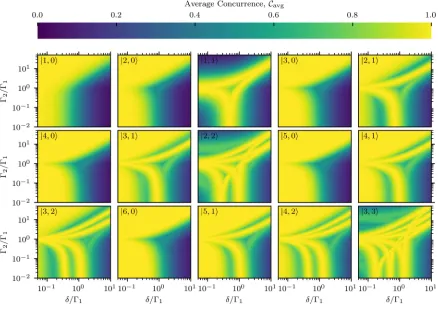
In Fig.1 we plot the average concurrence as a function of the emitter properties, Γ1, Γ2, andδ, for up to 6 photons.

[1] W. K. Wootters,Phys. Rev. Lett.80, 2245 (1998).

[2] M. A. Nielsen and I. Chuang, “Quantum computation and quantum information,” (2002). [3] C. K. Hong, Z. Y. Ou, and L. Mandel,Phys. Rev. Lett.59, 2044 (1987).