Robust Converter Control Design under Time-Delay Uncertainty

This is a repository copy of

Robust Converter Control Design under Time-Delay

Uncertainty

.

White Rose Research Online URL for this paper:

http://eprints.whiterose.ac.uk/146458/

Version: Accepted Version

Proceedings Paper:

Flores, DR, Markovic, U, Aristidou, P orcid.org/0000-0003-4429-0225 et al. (1 more author)

(2019) Robust Converter Control Design under Time-Delay Uncertainty. In: Proceedings of

the 2019 IEEE PowerTech conference. IEEE PowerTech 2019, 23-27 Jun 2019, Milan,

Italy. IEEE . ISBN 9781538647226

https://doi.org/10.1109/PTC.2019.8810516

This conference paper is protected by copyright. Uploaded in accordance with the

publisher's self-archiving policy.

eprints@whiterose.ac.uk https://eprints.whiterose.ac.uk/ Reuse

Items deposited in White Rose Research Online are protected by copyright, with all rights reserved unless indicated otherwise. They may be downloaded and/or printed for private study, or other acts as permitted by national copyright laws. The publisher or other rights holders may allow further reproduction and re-use of the full text version. This is indicated by the licence information on the White Rose Research Online record for the item.

Takedown

If you consider content in White Rose Research Online to be in breach of UK law, please notify us by

Robust Converter Control Design under Time-Delay

Uncertainty

David Rodriguez Flores

, Uros Markovic

, Petros Aristidou

, Gabriela Hug

§_{School of Electronic and Electrical Engineering, University of Leeds, Leeds LS2 9JT, UK}

Emails: roddavid@student.ethz.ch,{markovic, hug}@eeh.ee.ethz.ch, p.aristidou@leeds.ac.uk

Abstract—This paper deals with the converter control design under time delay uncertainty in power systems with high share of converter-based generation. Two approaches for time delay modeling are proposed using linear fractional transformations and linear parameter-varying systems, respectively. Subsequently, two output-feedback synthesis methods are implemented based on H∞ control theory, and formulated using linear matrix

inequalities: (i) a norm-bounded parametricH∞controller; and

(ii) a gain-scheduledH∞control. These robust control principles

are then employed to improve the performance of Voltage Source Converters (VSCs) under varying measurement delays. Three novel control strategies are proposed in order to redesign the conventional inner control loop and improve converter perfor-mance when dealing with measurement uncertainty. Finally, the controllers are integrated into a state-of-the-art VSC model and compared using time-domain simulations.

Index Terms—low-inertia systems, time delay, voltage source converter (VSC), linear fractional transformation (LFT), linear parameter-varying (LPV) system, robust stability, H∞control

I. INTRODUCTION

Conventional synchronous machines are being gradually replaced by renewable energy sources, interfaced to the grid through power electronic devices. The loss of traditional gen-erators comes along with the decrease in total rotational inertia of the system, thus affecting the system stability margins [1]. This problem has so far been dealt with through advanced converter AC-side control schemes, such as the virtual syn-chronous machine [2], machine matching [3] and dispacthable virtual oscillator control [4]. However, all of the proposed approaches involve local signal measurements, which are often subjective to time delays.

The subject of local time delay is often ignored in the area of power system control due to large time constants of the associ-ated machine regulators. Nonetheless, with shorter timescales, characteristic of low-inertia systems, the impact of local converter measurements might play an important role in the overall system stability. Different approaches for time-delay modeling have previously been investigated in [5], concluding that the Pad´e approximation and Chebyshev discretization scheme prevail as the most efficient methods. However, the focus was set solely on constant measurement delays with no uncertainty. A probabilistic approach for modelling the delays

This project has received funding from theEuropean Union’s Horizon 2020 research and innovation programmeunder grant agreement No 691800. This paper reflects only the authors’ views and the European Commission is not responsible for any use that may be made of the information it contains.

as a random variable and employing Monte Carlo simulations was used in [6], while [7] proposes a use of Lyapunov functions for deriving the delay-dependent stability criteria. The studies in [8] and [9] employ classical H∞ methods to deal with fixed delays, and [10] suggests a parameter-dependent H∞ gain-scheduling for delays within a certain tolerance. Other approaches in the literature consider a use of Smith predictors [11], adaptive control schemes [12] and lead-lag compensators [13]. Nonetheless, all aforementioned studies focus on conventional power systems and the underly-ing delays in wide-area measurements. While some concerns regarding the impact of local converter delays in low-inertia systems have already been raised in [14], it was done for a simplistic system without considering the delay uncertainty.

The contribution of this work is three-fold. First, we propose two ways of modelling the delay uncertainty and incorporating it into the Robust Control (RC) design. Moreover, two different output-feedback H∞ controllers are employed, each using a different delay uncertainty model, and compared under different measurement delay conditions. Finally, three novel RC strategies for redesigning the conventional Voltage Source Converter (VSC) control scheme are introduced, and analyzed using H∞-based techniques.

The remainder of the paper is structured as follows. In Sec-tion II the necessary RC principles along with the modelling of uncertain time delays are presented. The state-of-the-art converter control scheme and the novel robust controllers are described in Section III. Section IV showcases the detailed time-domain simulation results of the proposed control designs and compares their respective performances. Finally, Section V draws the main conclusions and discusses the outlook of the study.

II. RC PRINCIPLES UNDERTIME-DELAYUNCERTAINTY

A. Time Delay Modelling

We assume a real parametric uncertainty, and model the time delays in two different ways: (i) as a Linear Fractional Transformation (LFT); and (ii) as a Linear Parameter-Varying (LPV) system. In both cases the delays are modelled as exponential functions F(s) = e−τds

in the Laplace domain and are approximated using a first-order Pad´e approximation of the form:

F(s) =e−τds

≈ 1− 1 2τds

1 +1 2τds

1

τd

2

w 2

s z

w1 z1

− −

(a)

M

w1 z1

δt

yd

ud

(b)

ˆ

M(s)

w z

δt

yd

ud

(c)

Fig. 1: Equivalent representation of the delay function F(s): (a) control block scheme; (b) LFT formulation of the delay block τ−1

d ; (c) LFT formulation of the delay function F(s).

1) Time Delay as an LFT: The relation between the original signalw and its delayed counterpartz can be expressed as

z=F(s)w _7−→ z=−w+ 2

τds

(w₋z) (2)

which corresponds to the block diagram in Fig. 1a. The time delay parameter τd changes within a 1-dimensional polytope

[τ_d, τd]. By defining a = 1₂(τd+τd), b = 1₂(τd−τd) and

δt ∈ [−1,1], one can formulate such polytope asτd=a+bδt.

Therefore, the time-delay blockτ−1

d can be represented as an

upper LFT of the form Fu(M, δt)shown in Fig. 1b, with

M =

−ba−1 _a−1 −ba−1 _a−1

(3)

Substituting Fu(M, δt) in Fig. 1a and performing a set of

mathematical transformations yields the final LFT form de-picted in Fig. 1c, equivalent to the initial delay functionF(s), where

ˆ

M =

_ˆ

M11 Mˆ12

ˆ

M21 Mˆ22

= 1

−as+ 2b

as+b −2

2bs −s

(4)

2) Time Delay as an LPV function: Let us consider a delayed-input system without the controller. Based on the Pad´e approximation from (1), the following state-space representa-tion of the delay can be derived:

˙

xd=−

2

τd

xd+

4

τd

ud

yd=xd−ud

(5)

where ud and yd are the delayed input and output of the

system, and xd is the internal delay state. Substitutingq for

τ−1

d yields

Ad(q) Bd(q)

Cd(q) Dd(q)

=

−2q 4q

1 −1

(6)

The system in (6) can be rewritten as an affine parameter-dependent system, with the state-space matrices of the delay described as affine functions of the parameter q:

Ad(q) Bd(q)

Cd(q) Dd(q)

=

Ad0+qAd1 Bd0+qBd1

Cd0+qCd1 Dd0+qDd1

(7)

P

w z

∆

K

y∆

u∆

y u

(a)

P(., q)

w z

K(., q)

q(t)

y u

(b)

Fig. 2: General control plant: (a) LFT general plant. (b) LPV general plant.

B. _H∞ Control Design

This section elaborates on the principles ofH∞control. For the generic linear system described in (8), the H∞ norm is the maximum gain of the transfer function from exogenous inputs w to exogenous outputs z over all frequencies and input directions [15]. When designing H∞ controllers the system is rearranged into a so-called general control form illustrated in Fig. 2, whereP(s),K(s)and∆are the transfer functions of the plant, controller and uncertainty respectively; the uncertainty transfer function is not needed for the purposes of LPV system design. Therefore, without considering the uncertainty, letP(s)be of the following form:

˙

x=Ax+B1w+B2u

z=C1x+D11w+D12u

y=C2x+D21w+D22u

(8)

withubeing the control input andythe control measurement. TheH∞problem involves designing a controller that stabilizes the closed loop system and results in

Twz(s)_∞< γ (9)

for a given γ. Depending on the employed control synthesis method, the closed-loop system will also guarantee a degree of robustness against model uncertainty.

In order to shape the sensitivity function S(s) and com-plementary sensitivity function K(s)S(s) of the closed-loop system, and achieve the desired robustness and performance targets, a mixed-sensitivity H∞ design depicted in Fig. 3 is often used, which minimizes

W1(s)S(s)

W2K(s)S(s)

∞

(10)

The weight transfer functionW1(s)is usually a low-pass filter with the purpose of improving the output disturbance rejection or reference tracking, whereasW2(s)is a high-pass filter used for minimizing the control effort at high frequencies [15]. The mixed-sensitivity design is then solved by computing the augmented plant P(s) from the open-loop transfer function

G(s)and aforementioned weighting functions.

W1

W2

G

z1

z2

w

K e

−

y u

y′

Augmented plantP

Fig. 3: Mixed sensitivity_H∞ design.

uncertainty range and can be determined either through the structural singular value µ for LFT systems [15], or via a parameter-dependent Lyapunov function in the case of an LPV system [17]. Quadratic stability, on the other hand, is a fundamentally stronger concept of stability since it guarantees robust stability, as well as the resilience to arbitrary fast parameter changes [18]. However, it is also more conservative due to a single Lyapunov function being used for the whole uncertainty range.

C. Control Synthesis Methods

Two control synthesis methods are used, one for LFT modeling and another for LPV modeling. Both methods are defined using Linear Matrix Inequalities (LMIs) and are based on the concept of quadratic stability [18], [19]. Additional constraints are specified to place the poles of the closed-loop system in a specific region of the left-half plane in order to ensure the prescribed damping ratio requirements [20]. Both control synthesis problems are solved in MATLAB using the Yalmip interface [21] and SeDuMi/SDPT3 solvers [22], [23].

1) _H∞ Control for Norm-Bounded Parametric Systems: We aim to solve the H∞ performance problem of the form:

kHwzk∞<1 ,∀ k∆k2≤1 (11) which is equivalent to the robust stability of the closed-loop system with a virtual norm-bounded uncertainty

∆P(s)(k∆Pk∞≤1)inserted between the disturbance dand the error e [18]. Therefore, the overall uncertainty becomes

diag(∆,∆P). A scaling matrix L = diag(I,

√

ℓI) can be subsequently introduced to reduce the conservatism of the small-gain method as follows:

L

1/2_H

zwL−1/2

_∞< γ (12)

whereL is permutable withdiag(∆,∆P).

The scaled _H∞ problem is solved if and only if there exist matrices X > 0, Y > 0, and L, J satisfying the following

conditions:

NT

X 0

0 Inw





AX+XAT _XCT

1 B1

C1X −γJ D11

BT

1 DT11 −γL





NX 0

0 Inw

<0

NT

Y 0

0 Inz





Y A+AT_{Y Y B}

1 CT1

BT

1Y −γL D11T

C1 D11 −γJ





NY 0

0 Inz

<0

X I

I Y

≥0

LJ=I

(13)

The last equalityLJ =Iis not convex, but the problem can be solved using theK-L iteration method proposed in [18].

2) Gain-Scheduled (GS) _H∞ Control for LPV Systems: This problem seeks a controller of the form:

˙

xk =Ak(q)xk+Bk(q)uk (14)

yk =Ck(q)xk+Dk(q)uk (15)

When the parameter vectorq(t)takes values in a boxB ∈Rn

withN= 2n_{corners, then the systemG(q)is confined within}

a matrix polytope defined by verticesG(θi). Given the convex

decomposition

q=

N

X

i=1

αiθi (16)

the controller state space can be written as

Ak(q) Bk(q)

Ck(q) Dk(q)

=

N

X

i=1

αi

Ak(θi) Bk(θi)

Ck(θi) Dk(θi)

(17)

Subsequently, the controller operating pointqis found through convex interpolation of the LTI vertex controllers:

Ki=

Ak(θi) Bk(θi)

Ck(θi) Dk(θi)

The gain-scheduling problem can be thus solved by solving the following LMI problem for symmetric matricesX andY:

N12 0

0 I

T 



A(θi)X+XAT_{(θi) XC}T

1(θi) B1(θi)

C1(θi) −γI D11(θi)

BT

1 D11T(θi) −γI





N12 0

0 I

<0

N21 0

0 I





AT_{(θi)Y +Y A Y B}

1(θi) C1T(θi)

BT

1(θi)Y −γI DT11(θi)

C1(θi) D11(θi) −γI





N21 0

0 I

<0

X I

I Y

≥0

(18)

with N12 and N21 denoting the bases of the null spaces of

(B2T, D12T)and(C2, D21)respectively. The optimal controller

K is derived fromX andY.

III. VSC CONTROLDESIGN

A. VSC Control Scheme

We consider a state-of-the-art VSC control scheme previ-ously described in [24], where the outer control loop consists of droop-based active and reactive power controllers providing the output voltage angle and magnitude reference by adjusting the predefined setpoints (x∗

Cdc vdc

v_t Grid

dq

abc

dq abc

idq_g τ Power

Calculation Unit

edq gτ

Phase Locked

Loop

SRF Voltage Controller

SRF Current Controller

PWM Reactive

Power Controller

Active Power Controller

Virtual Impedance

Block

q∗

c

v∗

c

p∗

c

ω0

h edq

gτ,i

dq gτ i

θc

Rt Lt

v_m idq

sτ

Rf

Lf

Cf

iabc g

eabc g

¯

i_s v_¯m m

qc

pc

ωc vdc

¯ v

vc

ωpll

Inner control loop Outer control loop

i_t

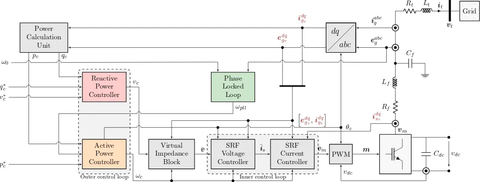
Fig. 4: General configuration of the implemented VSC control structure. The delayed measurements are denoted in red.

(vc∠θc)is passed through a virtual impedance block, as well

as the inner control loop consisting of cascaded voltage and current controllers. The output is combined with the DC-side voltage in order to generate the modulation signal m. In order to detect the system frequency at the connection terminal, a synchronization unit in the form of a phased-locked loop is included in the model. Furthermore, the time delays are imposed onto the local measurement signals (e_g,i_g,i_s), denoted with a subscriptτ in Fig. 4. Since the measurements are obtained from a single device, we assume the same time delay for all signals. The complete mathematical model consists of 15 states, with inclusion of the filter current and voltage dynamics, and is implemented in a rotating (dq) -frame and per unit. More details on the overall converter con-trol structure, employed parametrization, potential operation modes and respective transient properties can be found in [24].

B. Robust Control Design

The vulnerability of the system to measurement delays is first evaluated through small-signal stability for a wide range of time delays. The eigenvalue spectrum illustrated in Fig. 5 indicates a critical delay of τˆd ≈ 314µs, and suggests the

presence of 4 critical modes. According to the participation factor analysis, the states with the highest participation in those modes are the filter current and voltage (i_s,e_{g), with} the former having the highest impact. Hence, the inner control loop can be considered the main cause of instability.

The traditional inner control design consists of a cascade of PI controllers and feed-forward loops, as follows:

¯i_s=

Kpv+

Kiv

s

(¯v₋e_{g) +jxf}e_g+Ki

fig (19)

¯

v(0)

m =

Kpi+

Kii

s

∆i_s

τ +jxfisτ +K

v

fegτ (20)

where ∆i_s

τ = ¯is−isτ, the subscriptsp,i andf denote the

respective proportional, integral and feed-forward gains, and the superscriptsvandirefer to the voltage and current control.

−4,000 −3,000 −2,000 −1,000 0

−1

−0.5 0 0.5

1 ·10

4

ℜ(λ)

ℑ

(

λ

)

τd= 50µs

τd= 100µs

τd= 150µs

τd= 200µs

τd= 250µs

τd= 300µs

τd= 350µs

Fig. 5: Root loci spectrum around the imaginary axis computed using the Pad´e approximation.

In order to improve the converter performance under mea-surement delay, we propose three novel control strategies:

¯

v(1)

m =

K_pi+K

i i

s

∆i_s

τ+jxfisτ +K

v

fegτ − K1(∆egτ)

¯

v(2)

m =

Kpi+

Ki i

s

∆i_g

τ +jxfigτ+K

v

fegτ − K2(∆egτ)

¯

v(3)

m =K3(¯v−egτ) (21)

The first two approaches depicted in Fig. 6a consist of adding an additional damping termK1,2 to the current control based on the deviation of the voltage across the filter capacitor from its nominal value(∆e_g

τ). The latter design also uses different

current input measurement, replacing the switching currenti_s

τ

with the grid current inputi_g

τ in order to reduce the control

SRF Voltage Controller ¯

v

θc

SRF Current Controller h

edq gτ,i

dq gτ i

idq

sτ

K1,2

ωc

∆edq gτ

¯ v_m ¯i_s

Inner control loop

(a)

K3 ¯

v

θc e dq gτ

K1,2

¯ v_m

Inner control loop

(b)

Fig. 6: Control design strategies: (a) robust active damping control (K1,K2); (b) uniform robust inner control(K3).

the need for any current measurement input, as described in Fig. 6b, thus providing a lower controller order.

Two H∞ output feedback controllers are implemented for each design: an LFT norm-bounded controller and a GS controller, previously described in Section II-C. The weighting transfer functions used in the mixed-sensitivity design of K1 and K2 are: W1(s) = 0.5_ss₊₅+500, W2(s) = 1. Since the controller K3 tracks the voltage output of the converter, the weights are chosen such that a good integral control performance in time domain is achieved. The bandwidth of the controller is therefore set to1000rad/s, resulting in the fol-lowing weighting functions: W1(s) = 0.5_ss₊₀+1000_.1 ,W2(s) = 1.

IV. RESULTS

An overview of the stability performance obtained from the proposed control designs is presented in Table I. We can observe that the range of time delays for which the robust and quadratic stability are guaranteed, as well as the order of the controllers, vary significantly between different control approaches. As described previously in Section II, the em-phasis is put on quadratic stability, as it allows for arbitrarily fast variation of measurement delays. Understandably,K3has the lowest order due to removal of the current measurements from the control input. It also provides a drastically larger stability range, both under LFT and GS implementation. This is a consequence of its conceptually superior design, which eliminates a majority of the state feedback sensitive to time delays. Moreover, the GS approach appears to be the more robust of the two, with the respective critical delayτˆdreaching

millisecond range.

We now investigate the converter response to a 10 % step increase in active power setpoint, and evaluate its reference tracking capability under different measurement delay prop-erties. For this purpose, detailed time-domain simulations in

TABLE I: Stability performance of different control designs.

Control Order QS Range RS Range K1,LFT 21 [0−370]µs [0−420]µs

K1,GS 21 [0−750]µs [0−750]µs

K2,LFT 19 [0−400]µs [0−660]µs

K2,GS 19 [0−2]ms [0−2]ms

K3,LFT 15 [0−900]µs [0−1]ms

K3,GS 15 [0−20]ms [0−50]ms

0.5 0.55 0.6

pc

[p

.u

.] K1,LFT

K1,GS

K2,LFT

K2,GS

K3,LFT

K3,GS

0.5 0.55 0.6

pc

[p

.u

.] K1,LFT

K1,GS

K2,LFT

K2,GS

K3,LFT

K3,GS

0 0.5 1 1.5 2

0.5 0.55 0.6

t[s]

pc

[p

.u

.] K1,LFT

K1,GS

K2,LFT

K2,GS

K3,LFT

K3,GS

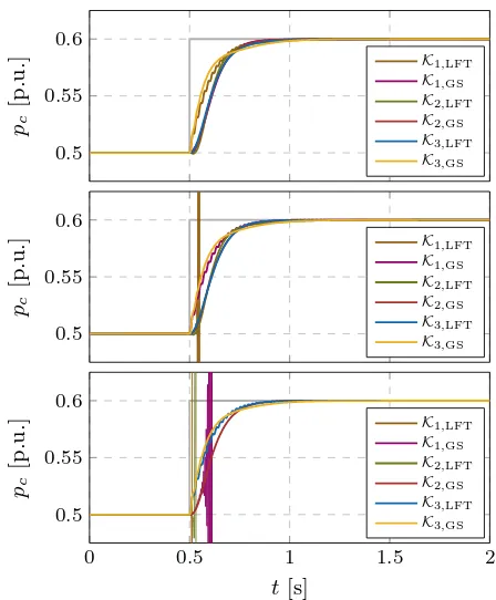
Fig. 7: Response to a step-change in active power setpoint under constant time delay for different inner control designs: (i)τd= 150µs; (ii)τd= 500µs; (iii)τd= 1ms;.

MATLAB Simulink have been used. A focus is first set on constant delays in a range of [150−1000]µs and the results are presented in Fig. 7. Under a reasonably small delay of150µs all controllers achieve good performance, with controller K3,GS having the best overall response due to a combination of its reduced system order and gain scheduling design. Nonetheless, such level of delay could be withstood by a conventional inner control, which is not the case in the next two scenarios. Forτd∈[500,1000]µs we observe that certain

control designs are unstable, which can be justified by their insufficient robust stability range in Table I. More precisely, K1,LFT has a critical delay threshold below 500µs, whereas K1,GSandK2,LFTcannot withstand a1ms measurement delay. Accounting for time delay variability, a quadratic stability aspect becomes more relevant, as it ensures resilience to fast changes in the delay signal. Therefore, we consider a delay varying as a sinusoidal function of the formτd=Td|sin (ωt)|,

with Td = 1ms. The converter power response illustrated

in Fig. 8 indicates that only the controllers with an accept-able quadratic stability range can tolerate such an oscillatory delay nature. As a result, the LFT designs of K1 and K2 underperform wheneverτd goes drastically above370µs and

400µs, respectively. A similar characteristic is noticeable for K3,LFT, withˆτd= 900µs being slightly below the delay peak.

0 0.2 0.4 0.6 0.8 1

τd

[m

s]

0 0.5 1 1.5 2

0.5 0.55 0.6

t[s]

pc

[p

.u

.] K1,LFT

K1,GS

K2,LFT

K2,GS

K3,LFT

K3,GS

Fig. 8: Response to a step-change in active power setpoint under varying time delay for different inner control designs: (i) varying time delay signal; (ii) converter power output.

stability ranges.

It can be concluded that the K3 concept clearly shows the best performance, independent of the control synthesis method. It completely replaces the inner control loop, reduces the overall control order and ensures excellent robustness to any type of measurement delay. On the other hand, theK1and K2configurations have an inherent disadvantage of adding an extra controller to the existing system and increasing complex-ity. Furthermore,K1achieves only a minor improvement to the original design, whereas K2, although significantly better, is still suboptimal compared to the uniform structure of K3.

V. CONCLUSION

In this paper, the robust control design under time delay uncertainty in power systems with a high share of converter-based generation is investigated. Two ways of time delay modeling are presented, and subsequently used for developing two output-feedback synthesis methods based onH∞ control theory. In order to improve the resilience of VSCs to varying delays in local measurement, three novel control strategies are proposed and combined with each of the two synthesis methods. A redesign of the conventional inner control loop is suggested, which improves converter performance when dealing with measurement uncertainty. It was found that the uniform controller performs the best and guarantees quadratic stability for a wide range of time delays. Furthermore, the gain-scheduling synthesis appeared to be the more practical approach of the two. Future work will focus on large-scale systems, as well as the impact of signal delay in wide-area measurements involved in centralized power system control schemes.

REFERENCES

[1] A. Ulbig, T. S. Borsche, and G. Andersson, “Impact of low rotational inertia on power system stability and operation,” IFAC Proceedings Volumes, vol. 47, no. 3, pp. 7290 – 7297, 2014.

[2] J. Driesen and K. Visscher, “Virtual synchronous generators,” in2008 IEEE Power and Energy Society General Meeting - Conversion and Delivery of Electrical Energy in the 21st Century, July 2008. [3] C. Arghir, T. Jouini, and F. D¨orfler, “Grid-forming control for power

converters based on matching of synchronous machines,” Automatica, vol. 95, pp. 273 – 282, 2018.

[4] M. Colombino, D. Groß, J.-S. Brouillon, and F. D¨orfler, “Global phase and magnitude synchronization of coupled oscillators with applica-tion to the control of grid-forming power inverters,” arXiv preprint arXiv:1710.00694, 2017.

[5] F. Milano, “Small-signal stability analysis of large power systems with inclusion of multiple delays,” IEEE Transactions on Power Systems, vol. 31, no. 4, pp. 3257–3266, 2016.

[6] S. Ayasun and C. O. Nwankpa, “Probability of small-signal stability of power systems in the presence of communication delays,” in Elec-trical and Electronics Engineering, 2009. ELECO 2009. International Conference on. IEEE, 2009, pp. I–70.

[7] T. Li, M. Wu, and Y. He, “Lyapunov-Krasovskii functional based power system stability analysis in environment of wams,”Journal of Central South University of Technology, vol. 17, no. 4, pp. 801–806, 2010. [8] D. Ke, C. Chung, and Y. Xue, “An eigenstructure-based performance

index and its application to control design for damping inter-area oscillations in power systems,”IEEE Transactions on Power Systems, vol. 26, no. 4, pp. 2371–2380, 2011.

[9] R. Shah, N. Mithulananthan, K. Y. Lee et al., “Large-scale pv plant with a robust controller considering power oscillation damping,”IEEE Transactions on Energy Conversion, vol. 28, no. 1, pp. 106–116, 2013. [10] H. Wu, K. S. Tsakalis, and G. T. Heydt, “Evaluation of time delay effects to wide-area power system stabilizer design,”IEEE Transactions on Power Systems, vol. 19, no. 4, pp. 1935–1941, Nov 2004. [11] T. Zabaiou, L.-A. Dessaint, F.-A. Okou, and R. Grondin, “Wide-area

coordinating control of svcs and synchronous generators with signal transmission delay compensation,” inPower and Energy Society General Meeting, 2010 IEEE. IEEE, 2010, pp. 1–9.

[12] B. Chaudhuri, R. Majumder, and B. C. Pal, “Wide-area measurement-based stabilizing control of power system considering signal transmis-sion delay,” IEEE Transactions on Power Systems, vol. 19, no. 4, pp. 1971–1979, 2004.

[13] P. Zhang, D. Yang, K. Chan, and G. Cai, “Adaptive wide-area damp-ing control scheme with stochastic subspace identification and signal time delay compensation,”IET generation, transmission & distribution, vol. 6, no. 9, pp. 844–852, 2012.

[14] U. Markovic, P. Aristidou, and G. Hug, “Stability performance of power electronic deviceswith time delays,” in2017 IEEE Manchester PowerTech. IEEE, 2017.

[15] S. Skogestad and I. Postlethwaite, Multivariable feedback control: analysis and design. Wiley New York, 2007, vol. 2.

[16] B. Barmish, “Stabilization of uncertain systems via linear control,”IEEE Transactions on Automatic Control, vol. 28, no. 8, pp. 848–850, 1983. [17] W. Haddad and D. Bernstein, “Parameter-dependent lyapunov functions, constant real parameter uncertainty, and the popov criterion in robust analysis and synthesis. 1,” inDecision and Control, 1991., Proceedings of the 30th IEEE Conference on. IEEE, 1991, pp. 2274–2279. [18] K.-Z. Liu and Y. Yao,Robust control: theory and applications. John

Wiley & Sons, 2016.

[19] P. Apkarian and P. Gahinet, “A convex characterization of gain-scheduledH∞controllers,”IEEE Transactions on Automatic Control,

vol. 40, no. 5, pp. 853–864, May 1995.

[20] M. Chilali, P. Gahinet, and P. Apkarian, “Robust pole placement in lmi regions,”IEEE transactions on Automatic Control, vol. 44, no. 12, pp. 2257–2270, 1999.

[21] J. Lofberg, “Yalmip: A toolbox for modeling and optimization in matlab,” in Computer Aided Control Systems Design, 2004 IEEE In-ternational Symposium on. IEEE, 2004, pp. 284–289.

[22] J. F. Sturm, “Using sedumi 1.02, a matlab toolbox for optimization over symmetric cones,”Optimization methods and software, vol. 11, no. 1-4, pp. 625–653, 1999.

[23] K.-C. Toh, M. J. Todd, and R. H. T¨ut¨unc¨u, “Sdpt3a matlab software package for semidefinite programming, version 1.3,”Optimization meth-ods and software, vol. 11, no. 1-4, pp. 545–581, 1999.