Essays in international finance

(1)

City, University of London Institutional Repository

Citation

:

Passari, Evgenia (2013). Essays in international finance. (Unpublished Doctoral thesis, City University London)

This is the unspecified version of the paper.

This version of the publication may differ from the final published

version.

Permanent repository link:

http://openaccess.city.ac.uk/3062/

Link to published version

:

Copyright and reuse:

City Research Online aims to make research

outputs of City, University of London available to a wider audience.

Copyright and Moral Rights remain with the author(s) and/or copyright

holders. URLs from City Research Online may be freely distributed and

linked to.

City Research Online: http://openaccess.city.ac.uk/ [email protected]

(2)

by Evgenia Passari

A thesis submitted in partial ful…lment

of the requirements for the degree of

Doctor of Philosophy in Finance

Cass Business School

City University

(3)

List of Tables 4

List of Figures 6

Introduction 11

Chapter 1. In Quest for a Robust Model of the Exchange Rate: A Collective

Approach 19

1.1. Introduction 19

1.2. Selective Literature Review 23

1.3. The Models 28

1.4. Empirical Results 34

1.5. Economic Value 40

1.6. Conclusion 42

Appendix:In-Sample Estimation of the Models 45

Appendix Tables 48

Tables 58

Figures 62

Chapter 2. Purchasing Power Parity in Tradable Goods 73

2.2. The LOP and Price Indices 74

(4)

2.6. Conclusion and implications 105

Appendix: TAR modeling 106

Figures 108

Chapter 3. Commodity Currencies Revisited 116

3.2. Commodities and the Exchange Rate: Selective Literature Review 119 3.3. Framework for the Commodity Currency Strategy 121

3.4. Data and Currency Portfolios 124

3.5. Comparing the Commodity Currency Strategy to Carry Trade 125

3.6. Empirical Results 128

3.7. Discussion 133

3.8. Robustness 134

3.9. Conclusion 136

Tables 138

Figures 157

Chapter 4. Concluding remarks 159

(5)

1.1 Out-of-Sample Forecasting Ability: Developed Markets 58 1.2 Out-of-Sample Forecasting Ability: Emerging Markets 59 1.3 Out-of-Sample Forecasting Ability: Combined Model, Developed and

Emerging Markets 60

1.4 Calculation of Performance Fees 61

2.1 TAR estimation results: UK, Japan and Germany 107

3.1 Countries and Commodities 138

3.2 Currency Beta Rankings versus the USD and GBP 139 3.3 Descriptive Statistics: Commodity Strategy, Spot Returns 140 3.4 Descriptive Statistics: Commodity Strategy, Excess Returns 141 3.5 Descriptive Statistics: Carry Trade, Spot Returns 142 3.6 Descriptive Statistics: Carry Trade, Excess Returns 143 3.7 Correlation of Commodity Strategy and Carry Trade Returns 144 3.8 Commodity Strategy and Carry Trade: Double Sorts 145

3.9 Principal Components 146

(6)

3.15Descriptive Statistics: Commodity Strategy, Excess and Net Excess

(7)

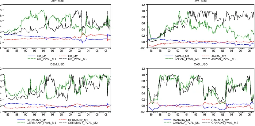
1.1 Developed Markets panel: Coe¢ cients and p-values for the MA model at

the 1-month horizon. 62

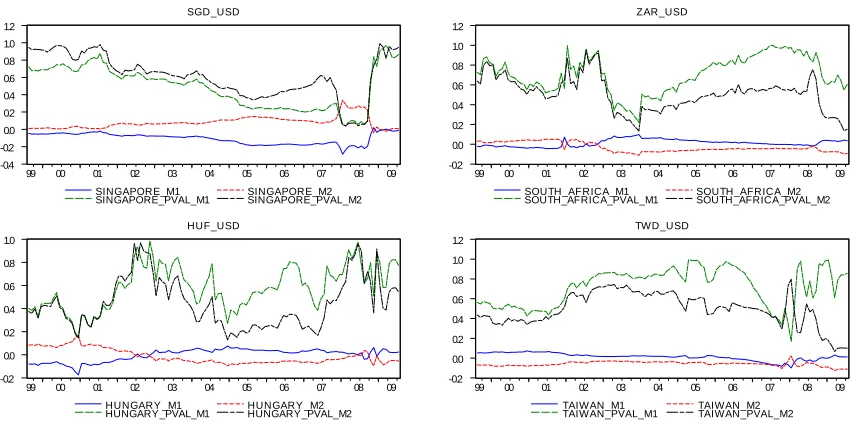
1.2 Emerging Markets panel: Coe¢ cients and p-values for the MA model at

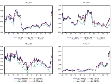
1.3 Rolling Regression Results for the Developed Markets panel: RMSPEs at

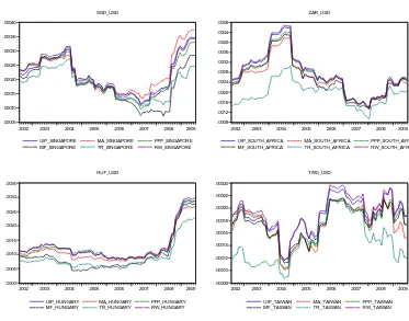
1.4 Rolling Regression Results for the Emerging Markets panel: RMSPEs at

the 1-year horizon. 66

1.9 Developed Markets panel: Coe¢ cients for the Combined model at the

1-month horizon. 70

1.10Developed Markets panel: P-values for the Combined model at the

(8)

2.1 Logarithm of GBP/USD Real Exchange Rate, 1791-2010. 108 2.2 GBP/USD: Real Exchange Rates Calculated Using Di¤erent Price Indices

(1973-2010). 109

2.3 JPY/USD: Real Exchange Rates Calculated Using Di¤erent Price Indices

(1973-2010). 110

2.4 DEM-EUR/USD: Real Exchange Rates Calculated Using Di¤erent Price

Indices (1991-2010). 111

2.5 Real Exchange Rates against the USD (1973-2010). 112 2.6 GBP/USD Nominal Exchange Rate versus GBP/USD PPP Spot Rate

(OECD Data), 1973-2010. 113

2.7 JPY/USD Nominal Exchange Rate versus JPY/USD PPP Spot Rate

(OECD Data), 1973-2010. 114

2.8 DEM-EUR/USD Nominal Exchange Rate versus DEM-EUR/USD PPP

Spot Rate (OECD Data), 1973-2010. 115

(9)

I am hugely indebted to my supervisors Lucio Sarno and Ian Marsh for their constant mentorship and support during the last four years as well as to the Fi-nance Group at Cass Business School for the numerous valuable comments and discussions. I am also obliged to Ilias Tsiakas for his guidance.

Furthermore, I am grateful to Hélène Rey and Elias Papaioannou for being a great source of inspiration and to the Economics Faculty at London Business School, where this thesis was partly written. I would also like to thank Thomas Stolper and all my colleagues at Goldman Sachs for their warm welcome during my summer appointment.

I am grateful to my parents Aristea and Ioannis, and to my brother Stelios. John deserves a very special mention for his patience, help and encouragement. I also thank Konstantina and Despoina for their support.

Additionally, I would like to thank for their help and constructive comments: Giorgio Valente, Ana-Maria Fuertes, Giovanni Urga, Roy Batchelor, Richard Payne, Kate Phylaktis, Simon Haylay, Michael Moore, Robert Vigfusson, Lorenzo Trapani, Pasquale Della Corte, Øystein Børsum, Jerry Coakley, Tom Fearnley, Lawrence O¢ cer, Vania Stavrakena, Deepa Dhume Datta, Gino Cenedese, Cheng Yan, Bar-bara Ulloa, Chiara Banti, Kaizad Doctor, Ekaterina Ipatova, Evangelos Aspiotis, Chris Lega, and the seminar participants at the 2012 International Conference on Macroeconomic Analysis and International Finance at the University of Crete, the 2012 International FEBS Conference at ESPC Europe Business School and the 2011 Annual Conference of the Royal Economic Society at the Royal Holloway.

I am also thankful to my friends and colleagues at Cass Business School, War-wick Business School, and London Business School.

(10)

I declare that any material contained in this thesis has not been submitted for a degree to any other university. I further declare that the paper titled “Purchasing Power Parity in Tradable Goods”, drawn from Chapter Two of this thesis, is co-authored with Ian Marsh and Lucio Sarno and is published in the Handbook of Exchange Rates, edited by Jessica James, Ian W. Marsh, and Lucio Sarno. Finally, I grant powers of discretion to the City University Librarian to allow this thesis to be copied in whole or in part without further reference to me.

Evgenia Passari

(11)

the foreign exchange market. The …rst chapter assesses the predictive ability of a

com-prehensive set of empirical models of exchange rates, in addition to a standard technical

trading strategy, on monthly exchange-rate returns for four developed and four

emerg-ing countries across di¤erent horizons. I implement a rollemerg-ing window approach to the

estimation and forecasting of the models, and construct an encompassing forecast. I

also assess the economic value of the out-of-sample forecasting power of the empirical

models using a simple dynamic allocation strategy, and …nd three key results: (1) the

Taylor rule model consistently outperforms, economically and statistically, all the other

models at the 1-month horizon. (2) The technical rule has superior predictive power

over the random walk benchmark, across horizons, particularly for developed markets.

(3) There are statistical gains from an unrestricted combined forecasting model at the

1-month horizon. The second chapter constitutes a survey that focuses on

internation-ally tradable goods and services. Our motivation is that while excellent surveys exist

in the literature on this topic, they focus largely on broad baskets of prices and, most

commonly, on the consumer price index. We instead focus on the speci…c subset of the

relevant literature that analyses deviations from the LOP applied to individual goods

and services and speci…c sectors. The emphasis is hence on tradable items rather than

broad baskets that also include a substantial nontradable component. Speci…cally, the

objective is to distil the literature on the properties of deviations from the LOP applied

to internationally tradable goods or sectors. We conclude that a careful reading of the

literature suggests that this notion of PPP holds in the long run for a broad range of

tradable goods and services and for a broad set of currencies. In the third chapter, I

build a "commodity currency strategy" for exchange rate forecasting that conditions on

changes in the global prices of commodity indices. The risk-return pro…le of this

strat-egy reveals that the predictive ability of commodity prices for the exchange rate appears

to be signi…cant, and the returns appear to be uncorrelated to popular exchange rate

strategies such as the carry trade and currency momentum. The market factor captures

more than 70% of the cross-sectional returns of the proposed strategy and suggests a

negative relation between equity returns and currency returns that are driven by

(12)

The present thesis comprises three essays in international …nance, with a focus on the foreign exchange market. The …rst chapter assesses the predictive ability of a comprehensive set of empirical models of exchange rates, in addition to a standard technical trading strategy, on monthly exchange-rate returns for four developed and four emerging countries across di¤erent horizons. My motivation is the large gap that exists between the models used by academics and those adopted by market practitioners. The former tend to employ long run equilibrium equations based on fundamental variables and use standard distribution theory in their modeling approach. In contrast, the majority of market practitioners adopt chartism, which is essentially the use of technical trading rules that lack a theoretical foundation. However, none of these two competing approaches has managed, so far, to provide a model of exchange rate behaviour that performs well at di¤erent frequencies. The aim of this chapter is to provide a statistical and economic investigation of a comprehensive menu of fundamental models and a chartists’rule, across di¤erent forecast horizons, in an attempt to shed some light on this long-standing debate.

(13)

balance model and the more sophisticated new open economy models. More recent work carried by Molodtsova and Papell (2009) focuses on variants of the Taylor Rule model, testing the performance of speci…cations with richer dynamics and providing promising results. Finally, a strand of foreign exchange literature targets microstructural issues of the foreign exchange market in an attempt to rationalize the observed deviations from economic fundamentals. Nevertheless, there has not been a single theory that has managed to provide a fully satisfactory description of exchange rate dynamics, or present robust empirical success across horizons.

On the other hand, market practitioners tend to believe that exchange rate behaviour is, to some extent, predictable with simple rules. Their forecasting methods include technical trading rules, ad hoc techniques and patterns, such as moving average crossovers, oscillators and range breakouts. The majority of aca-demics has long considered these techniques of no value as they lack intuition and objectivity. Interestingly enough, the empirical evidence suggests that technical analysis not only shows no tendency to disappear in the long run but is indeed pro…table (Menkho¤ and Taylor, 2007). Besides, survey papers report that the vast majority of foreign exchange market participants use chartism at the short-term horizon, while fundamentals are considered more important in the long run, citing the work of Taylor and Allen (1992), Cheung and Chinn (2001), Gehrig and Menkho¤ (2004) and Menkho¤ (2010). Given that the purpose of this study is to explore the dynamics of the foreign exchange market, a market that is highly dom-inated by market makers (mainly commercial and investment banks), one tends to think that the incorporation of the practitioners’view into the model is a poten-tially meaningful endeavour.

(14)

In the present chapter, I attempt to provide a comprehensive investigation of a large menu of standard models for the exchange rate, including a conventional Moving Average (MA) rule, a rich speci…cation of the Taylor Rule model and a forecast encompassing of all the models, on monthly exchange-rate returns, for four developed and four emerging countries across di¤erent horizons. For this purpose, I implement a rolling window approach to the estimation and forecasting of the models, along with a standard, full sample estimation. The performance of the combined strategies, in- and out-of-sample, constitutes one of the main contributions of this chapter and o¤ers a novel way to carry out model evaluation both statistically and economically.

I further examine whether the weight given to chartism relative to fundamen-tal analysis decreases with the forecast horizon as it has been well documented by both survey data papers and empirical studies (Menkho¤ and Taylor, 2007). I also explore how the relative importance of the MA model evolves over time and investigate whether technical analysis tends to matter more for emerging mar-ket currencies, as the documented pro…tability of volatile currencies potentially indicates that chartism has a greater impact on developing markets relative to developed markets.

Finally, an important contribution is the assessment of the economic value of the out-of-sample forecasting power of the empirical models using a simple dynamic allocation strategy, which entails the computation of out-of-sample performance fees (as in Della Corte, Sarno and Sestieri, 2010), originally proposed by Goet-zmann, Ingersoll, Spiegel and Welch (2007), an attractive measure that assumes neither a speci…c utility function nor a speci…c distribution of portfolio returns.

(15)

pro…tability of sophisticated technical trading rules, such as psychological barriers, and support and resistance levels. As a result, I do not build on the evidence documented by De Grauwe and Decupere (1992), and Osler (2000, 2003). Second, my work does not constitute a contribution on the extensive literature of forecast combination techniques. Instead, I focus on implementing a benchmark model of exchange rates. Finally, I do not and cannot make a statement on the e¢ ciency of the currency market.

To preview my results, I …nd that the Taylor rule model consistently outper-forms, economically and statistically, the interest rate parity, purchasing power parity, and monetary fundamental models as well as the technical trading strategy at the 1-month horizon. This is an important result that adds evidence on the performance of the model beyond the …ndings of Molodtsova and Papell (2009). I further maintain that the technical rule has superior predictive power over the random walk benchmark, across horizons, and document evidence of statistical gains from a forecast encompassing of the models at the 1-month horizon, …ndings that justify what practitioners do.

(16)

While several surveys exist on PPP, this chapter focuses mainly on internation-ally tradable goods and services, rather than broad baskets of goods and services that also include a substantial nontradable component. Speci…cally, the objective is to understand the properties of deviations from the LOP applied to interna-tionally tradable goods or sectors, on the basis of the existing empirical evidence published in the leading academic literature. To anticipate our conclusions, we show that a careful reading of the literature suggests that the LOP holds over long periods of time for the relevant tradable goods and services, and that adjustment occurs in a nonlinear fashion such that the larger the current deviation from parity the faster the adjustment towards parity in the future.

The core of the chapter focuses on the speci…c subset of the relevant literature that analyses deviations from the LOP applied to individual goods and services and speci…c sectors. The emphasis is therefore on tradable items. This literature, while less voluminous than the literature on PPP, is nevertheless substantial and it has not been summarized in a survey article to date. This is exactly the gap that this chapter …lls, with the ultimate goal to describe the current state of knowledge on the properties of deviations from the LOP, including the persistence of deviations from the LOP across currencies (the speed of reversion to the LOP), and the nature of the shocks.

The discussion of this chapter follows similar steps to the leading surveys on PPP, but with a more speci…c focus on internationally tradable goods and a speci…c description of some of the key studies that have best addressed this topic.

In the third chapter, I build a "commodity currency strategy" for the exchange rate that takes into account changes in the global prices of commodity indices.

(17)

ing the existence of a relationship but reporting limited predictability success. I deviate from this traditional approach motivated by two observations. First, so far it has yet to be established whether a currency investor could bene…t from the information embedded in commodity price changes; second, when it comes to the relationship dynamics, the forecasting framework renders the assessment of di¤erent variables and markets an arduous task.

In the present chapter, I examine the implications of the documented relation-ship between currencies and commodities for an investor’s currency allocation deci-sions. For this purpose, I build a country-speci…c commodity currency strategy by taking into account the countries’most important commodity imports and exports given a certain threshold. I further extend my country panel to include commodity importers as well as exporters in order to study whether this relationship holds for commodity currencies only. Throughout the empirical exercise, I employ trad-able commodity price indices in order to circumvent potential liquidity issues. I, then, study the risk-return pro…le of the proposed commodity currency strategy. In this way, I o¤er a di¤erent perspective in the debate regarding the dynamics between the countries’ exchange rate movements and the corresponding changes in the world price of commodity imports and exports.

In my empirical analysis I follow the recent literature (Lustig and Verdelhan (2007), Lustig, Roussanov, and Verdelhan (2011)) and allocate currencies into portfolios in accordance with the predictions of the proposed commodity currency strategy on a daily frequency. I construct …ve such portfolios. Going long in the

(18)

commodity portfolio. This strategy yields signi…cant unconditional spot excess re-turns, greater than 6% p.a., that appear to be uncorrelated to standard strategies such as the carry trade. Furthermore, these returns cannot be explained in a linear asset pricing framework (e.g. Ang, Hodrick, Xing, and Zhang (2006)) by measures of risk that have been found to fare well in the exchange rate literature such as global FX volatility risk and currency momentum; e.g. see Menkho¤, Sarno, Schmeling, and Schrimpf (2012a and b). Furthermore, I test whether standard risk factors can price the cross section of commodity portfolios.

The present chapter relates to two strands of the recent literature. First, my work contributes to the literature that investigates the relationship between ex-change rates and fundamentals and in particular, commodities. In line with this literature, I …nd a strong relationship between commodities and currencies; how-ever, my results are of a di¤erent nature as I focus on economic value instead of statistical predictability. Second, as in Lustig, Roussanov, and Verdelhan (2011), I cross-sectionally relate the commodity currency strategy returns to a set of risk factors.

(19)

currency behaviour.

The second set of my results relates to the determinants of the strategy’s suc-cess which are hard to precisely identify in an asset pricing framework. At the same time, the …ndings of the asset pricing exercise underline the complexity of dynamics that pertains to the examined relationship. For instance, although the equity market factor explains more than 70% of the cross-sectional returns of the commodity currency strategy, I …nd a negative relation between equity returns and currency returns that are driven by commodity price changes.

(20)

In Quest for a Robust Model of the Exchange Rate: A

Collective Approach

1.1. Introduction

A large gap exists between the models used by academics and those adopted by market practitioners. The former tend to employ long run equilibrium equations based on fundamental variables and use standard distribution theory in their mod-eling approach. In contrast, the majority of market practitioners adopt chartism, which is essentially the use of technical trading rules that lack a theoretical foun-dation. However, none of these two competing approaches has managed, so far, to provide a model of exchange rate behaviour that performs well at di¤erent frequen-cies. The aim of this chapter is to provide a statistical and economic investigation of a comprehensive menu of fundamental models and a chartists’rule, across dif-ferent forecast horizons, in an attempt to shed some light on this long-standing debate.

(21)

price monetary model, equilibrium and liquidity models, as well as the portfolio balance model and the more sophisticated new open economy models. More recent work carried by Molodtsova and Papell (2009) focuses on variants of the Taylor Rule model, testing the performance of speci…cations with richer dynamics and providing promising results. Finally, a strand of foreign exchange literature targets microstructural issues of the foreign exchange market in an attempt to rationalize the observed deviations from economic fundamentals. Nevertheless, there has not been a single theory that has managed to provide a fully satisfactory description of exchange rate dynamics, or present robust empirical success across horizons.

On the other hand, market practitioners tend to believe that exchange rate behaviour is, to some extent, predictable with simple rules. Their forecasting methods include technical trading rules, ad hoc techniques and patterns, such as moving average crossovers, oscillators and range breakouts. The majority of aca-demics has long considered these techniques of no value as they lack intuition and objectivity. Interestingly enough, the empirical evidence suggests that technical analysis not only shows no tendency to disappear in the long run but is indeed pro…table (Menkho¤ and Taylor, 2007). Besides, survey papers report that the vast majority of foreign exchange market participants use chartism at the short-term horizon, while fundamentals are considered more important in the long run, citing the work of Taylor and Allen (1992), Cheung and Chinn (2001), Gehrig and Menkho¤ (2004) and Menkho¤ (2010). Given that the purpose of this study is to explore the dynamics of the foreign exchange market, a market that is highly dom-inated by market makers (mainly commercial and investment banks), one tends to think that the incorporation of the practitioners’view into the model is a poten-tially meaningful endeavour.

(22)

An extensive literature on forecast combinations (Timmermann, 1995) provides a promising avenue for research towards this direction.

In the present chapter, I attempt to provide a comprehensive investigation of a large menu of standard models for the exchange rate, including a conventional Moving Average (MA) rule, a rich speci…cation of the Taylor Rule model and a forecast encompassing of all the models, on monthly exchange-rate returns, for four developed and four emerging countries across di¤erent horizons. For this purpose, I implement a rolling window approach to the estimation and forecasting of the models, along with a standard, full sample estimation. The performance of the combined strategies, in- and out-of-sample, constitutes one of the main contributions of this chapter and o¤ers a novel way to carry out model evaluation both statistically and economically.

I further examine whether the weight given to chartism relative to fundamen-tal analysis decreases with the forecast horizon as it has been well documented by both survey data papers and empirical studies (Menkho¤ and Taylor, 2007). I also explore how the relative importance of the MA model evolves over time and investigate whether technical analysis tends to matter more for emerging mar-ket currencies, as the documented pro…tability of volatile currencies potentially indicates that chartism has a greater impact on developing markets relative to developed markets.

Finally, an important contribution is the assessment of the economic value of the out-of-sample forecasting power of the empirical models using a simple dynamic allocation strategy, which entails the computation of out-of-sample performance fees (as in Della Corte, Sarno and Sestieri, 2010), originally proposed by Goet-zmann, Ingersoll, Spiegel and Welch (2007), an attractive measure that assumes neither a speci…c utility function nor a speci…c distribution of portfolio returns.

(23)

over time and across a panel of developed and emerging countries, a number of questions fall beyond the scope of the present analysis. First, I am not testing the pro…tability of sophisticated technical trading rules, such as psychological barriers, and support and resistance levels. As a result, I do not build on the evidence documented by De Grauwe and Decupere (1992), and Osler (2000, 2003). Second, my work does not constitute a contribution on the extensive literature of forecast combination techniques. Instead, I focus on implementing a benchmark model of exchange rates. Finally, I do not and cannot make a statement on the e¢ ciency of the currency market.

To preview my results, I …nd that the Taylor rule model consistently outper-forms, economically and statistically, the interest rate parity, purchasing power parity, and monetary fundamental models as well as the technical trading strategy at the 1-month horizon. This is an important result that adds evidence on the performance of the model beyond the …ndings of Molodtsova and Papell (2009). I further maintain that the technical rule has superior predictive power over the random walk benchmark, across horizons, and document evidence of statistical gains from a forecast encompassing of the models at the 1-month horizon, …ndings that justify what practitioners do.

(24)

1.2. Selective Literature Review

1.2.1. Fundamental Models

1.2.1.1. The Puzzles in Exchange Rate Economics: UIP, PPP and the Disconnect Puzzle. Throughout the literature it has been non-trivial to empir-ically document the signi…cance of the link between the exchange rate and fun-damentals and various anomalies have emerged. The puzzles in exchange rate economics relate to the most prominent fundamental models, namely the Uncov-ered Interest rate Parity (UIP), Purchasing Power Parity (PPP) and Monetary Fundamentals model (MF).

Empirical work on UIP for a large set of currencies and time horizons, as a general rule, rejects UIP and the risk-neutral e¢ cient markets hypothesis (Ho-drick, 1987; Lewis, 1995; Engel, 1996; Froot and Thaler, 1990). The ‘forward bias puzzle’, …rst articulated by Fama (1984), states that the forward market systemat-ically predicts exchange rate movements in the opposite direction than predicted by UIP. Recent developments in this extensive literature suggest that although the forward rate is probably a biased predictor of the future nominal exchange rate, the term structure of forward premia possibly contains some information regard-ing future exchange rate changes (Clarida and Taylor, 1997; Sarno and Valente, 2005). Furthermore, there has been a theoretical and empirical motivation for the employment of nonlinearities (Clarida, Sarno, Taylor and Valente, 2003) and, more recently, attempts to understand the forward bias in cross-sectional asset pricing settings (Lustig, Roussanov, and Verdelhan, 2011; Burnside, Eichenbaum, and Rebelo, 2011; Menkho¤, Sarno, Schmeling, and Schrimpf, 2012a).

(25)

PPP mainly due to two factors: the prominence of the monetary approach and the end of Bretton Woods. However, by the late ‘80s, the excess volatility of the nominal exchange rate and poor empirical performance had resulted in the rejec-tion of the parity. The failure of the unit root and cointegrarejec-tion studies to con…rm the validity of PPP led researchers to adopt new techniques in their attempts to address the issue such as using longer data windows and panel data. Along with the recent incorporation of nonlinearities (Taylor, Peel and Sarno, 2001), many researchers have shifted their attention to the relation between real shocks and the real exchange rate, such as the Harrod-Balassa-Samuelson e¤ect (Lothian and Taylor, 2008). As the main conclusion remains that PPP could still be consid-ered as a valid long term condition applicable to developed countries’ bilateral exchange rates, an explanation for the discrepancy between short and long run exchange rate expectations could indeed be that market participants use di¤erent forecasting techniques for di¤erent horizons.

On the other hand, many studies on the relationship between exchange rates and fundamentals have been targeting the departure of the nominal exchange rate from its fundamental value: zt=ft st, whereftis the long-run equilibrium level

of the nominal exchange rate governed by macroeconomic fundamentals and st

stands for the log-level of the nominal exchange rate (the domestic price of foreign currency). In these studies, ft is usually approximated by a group of monetary

(26)

and Wohar 2004; Abhyankar, Sarno and Valente 2005), while the study of exchange rate predictability, in general, depends on long-horizon regressions.

1.2.1.2. Taylor Rule. More recently, a strand of literature has employed Tay-lor rules in order to model exchange rates. Engel and West (2005) employ the Taylor rule model as an illustration of present value models where asset prices (exchange rates inclusive) approximate a random walk when the discount factor moves towards the value of one. In their 2006 paper, the authors further build a “model-based” real exchange rate employing the di¤erence between home and foreign output gaps and in‡ation rates, and report a positive relation between the “model-based” rate and the real exchange rate for the dollar-mark. Mark (2009) indicates that there is a link between the interest rate di¤erential and the Taylor rule di¤erential and suggests that the real dollar-mark exchange rate relates to the Taylor rule fundamentals, while Groen and Matsumoto (2004) and Gali (2008) incorporate Taylor rules in open economy dynamic stochastic general equilibrium models. In this line of reasoning, Molodtsova and Papell (2009) assess the pre-dictability of models that feature Taylor rule fundamentals and report short term predictability for a big panel of countries through the post-Bretton Woods period.

1.2.2. Technical Analysis

(27)

De Grauwe and Dewachter (1993) extend the model of Frankel and Froot and provide some modi…cations. De Long, Shleifer, Summers, and Waldmann (1990a) describe why chartists or ‘noise traders’are not driven out of the market by fun-damentalists, identi…ed as ‘sophisticated traders’using an overlapping generations model. Youssefmir, Huberman and Hogg (1998) further expand the model to con-tinuous time and relate the degree of chartism to the frequency of trading, while Vigfusson (1996) estimates a Markov regime-switching model for the exchange rate. This switching model approximates the chartist-and-fundamentalist model in that it has two forecasting equations corresponding to the two elements of the model.

Further developments include the use of bootstrapping (Levich and Thomas 1994; LeBaron 1999; Osler 2000, 2003) and the use of data-snooping bias test-ing methods, while a strand of literature studies the link between nonlinearities and technical analysis (Clyde and Osler 1997; Fiess and MacDonald 1999; Kilian and Taylor 2003; De Grauwe and Grimaldi 2006a, 2006b). A number of papers (Curcio and Goodhart, 1992; Osler 2000, 2003; Neely and Weller 2003; Kozhan and Salmon 2008) also investigate the pro…tability of technical analysis on high-frequencies, reporting inconclusive evidence. Finally, Menkho¤, Sarno, Schmeling, and Schrimpf (2012b) provide fresh evidence that technical rules are pro…table in a large cross-section of 48 currencies.

(28)

1.2.3. Combining Forecasts

The hypothesis that the information contained in fundamentals is of no value for the forecasting of exchange rates seems rather implausible and it is hard to imagine why market participants would fail to incorporate macroeconomic information in their models. Bacchetta and van Wincoop (2004), in their model of exchange rate prediction, embrace the view that foreign exchange practitioners often update the weight they place on di¤erent fundamental variables. Their ‘scapegoat’ theory suggests that market practitioners, in search for a rational explanation of the actual exchange rate movements, may attribute them to a certain macroeconomic fundamental variable that subsequently has an e¤ect on trading strategies. As di¤erent variables are eligible to become the ‘scapegoat’, the weights placed on di¤erent economic variables are expected to vary over time. Sarno and Valente (2009) suggest that the challenge in selecting the optimal predictive model lies mainly in the frequent shifts in the set of fundamentals governing exchange rates, which they interpret as re‡ecting shifts in market expectations over time (Frankel, 1996), or departures from rationality. They further state that the strength of the relationship between exchange rates and fundamentals varies across di¤erent currencies.

(29)

Moreover, in a purely econometric context, as Timmermann (1995) notes, sev-eral arguments motivate the use of forecast combinations. Bates and Granger (1969) suggest that the forecast combination idea is motivated by a diversi…ca-tion argument. Furthermore, individual forecasts can be a¤ected in a dissimilar way by structural breaks (Figlewski and Urich, 1983; Diebold and Pauly,1987; Makridakis, 1989; Hendry and Clements, 2004 and Aiol… and Timmermann, 2004 among others), while individual models might as well su¤er from the e¤ects of misspeci…cation bias (Stock and Watson 1998, 2004).

1.3. The Models

1.3.1. The Random Walk

The benchmark model is the random walk (RW) model. Since the landmark paper of Meese and Rogo¤ (1983), the RW model represents the prevalent assumption in international …nance literature that maintains that exchange rates are not fore-castable using economic fundamentals, particularly in the short term:

(1.1) st+1 = +"t+1;

where st+1 st+1 st, st denotes the logarithm of the spot exchange rate

(de…ned as the domestic price of foreign currency) at timet;and"t+1 is the rational

expectations forecast error.

1.3.2. The Fama Regression

(30)

(1.2) hset+h =it;h it;h;

whereit;h and it;h are the nominal interest rates on domestic and foreign securities

with h periods to maturity; hst+h st+h st; and the superscript e indicates

the market expectation based on the information set at time t. UIP is not an arbitrage condition as the expected exchange rate, is not known at time t: The foreign exchange risk related to future exchange rate changes, therefore, renders the existence of pro…ts uncertain in the event of UIP violation.

Using Covered Interest Parity (CIP), an arbitrage relationship between two countries’interest rates and the spot and forward currency values, and substituting the interest rate di¤erential using the forward premium (or forward discount)fh

t

st, UIP has been often tested by estimating the following regression:

(1.3) hst+1= + (fth st) +"t+1:

If UIP holds, = 0 , = 1, and the rational expectations forecast error"t+1

should be uncorrelated with the information set at time t (Fama, 1984). Never-theless, empirical work carried on the estimation of the UIP equation, for di¤erent currencies and time periods, generally rejects UIP (Hodrick, 1987; Lewis, 1995; Engel, 1996). The forward bias puzzle, in fact, refers to the observation that estimates, for exchange rates, are as a general rule closer to minus one than plus one (Froot and Thaler, 1990).

I employ the interest rate di¤erential in the following forecasting equation:

(31)

1.3.3. The Purchasing Power Parity

In the PPP literature, the real exchange rate is usually modelled as:

(1.5) qt st pt+pt;

where qt is the logarithm of the real exchange rate, and pt and pt indicate the

logarithms of the domestic and foreign price levels. The null hypothesis for testing long-run PPP typically assumes that the process governing the real exchange rate series has a unit root, with the alternative assumption being the one of series stationarity. As mentioned earlier, throughout the years, the validity of the law has been questioned, led by the fact that many studies carried for the post-Bretton Woods period have failed to reject the unit root null of the real exchange rate, shaping this way the …rst PPP puzzle. A second puzzle was later formed in view of the ‘glacial rate’at which deviations from the parity seem to die out (Rogo¤, 1996; Sarno and Taylor 2002).

In the present setting, following Mark (1995) and Molodtsova and Papell (2009), I model the h-period ahead change in the log exchange rate as a function of its present deviation from the fundamental value as follows:

hst+h = h+ hzt+ut+h;t

(1.6)

zt = ft st;

where ft is the long-run equilibrium level of the nominal exchange rate governed

(32)

expected to increase with the time horizon, as noted by Mark (1995). Under PPP fundamentals:

(1.7) fP P P;t = (pt pt):

1.3.4. Monetary Fundamentals

Once again, following Mark (1995) and Molodtsova and Papell (2009), the h-period-ahead change in the log exchange rate could be modelled as a function of its present discrepancy from its fundamental value, the latter being governed by monetary fundamentals:

(1.8) hst+h = h+ hzt+ut+h;t;

where

zt=ft st

andft is the long-run equilibrium level of the nominal exchange rate. With respect

to the fundamentals, ft, I employ the ‡exible-price monetary model:

(1.9) fM F;t = (mt mt) (xt xt);

where mt and xt stand for money supply and an aggregate measure of output,

respectively; both variables mt and xt are in logs and the asterisk stands for

(33)

1.3.5. Taylor Rule Fundamentals

The Taylor rule states that a central bank modi…es the short-run nominal interest rate in order to respond to in‡ation and output gap. Postulating Taylor rules for two countries and subtracting one from the other, following Taylor (1993), the monetary policy rule is:

(1.10) iT_t = t+ ( t T) + yt+rE;

whereiT

t is the short-term nominal interest rate target, t is the in‡ation rate, T

is the target in‡ation level,ytis the output gap, and rE is the equilibrium level of

the real interest rate.

Provided that at least one of the two central banks also targets the PPP level of the exchange rate, the real exchange rate also appears on the right hand side of the equation (Clarida, Gali, and Gertler, 1998). Applying UIP and solving expectations forward, one arrives at the following asymmetric speci…cation:

(1.11) iT_t = + t+ yt+ qt:

where qt is the real exchange rate as before.

(34)

di¤erent response coe¢ cients I employ an heterogeneous model in which the vari-ables (in‡ation, output gap and lagged interest rates) appear separately. Finally, a constant is added to account for the case that the two central banks have di¤erent target in‡ation and equilibrium real interest rates:

(1.12)

hst+h = h !u ;h t+!f ;h t !uy;hyt+!f y;hyt+!q;hqt !ui;hit 1+!f i;hit 1+ut+h;t;

where the asterisk stands for foreign country variables (taking the U.S. as the foreign country) and the subscriptsuandf describe domestic and foreign variables respectively.

1.3.6. The Chartists’function - MA Rules

A moving average trading rule combines a short- and a long-run moving-average and generates a long signal once the short-run moving average "cuts" the long-run moving average from below and vice versa. Apparently, these rules are highly sensitive to the time windows selected for each moving average. I employ the 5-day and the 150-5-day moving averages following Saacke (2002, p. 464). The 5-150 day combination appears to be the most pro…table from the practitioners’ point of view, also emerging as the prevailing pair in academic studies. This choice is also compatible with the view that technical analysis might be able to capture a sluggish and subsequently overshooting shorter-term adjustment of exchange rates to fundamental equilibria (Menkho¤ and Taylor 2007).

Thus, in the present framework, theh-period ahead change in the log exchange rate is modelled as follows:

(35)

whereM A5is the 5-day moving average of foreign exchange rate levels andM A150

is the 150-day moving average of foreign exchange rate levels.

The MA rule values are computed on a daily basis and the monthly series is subsequently constructed by sampling the data points at the 15th of each month.

1.3.7. Combined Regressions

The employment of static, equal weights dominates the forecast combination liter-ature, proving an established benchmark, following the remarkable empirical past performance of equally-weighted forecast combinations (Timmermann, 1995). In the present setting, however, I build a combination of the individual forecasts by estimating the model weights, as follows:

(1.14)

hst+h =ah+!F RF Rt+!M AM At+!P P PP P Pt+!M FM Ft+!T RT Rt+ut+h;t;

where F R equals the forecast of the Fama regression;M A represents the forecast from the chartists’function; P P P stands for the forecast of the PPP model; M F is given by the forecast of the Monetary Fundamentals model, and T R is the forecast provided by the Taylor Rule model. All forecasts are genuine out-of-sample forecasts using a rolling window of ten years.

In essence, I am estimating an encompassing regression with a constant. Fol-lowing Granger and Ramanathan (1984), I decide not to restrict the weights to sum to unity given that a constrained combination, albeit neat, can be suboptimal.

1.4. Empirical Results

1.4.1. Data

(36)

from July 1989 to July 2009 for Singapore, South Africa, Hungary and Taiwan from the IMF’s International Financial Statistics (IFS) database. The country choice for the emerging market panel was largely driven by data availability given the number of macroeconomic variables that had to be obtained for estimation and prediction purposes; the time series length, hence, constituted the only selection criterion.

I use M1 to approximate money supply for most countries, except for the UK where I employ M0, and Taiwan, for which the data are obtained from the M2 series. I further use the seasonally adjusted industrial production index to account for the countries’national income since GDP data are only available at the quar-terly frequency. The price levels are measured by the corresponding consumer price indices. For the output gap, I consider deviations of actual output from a Hodrick-Prescott (1997) trend. I use the Eurodeposit rates as a measure of the 1 month, 3 month, 6 month and 1 year interest rates and the swap rates to account for the 2 year, 3 year, 4 year and 5 year interest rates that the central bank sets every period. Finally, the data sample comprises eight exchange rates relative to the US Dollar: the UK Pound Sterling (GBP/USD), the Japanese Yen (JPY/USD), the Deutsche Mark/Euro (DEMEURO/USD), the Canadian Dollar (CAD/USD), the Singapore Dollar (SGD/USD), the South African Rand (ZAR/USD), the Hungar-ian Florint (HUF/USD) and the Taiwanese Dollar (TWD/USD). After the Euro introduction in January 1999, the Deutsche Mark rate is replaced by the Euro for the rest of the period (January 1999 to July 2009). All the data are taken from Datastream.

1.4.2. Predictive Rolling Regressions

(37)

In the same way, the weighting of the macro fundamentals could be dynamic rather than static (Sarno and Valente 2009). Hence, by allowing for parameter instability, I take into account the possibility that agents periodically revise the importance they place on di¤erent models. For this purpose, I estimate each model using the …rst 120 data points for the initial one-period-ahead forecast to be generated. Subsequently, the …rst data point is discarded while an additional data point at the end of the sample is added and the model is re-estimated. For each of the aforementioned models I construct a one-month-ahead forecast at each step. For the developed markets panel, the data from February 1975 to January 1984 are employed for estimation and the rest are saved for out-of-sample forecasting. Likewise, my estimation window for the emerging markets panel ranges from July 1989 until June 1998. The MSPE results are calculated over a period of four years. A one can observe in Figures 1.3-1.8, they are indicative of the time-varying forecasting performance of the models across windows, countries and horizons. The plots of the models’coe¢ cients, which clearly display evidence of parameter instability, further justify the implementation of rolling windows estimation (i.e. Figures 1.1-1.2).

1.4.3. Developed Markets Panel: Out-of-Sample Forecasting, Rolling Regressions Results

(38)

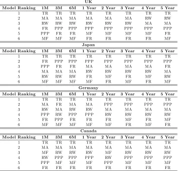
the study of Tables 1.1 and 1.2. According to the same tables, the technical rule appears to be, overall, the best model across horizons for the developed markets panel by beating the RW for almost all developed countries. The PPP model seems to perform better in the medium and long run. On the other hand, the MF model is found to forecast better at the 1-month horizon. The FR performs poorly across horizons except for the case of Japan. In general, the MSPEs become larger with longer horizons.

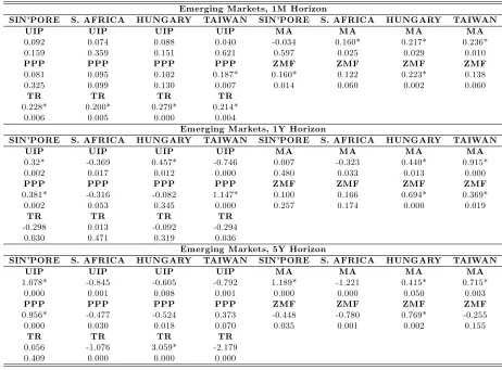
1.4.4. Emerging Markets Panel: Out-of-Sample Forecasting, Rolling Regressions Results

The rolling out-of-sample exercise does not display identical results for the emerg-ing markets panel. The overall picture suggests that it is more di¢ cult to fore-cast the emerging market currencies using either fundamental models or technical analysis. However, the model ranking with respect to forecasting performance is largely maintained. The FR model is consistently the worst performer in both panels with the MA model being the best across horizons. The TR model appears, again, to be very successful at the 1-month horizon. Finally, both the PPP and MF model performances appear notably weaker relative to the developed markets case. Again, the MSPEs get bigger with the forecasting horizon.

1.4.5. Forecast Combination: Rolling Regressions Results

(39)

over time and across horizons. The results for the 1-month horizon appear on Fig-ures 1.9 - 1.11. The picture is rather mixed; thep-values of the models’coe¢ cients display an evident time variation; in general one can see that di¤erent models are statistically signi…cant over time, providing further evidence to the hypothesis that market agents periodically revise the importance they assign to each model. As expected, as one moves to longer horizons the coe¢ cients tend to become more signi…cant.

Finally, the MSPE of the encompassing regression appears lower than the MSPE of the RW model, suggesting the existence of statistical gains from the combination of the models at 1-month horizon (see Table 1.3). When it comes to the robustness of this result, I refer to the inference procedure, developed by Clark and West (2006, 2007), for testing the null of equal predictive ability of two nested models. This methodology accounts for the fact that under the null the MSPE of the alternative model is projected to be larger than the one of the RW benchmark. This is due to the fact that the alternative model generates noise in the forecasting process by estimating a parameter vector that is not useful.

1.4.6. Is Technical Analysis a method of information processing?

(40)

and Papell (2009), contradicts the statement that exchange rates converge toward fundamental values only over longer horizons (Mark, 1995; Lothian and Taylor, 1996), as the TR model is found to display predictability even at 1-month ahead forecasts. Nevertheless, it is also true that there are often statistical gains from the combination of forecasts. It is, therefore, possible that these gains originate from chartism, since the TR speci…cation already incorporates a comprehensive set of fundamentals.

Figures 1.3-1.8 report the MSPE results. The comovement of the MA MSPE with the MSPE of other models is evident. The de…nition of the long-short MA pair itself embraces an error correction concept with the long MA element stand-ing for the "fundamental" value as determined by the market, consistent to the construction of other fundamental models. However, the inspection of the rolling regression plots of the MA model (Figure 1.1) rather complicates the picture. Al-though the coe¢ cients are consistently correctly signed and moving in opposite directions, statistical signi…cance is rarely gained. The most striking result is that this rarely happens when the long and short regression coe¢ cients cross, i.e. at the most informative points. In fact, signi…cance appears to be stronger when the coe¢ cient values diverge. In addition, as previously mentioned, the MA model does not fall in the MSPE rankings at longer forecasting horizons.

(41)

1.5. Economic Value

1.5.1. The Framework

This section details the framework employed for the economic evaluation of dif-ferent exchange rate (FX) strategies based on the models examined above. The exercise is conducted by evaluating the performance of a dynamically rebalanced portfolio following these strategies relative to a random walk benchmark. The eco-nomic analysis is again compiled out of sample. The in-sample period ranges from July 1989 until June 1998 and the out-of-sample period moves forward by succes-sively updating the parameter estimates of the forecasting equation on a monthly basis using a 10-year rolling window.

For the purposes of the exercise, I take the view of a US investor who builds a portfolio by allocating her wealth among eight assets that are identical in every aspect apart from the currency of denomination (GBP, JPY, EUR, CAD, SGD, ZAR, HUF and TWD). The main aim of this exercise is, thus, to establish whether there is economic value in predicting FX returns using each FX model separately, as well as their forecast combination. Throughout this analysis, I maintain the hypothesis that the risky assets constitute a zero-cost investment, and thus, the investor’s net balances gain interest at the domestic risk-free rate. This assumes that the return from each of the risky assets equals the domestic risk-free rate plus the currency return (it+ 1st+1). The return to a domestic risk-free investment is

approximated by the 1-month US Eurodeposit rate.

(42)

allocation1. Each month she takes two steps. First, she uses the respective model to forecast the cumulative long-short portfolio return. Second, conditional on the forecast, she dynamically reshu- es her portfolio following the long-short strategy described above.

In order to measure the economic value of each strategy, I rely on the com-putation of out-of-sample performance fees (as in Della Corte, Sarno and Sestieri, 2010), originally proposed by Goetzmann, Ingersoll, Spiegel and Welch (2007). This measure assumes neither a speci…c utility function nor a speci…c distribution of portfolio returns and it is de…ned as follows:

b 1

(1 ) tln 1 T

T

X

t=1

[(1 +rt)=(1 +rf t)]1

!

,

where thecstatistic is an estimate of the portfolio’s premium return after ad-justing for risk. T is the total number of observations, and tis the length of time between observations. These two variables annualize the measure. The portfolio’s un-annualized rate of return at timet isrt, and the risk-free rate isrf t:The coe¢

-cient of risk aversion should be selected to make holding the benchmark optimal for an uninformed manager.

Finally, when evaluating the pro…tability of the dynamic strategies, I don’t take into account the impact of transaction costs.

The out of sample predictions refer to the period between August 1999 and July 2009. The results indicate that there appears to be some economic value associated with the TR model, which outperforms all the other models, o¤ering an annualized performance fee of 105 basis points.

1_{This is a standard practice to market participants which is generally associated with hedge funds}

(43)

The results are displayed in Table 1.4, for a coe¢ cient of risk aversion = 3: Di¤erent risk aversion values do not change my results and hence I do not report them. The combined model (calculated over a shorter sample, between July 2002 and July 2009), the MA rule, the PPP model and the MF model, are all found to outperform the RW model but the economic gains appear to be small, except for the case of the combined model which provides an annualized performance fee of 89 basis points.

I …nally construct a combination strategy, allowing the investor to reassess her model choice on a monthly basis. Every period, she selects the best model in terms of statistical signi…cance (the one that displays the minimum average p-value across the eight currency pairs). The out-of-sample performance fees for this "p-value" combined model refer to the period between July 2002 and July 2009. The results show that the TR model is still ranked …rst, with the MA model being second beating the RW benchmark by 36 basis points. Nevertheless, it must be noted that due to data scarcity, the presented window is limited to few years and mainly covers the crisis period, something that could potentially distort the real picture.

1.6. Conclusion

Exchange rate forecasting has been a non-trivial endeavour throughout the lit-erature as it has been di¢ cult to empirically establish a link between fundamentals and exchange rate movements. Recent work in this …eld has employed Taylor rules to model exchange rate determination reporting promising results, as well as evi-dence of short term predictability. Furthermore, numerous studies have examined the pro…tability of chartist techniques suggesting the existence of signi…cant pro…ts in the foreign exchange market.

(44)

of fundamentals, a rich Taylor Rule speci…cation and a simple technical trading strategy, along with a model motivated by the literature on forecast combina-tions, I document three results. First, the Taylor rule model emerges as the best model, economically and statistically, at the 1-month horizon, displaying good per-formance across di¤erent countries. To my knowledge, this is the …rst time that the performance of this model has been assessed across di¤erent horizons, with a further emphasis put on the economic value of its predictions. The fact that the Taylor rule model appears to provide reliable short-term forecasts is an en-couraging result that appears to be robust both in the developed markets and the emerging markets under examination.

A second …nding of this study, is that the technical rule displays superior pre-dictive power over the random walk benchmark across horizons. The contribution of this result lies on the estimation frequency and the simplicity of the model em-ployed. Although the literature on the pro…tability of technical analysis suggests the existence of pro…ts, the majority of these studies target the implementation of these techniques at high frequency, or employs more sophisticated models. How-ever, my evidence suggests that there does not appear to be a horizon pattern in the performance of technical analysis. The …nding that traditional MA rules do not appear to be very pro…table in the 1990s is in line with the documented result that pro…ts from technical analysis are declining over time (Dooley and Shafer, 1983 and Sweeney, 1986 among others).

(45)

(46)

Appendix:In-Sample Estimation of the Models

In total, I estimate six models at eight horizons (1-month, 3-month, 6-month, 1-year, 2-year, 3-year, 4-year and 5-year ahead), for each of the eight countries. To illustrate whether the impact of technical analysis is stronger for emerging mar-ket currencies, I present the results for the emerging marmar-kets panel (Singapore Dollar, South African Rand, Hungarian Florint and Taiwanese Dollar) separately. The models are estimated by OLS rolling regressions using the Hodrick correction procedure (Hodrick, 1992) for the calculation of the standard errors of the long run regressions. As the data are sampled more …nely than the compound return interval, serial correlation of the error term is induced even if the null hypothesis of no predictability is true (Hansen and Hodrick, 1980). Consequently, the statistical inference in long horizons crucially relies on the choice of the standard errors. The Hodrick correction procedure corrects for heteroskedasticity and eliminates the moving average structure in the error terms, providing a reliable assessment of the statistical signi…cance of the estimated parameters. I, hence, evaluate the models’ predictive power by looking at the signi…cance of the estimated coe¢ cients. This constitutes a novel method of model assessment given the robustness of the proce-dure; essentially, by looking at the statistical signi…cance of the Combined model’s coe¢ cients, one is able to evaluate the models across horizons. Subsequently, the models are ranked in terms of the mean square prediction error (MSPE).

(47)

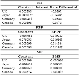
Tables 1A.1, 1A.2, 1A.3 and 1A.4 display the full sample estimated coe¢ cients for the developed markets panel for the 1-month horizon. The Fama regression is, as expected, consistent with carry trade activity, displaying a negative coe¢ cient which is statistically signi…cant for Japan. As far as the MA model is concerned, one can notice that the coe¢ cients are correctly signed though insigni…cant and moving in opposite directions. The same is true for the PPP model, while the coe¢ cients of the MF appear both inconclusive and insigni…cant. Finally, the real exchange rate coe¢ cient displays some consistency in the TR model but signi…-cance is still not gained at this horizon.

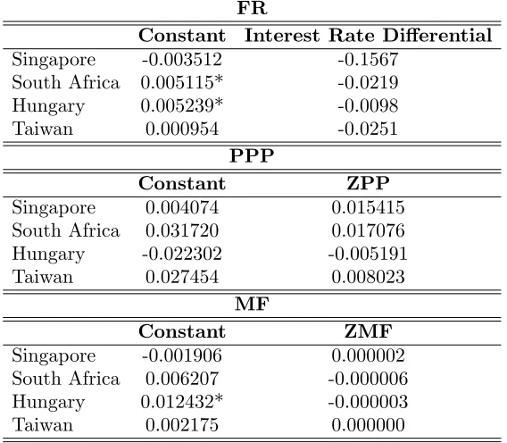
The combined model results are inconclusive, as di¤erent models perform best for di¤erent countries. However, an important issue that emerges at this stage is that one can extract statistical value from potentially all the models, at least for particular forecasting horizons. This …nding is more evident during the examina-tion of the rolling estimaexamina-tion results. Inspecexamina-tion of Tables 1A.5, 1A.6, 1A.7 and 1A.8 reveals similar results for the emerging market panel.

(48)

(49)

[image:49.612.189.455.266.519.2]

Appendix Tables

Table 1A.1. Full Sample Results for the Developed Markets Panel: Regression Coe¢ cients for the FR, PPP and MF Model

FR

Constant Interest Rate Di¤erential

UK 0.002753 -0.0991

Japan -0.008016* -0.1453*

Germany -0.002481 -0.0633

Canada 0.000598 -0.0473

PPP

Constant ZPPP

UK -0.007964 0.019022

Japan 0.076053 0.016861

Germany 0.005295 0.014344

Canada 0.002598 0.011987

MF

Constant ZMF

UK 0.001809 -0.000005

Japan -0.004664 0.000005

Germany -0.001870 0.000001

Canada 0.003574 -0.000012

(50)

Table 1A.2. Full Sample Results for the Developed Markets Panel: Regression Coe¢ cients for the MA Model

MA

Constant MA5 MA150

UK -0.017637* 0.039045 -0.07338

Japan 0.037552 0.00526 -0.01332

Germany 0.007464 0.025638 -0.03978

Canada 0.003297 0.054901 -0.06854

(51)

Table 1A.3. Full Sample Results for the Developed Markets Panel: Regression Coe¢ cients for the TR Model

Taylor Rule

Constant p p* y y* q i i*

UK -0.039802 -0.045681 0.051856 -0.003045* 0.002375 -0.025016 -0.000523 0.000685 Japan 0.391160 -0.092982 0.043369 0.000167 -0.002628 -0.036628* -0.001341 0.002896* Germany -0.129352 0.044612 -0.016111 -0.000895 0.000711 -0.020848 0.000547 0.001367 Canada 0.020294 0.006317 -0.010212 0.000027 0.001164 -0.010042 -0.000623 0.000393

(52)

Table 1A.4. Full Sample Results for the Developed Markets Panel: Regression Coe¢ cients for the Combined Model

Combined Model

Constant FR MA PPP MF TR

UK -0.000082 -1.658465* 0.264569 -0.002191 -0.473578 0.023336

Japan 0.484045 -0.145764 0.724338 0.151052 0.151052 -1.682664

Germany 0.331359 -0.001126 -0.777185* -0.259003 0.000147 0.697276*

Canada -1.196255 -0.964475* -0.195935 -0.461072 -0.402442 -0.174180

(53)

[image:53.612.181.465.151.399.2]

Table 1A.5. Full Sample Results for the Emerging Markets Panel: Regression Coe¢ cients for the FR, PPP and MF Model

FR

Constant Interest Rate Di¤erential

Singapore -0.003512 -0.1567

South Africa 0.005115* -0.0219

Hungary 0.005239* -0.0098

Taiwan 0.000954 -0.0251

PPP

Constant ZPP

Singapore 0.004074 0.015415

South Africa 0.031720 0.017076

Hungary -0.022302 -0.005191

Taiwan 0.027454 0.008023

MF

Constant ZMF

Singapore -0.001906 0.000002

South Africa 0.006207 -0.000006

Hungary 0.012432* -0.000003

Taiwan 0.002175 0.000000

(54)

Table 1A.6. Full Sample Results for the Emerging Markets Panel: Regression Coe¢ cients for the MA Model

MA

Constant MA5 MA150

Singapore 0.011016 -0.027794 0.002482

South Africa 0.015859 0.037096 -0.044406

Hungary 0.053845* 0.032864 -0.042705

Taiwan 0.052113 0.039274 -0.054316

(55)

Table 1A.7. Full Sample Results for the Emerging Markets Panel: Regression Coe¢ cients for the TR Model

TR

Constant p p* y y* q i i*

Singapore -0.224338 0.094582 -0.047495 -0.000056 -0.000187 -0.002285 -0.001896 0.001502 South Africa -0.073294 0.013788 0.012909 0.001661 -0.001679 -0.037257 0.000416 0.003226 Hungary 1.159206* 0.024430 -0.205808 -0.000191 -0.000972 -0.068495* 0.000061 0.003186 Taiwan -0.064798 0.015067 0.020099 0.000276 -0.000747 -0.028863 -0.000068 0.000631

(56)

Table 1A.8. Full Sample Results for the Emerging Markets Panel: Regression Coe¢ cients for the Combined Model

Combined Model

Constant FR MA PPP MF TR

Singapore -0.002562 0.749451 0.804480 -0.021708 -0.851484 2.9392091*

South Africa 2.123094* 0.80614138* 1.579366 -0.996874 1.2467491* 2.6705427*

Hungary -0.058931 -0.002622 0.325215 2.5918868* -0.004568 -1.045729

Taiwan 2.3316166* -2.490704 1.0625556* 0.387007 0.941339 1.0770411*

(57)

[image:57.612.148.499.151.488.2]

Table 1A.9. Full Sample Results for the Developed Markets Panel: Model Ranking across Horizons

UK

Model Ranking 1M 3M 6M 1 Year 2 Year 3 Year 4 Year 5 Year

1 TR TR TR TR TR TR TR TR 2 MA MA MA MA MA MA RW RW 3 RW RW RW RW RW RW MA MA 4 FR PPP PPP PPP PPP PPP PPP PPP 5 PPP FR FR MF MF MF MF FR 6 MF MF MF FR FR FR FR MF

Japan

1 TR TR TR TR TR TR TR TR 2 FR PPP PPP PPP PPP PPP PPP PPP 3 PPP FR FR MA MA MA MA FR 4 MA MA MA RW RW RW RW MA 5 RW RW RW FR MF FR MF RW 6 MF MF MF MF FR MF FR MF

Germany

1 TR TR TR TR TR TR TR TR 2 MA FR MA MA PPP PPP PPP PPP 3 RW MA RW RW MA MA MA MA 4 PPP RW PPP PPP RW RW RW RW 5 FR PPP FR FR FR MF FR MF 6 MF MF MF MF MF FR MF FR

Canada

1 TR TR TR TR TR TR TR TR 2 MA MA MA MA MA MA MA MA 3 MF RW RW RW MF RW RW RW 4 RW PPP PPP PPP RW PPP PPP PPP 5 PPP MF MF MF PPP MF MF MF 6 FR FR FR FR FR FR FR FR

(58)

[image:58.612.148.499.150.489.2]

Table 1A.10. Full Sample Results for the Emerging Markets Panel: Model Ranking across Horizons

Singapore

1 TR TR TR TR TR TR TR TR 2 FR FR MA MA MA MA MA MA 3 RW RW RW RW RW RW RW RW 4 MA MA PPP FR PPP PPP PPP PPP 5 PPP PPP FR PPP FR FR FR FR 6 MF MF MF MF MF MF MF MF

South Africa

1 TR TR TR TR TR TR TR TR 2 MA PPP PPP PPP PPP PPP PPP PPP 3 PPP MA MA MA MA RW RW RW 4 RW RW RW RW RW MA MA MA 5 FR FR FR FR FR MF MF MF 6 MF MF MF MF MF FR FR FR

Hungary

1 TR TR TR TR TR TR TR TR 2 MF MA MA MA MF MA MA MA 3 MA MF RW MF MA MF RW RW 4 RW RW MF RW RW RW MF MF 5 PPP PPP PPP FR FR FR FR FR 6 FR FR FR PPP PPP PPP PPP PPP

Taiwan

1 TR TR TR TR TR TR TR TR 2 MA MA MA MA PPP PPP PPP PPP 3 RW RW RW RW MA RW RW MA 4 PPP PPP PPP PPP RW MA MA RW 5 MF MF MF FR FR FR FR FR 6 FR FR FR MF MF MF MF MF

(59)

[image:59.612.114.532.192.563.2]

Tables

Table 1.1. Out-of-Sample Forecasting Ability: Developed Markets

Developed Markets, 1M Horizon

UK JAPAN GERMANY CANADA UK JAPAN GERMANY CANADA

UIP UIP UIP UIP MA MA MA MA

0.050 0.122* 0.066 0.094 0.139* 0.111* 0.111* 0.121

0.368 0.007 0.177 0.061 0.003 0.014 0.014 0.059

PPP PPP PPP PPP ZMF ZMF ZMF ZMF

0.121* 0.102 0.077 0.119* 0.085 0.105* 0.100* 0.140*

0.008 0.550 0.056 0.008 0.100 0.015 0.024 0.002

TR TR TR TR

0.180* 0.203* 0.262* 0.196*

0.000 0.000 0.000 0.001

Developed Markets, 1Y Horizon

0.089 -0.019 -0.187 0.049 0.307* 0.529* 0.495* 0.268*

0.155 0.425 0.025 0.294 0.001 0.000 0.000 0.010

0.170* 0.521* 0.434* 0.191 0.072 -0.016 0.057 -0.115

0.037 0.000 0.000 0.056 0.250 0.447 0.302 0.138

TR TR TR TR

0.133 0.035 -0.210 0.178

0.084 0.391 0.025 0.052

Developed Markets, 5Y Horizon

0.246 0.589* -0.578 0.635* 0.470* 0.594* 0.886* 0.491*

0.051 0.000 0.000 0.000 0.001 0.000 0.000 0.001

0.478* 0.382* 0.898* 0.525* 0.013 0.353* 0.198 -0.281

0.001 0.006 0.000 0.000 0.467 0.010 0.102 0.038

TR TR TR TR

0.291* 0.068 0.286* 0.297*

0.022 0.322 0.034 0.018

(60)

[image:60.612.112.574.154.495.2]

Table 1.2. Out-of-Sample Forecasting Ability: Emerging Markets

Emerging Markets, 1M Horizon

SIN’PORE S. AFRICA HUNGARY TAIWAN SIN’PORE S. AFRICA HUNGARY TAIWAN UIP UIP UIP UIP MA MA MA MA

0.092 0.074 0.088 0.040 -0.034 0.160* 0.217* 0.236* 0.159 0.359 0.151 0.621 0.597 0.025 0.029 0.010

0.081 0.095 0.102 0.187* 0.160* 0.122 0.223* 0.138 0.325 0.099 0.130 0.007 0.014 0.060 0.002 0.060

TR TR TR TR

0.228* 0.200* 0.279* 0.214* 0.006 0.005 0.000 0.004

Emerging Markets, 1Y Horizon

0.32* -0.369 0.457* -0.746 0.007 -0.323 0.440* 0.915* 0.002 0.017 0.012 0.000 0.480 0.033 0.013 0.000

0.381* -0.316 -0.082 1.147* 0.100 0.166 0.694* 0.369* 0.002 0.053 0.345 0.000 0.257 0.174 0.000 0.019

TR TR TR TR

-0.298 0.013 -0.092 -0.294 0.030 0.471 0.319 0.036

Emerging Markets, 5Y Horizon

1.078* -0.845 -0.605 -0.792 1.189* -1.221 0.415* 0.715* 0.000 0.001 0.008 0.001 0.000 0.000 0.050 0.003

0.956* -0.477 -0.524 0.373 -0.448 -0.780 0.769* -0.255 0.000 0.030 0.018 0.070 0.035 0.001 0.002 0.155

TR TR TR TR

0.056 -1.076 3.059* -2.179 0.409 0.000 0.000 0.000

(61)

Table 1.3. Out-of-Sample Forecasting Ability: Combined Model, Developed and Emerging Markets

Developed Markets, 1M Horizon Emerging Markets, 1M Horizon

UK JAPAN GERMANY CANADA SIN’PORE S. AFRICA HUNGARY TAIWAN Combined Combined Combined Combined Combined Combined Combined Combined

0.264* 0.406* 0.480* 0.331* 0.557* 0.591* 0.508* 0.543* 0.000 0.000 0.000 0.000 0.000 0.000 0.000 0.000

Developed Markets, 1Y Horizon Emerging Markets, 1Y Horizon

-0.116 0.337* -0.025 0.116 -0.262 0.261 -0.059 0.168 0.165 0.002 0.415 0.180 0.089 0.096 0.381 0.155

Developed Markets, 5Y Horizon Emerging Markets, 5Y Horizon

0.390* 0.154* 0.225* -0.010 -0.555 -0.022 -0.136 -0.250 0.000 0.035 0.004 0.453 0.004 0.454 0.201 0.081

(62)

Table 1.4. Calculation of Performance Fees

Performance Fees, Aug 1999-July 2009

FR MA PPP MF TR

-8 37 24 20 105

Performance Fees, Jul 2002-July 2009

FR MA PPP MF Combined TR

-10 36 13 20 89 105

Performance Fees, Jul 2002-July 2009

FR MA PPP MF Combined, Min p-val TR

-10 36 13 20 18 105

(63)

Figures -0.4 -0.2 0.0 0.2 0.4 0.6 0.8 1.0 1.2

86 88 90 92 94 96 98 00 02 04 06 08 UK_M1 UK_M2 UK_PVAL_M1 UK_PVAL_M2 GBP_USD -0.2 0.0 0.2 0.4 0.6 0.8 1.0 1.2

86 88 90 92 94 96 98 00 02 04 06 08 JAPAN_M1 JAPAN_M2

JAPAN_PVAL_M 1 JAPAN_PVAL_M 2 JPY_USD -0.2 0.0 0.2 0.4 0.6 0.8 1.0 1.2

86 88 90 92 94 96 98 00 02 04 06 08 GERMANY_M1 GERMANY_M2 GERMANY_PVAL_M1 GERMANY_PVAL_M2 DEM_USD -0.2 0.0 0.2 0.4 0.6 0.8 1.0 1.2

86 88 90 92 94 96 98 00 02 04 06 08 CANADA_M1 CANADA_M2

[image:63.612.137.553.425.631.2]

CANADA_PVAL_M1 CANADA_PVAL_M2 CAD_USD