Continuous Chain Ladder: Reformulating and generalizing a classical insurance problem

      

City, University of London Institutional Repository

Citation

:

Martinez-Miranda, M. D., Nielsen, J. P., Sperlich, S. and Verrall, R. J. (2013). Continuous Chain Ladder: Reformulating and generalizing a classical insurance problem. Expert Systems with Applications, 40(14), pp. 5588-5603. doi: 10.1016/j.eswa.2013.04.006

This is the unspecified version of the paper.

This version of the publication may differ from the final published

version.

Permanent repository link:

http://openaccess.city.ac.uk/3757/

Link to published version

:

http://dx.doi.org/10.1016/j.eswa.2013.04.006

Copyright and reuse:

City Research Online aims to make research

outputs of City, University of London available to a wider audience.

Copyright and Moral Rights remain with the author(s) and/or copyright

holders. URLs from City Research Online may be freely distributed and

linked to.

City Research Online: http://openaccess.city.ac.uk/ [email protected]

Continuous Chain Ladder

Mar´ıa Dolores Mart´ınez Miranda

University of Granada, Spain [email protected]

Jens Perch Nielsen

Cass Business School, City University, London, U.K. [email protected], [email protected]

Stefan Sperlich

Universit`e de Gen`eve, D´epartement des sciences ´economiques Bd du Pont d’Arve 40, CH - 1211 Gen´eve 4

[email protected]

Richard Verrall

Cass Business School, City University, London, U.K. [email protected]

February 11, 2013

Abstract

To be written

Keywords: Chain Ladder; Claims Reserves; Reserve Risk; Multiplica-tive bias correction; Density estimation, Crossvalidation; smoothing; kernel.

1

Introduction

A key feature of the vast majority of claims reserving methids used in practice, including the CLM, is that they assume that the data have been aggregated. This aggregation is often done by year, but it could also be done by quarter or month. Whatever time period is used, the key point to note is that this aggregation implies some pre-smoothing of the data. Claims reserving methods which use continuous models (parametric or non-parametric) have been suggested in the literature but they almost invariably involved the use of aggregated data which has therefore been reduced to discrete time data. The approach of this paper is different in that it does not assume that the data have been aggregated: it uses data recorded in continuous time. As this is a new approach, we present methods which are close to the CLM, but we keep them as straightforward as possible. It would be possible to add sophistication to these, but this would detract from the simplicity of the presentation and we leave this for future work. Because the appraoch uses data recorded in continuous time and is based on the philosophy underlying the CLM, it can be viewed as a continuous version of the CLM. For this reason, we have named it ” Continuous Chain Ladder”.

Methods based on data recorded over a continuous time scale have previ-ously been suggested in the actuarial literature (e.g. Norberg, 1986), but the papers only rarely addressed the implementation of these methods. In the practical context the results have generally been somewhat disappointing. We believe that this somewhat disappointing outcome for continuous reserv-ing so far is that the methods have been too distant from well-known methods such as the CLM to appeal to actuaries. This paper therefore aims to show how reserving using data recorded in continuous time can be viewed as a natural transition from CLM to sophisticated modern statistical methods.

nonparamet-ric smooth backfitting of Yu, Park and Mammen (2008). This is related to the approach taken in this paper, because the multiplicative model can be regarded as a generalized additive model.

The paper is structured as follows...

2

The classical model for aggregated data

One of the most popular method used in reserving is the classical chain ladder method (CLM) which uses simple aggregated triangular arrays of data. Several stochastic models for CLM have been formulated which model directly the aggregated data (see for example Verrall and England 2002, or W¨uthrich and Merz, 2008). This paper considers a new and modern approach based on smoothing methods which will provide a different perspective on claims reserving, which gives more insights into classical reserving methods such as the CLM. This section describes briefly the classical formulation which will be a benchmark throughout the paper.

In classical reserving methods it is assumed that the available information is a run-off triangle with dimensionm, i.e. a triangle withmrows. Thus, the information is provided in an aggregated way where, in theory, any aggrega-tion periods could be considered, such as quarters, years etc. Depending on the data being considered, each cell in the triangle could contain the number of reported or paid claims (counts data) or aggregated payments (reported or paid). Traditional methods such as the CLM are often applied to all of these types of triangles, with different distributional assumptions used as ap-propriate. For example, a Poisson model would be suitable for counts and an over-dispersed Poisson for aggregated payments. This paper considers only counts in order to make the density approach as clear as possible. The extension to payments data will be considered in future work.

We assume, without loss of generality, that the data are available as a triangle, and denote the set indexing the periods for which the data are available by Im = {(i, j) : i = 1, . . . , m, j = 1, . . . , m; i+j − 1 ≤ m}.

Here i denotes the origin period and j the delay period (i.e. j −1 periods delay from i). The aggregated incurred counts triangle can then be written by ℵm = {Nij : (i, j) ∈ Im}, where Nij is the total number of claims of

insurance incurred in period i, which are reported in period i+j −1 i.e. with j−1 periods delay from year i. An example of such aggregated data is shown in the top graph in Figure 1. This data set corresponds to numbers of reported claims (incurred counts) observed for claims that were incurred in the m= 19 past years.

methods and it is possible to predict the outstanding claims and construct a reserve starting from aggregated data. In order to do this, the methods produce projections in the lower and unexperienced triangle Jm = {(i, j) :

i= 2, . . . , m, j = 1, . . . , m; i+j−1> m}. The traditional CLM projections can be derived from maximum likelihood estimation under a Poisson model for the aggregated data (see Kuang, Nielsen and Nielsen, 2009). Note that such a model is often quite a reasonable model for counts data. Thus, it is assumed that the cells in the triangle are independently Poisson distributed with cross-classified mean, which is specified by the following multiplicative parametrization:

E[Nij] =αiβj, (i, j)∈ Im. (1)

By solving the well-known identification problem for this kind of method (see Kuang, Nielsen and Nielsen, 2009), standard tools from generalized linear models provide estimates for the parameters αi and βj, for i, j = 1, . . . , m.

From these estimates the predicted outstanding claims for each underwriting period are obtained by summing the predicted values for the claims in the lower triangle by row. Also, outstanding claims for future calendar period can be predicted by summing the diagonals in the lower triangle. Both calculations are the common output required from reserving methods. An illustration of the classical chain ladder method on real insurance data is given in Section 5. The next section introduces the continuous approach which underlies the new method proposed in this paper.

2.1

A regression view of the density estimation

prob-lem

As indicated above, the aim of this paper is firstly to reformulate the re-serving problem in terms of a multivariate density estimation problem and then to develop kernel methods to estimate nonparametrically this density. The classical CLM provides one approach to this non-parametric density es-timation problem as is explained in this subsection. This new perspective on further understanding classical reserving methods such as the CLM can provide greater understanding and may also be the key to makel progress in developing modern and powerful methods.

exposi-tion more straightforward. Let X1, . . . , Xn be a random i.i.d. sample from a

population X with continuous density f. Let a1 <· · · < am denote equally

spaced grid points definingm−1 contiguous intervals or binsBj = (aj, aj+1],

for j = 1, . . . , m−1. The extreme points a1 and am are typically chosen in

such a way that the support of f is contained in (a1, am]. Let Λm denote the

bin size (Λm =a2−a1). Also for eachj = 1, . . . , m, letxj denote the bin

cen-ter (xj = (aj+1+aj)/2), and Nj the bin count defined as the number of data

falling in the interval Bj. It is clear that Nj follows a binomial distribution

with size parameter n and success probability pj = R

Bjf(x)dx. Therefore

whenm→ ∞or equivalently Λm →0 we have the following approximations:

E

Nj

nΛm

≈f(xj)

and

V

Nj

nΛm

≈ f(xj)

nΛm

,

forj = 1, . . . , m. Thus the density problem is equivalent to a heteroscedastic regression problem based on the data, {(xj, Nj/Λmn), j = 1, . . . , m}, which

are approximately independent. Equivalently the regression model can be written for the bin counts Nj as

Nj =r(xj) +εj, (2)

with r(·) = nΛmf(·) being the regression function. From a regression

esti-mate _br(·) the target density can be estimated as fb(·) =r(·)nΛ_m.

Now if we move to the two-dimensional scenario it can clearly be seen that the classical chain ladder method approaches the density problem through the regression formulation in equation (2). Specifically, the CLM estimates a two-dimensional densityf supported in the triangleIm and using a multiplicative

structure. The bins are constructed as squares of the form Bij = (ai, ai+1]×

(bj, bj+1], for i, j ∈ Im, with bin length Λm = a2 − a1 = b2 −b1 being

constant. Thus, from the bin counts Nij (the number of data falling in Bij)

the regression problem can be formulated as

Nij =r(zij) +εij, (3)

based on the data {(zij, Nij, i, j ∈ Im}. The two-dimensional covariate

zij = (xi, yj), is defined such thatxi andxj are the midpoints of the intervals

(a1,i, a1,i+1] and (a2,j, a2,j+1], respectively, for i, j ∈ Im. The regression

func-tion is then related with the density byr(·,·) = nΛmf(·,·). By assuming that

the problem can be solved using classical generalized linear models (GLM) with the logarithm as the link function and some specified error distribu-tion (see for example England and Verrall, 2002, for a descripdistribu-tion of this approach). The classical Poisson (for claim counts) as defined by equation (1) relies on the Poisson approximation of the binomial distribution. Clearly each bin count, Nij, follow a binomial distribution with parameters n and

pij, where n is the total ultimate number of claims for each accident year

and pij = R

Bijf(z)dz. It is well known that the binomial distribution can

be approximated by a Poisson distribution: Nij ,→P(npij), which justifies a

GLM model with log link function and Poisson error distribution. Note that the largern and the smallerpij the better is the approximation and therefore

the expected performance of the classical CLM.

The above description shows how CLM focuses on the regression approach when considering the estimation of a density and thus it can only work on binned data. The following section describes methods which aim to estimate the underlying density and which are therefore more suited to the consider-ation of individual data using continuous time.

3

The continuous density approach

3.1

From the histogram to kernel smoothing

Kernel methods for density estimation arise in an intuitive and natural way from the naive histogram estimator. The application of these kernel meth-ods in reserving relies on the recognition that the classical CLM consists of the construction of a structured histogram on a triangle. A histogram is the simplest nonparametric approach to estimate a density function. The his-togram separates the data into distinct non-overlapping bins, and constructs bars (hypercubes) with heights defined as the proportion (or the number) of observations falling into each bin. This proportion gives an estimate of the probability density function at the mid point of the bin (see subsection 2.1). As in Section 2.1 we start from the simpler univariate scenario and extend this afterwards to the two-dimensional situation. Consider again a random sample, X1, . . . , Xn, from a population X with a continuous

den-sity f. Consider m−1 contiguous intervals Bj = (aj, aj+1] or bins with bin

length Λm, which divide the support of f, and let xj be the midpoints, for

j = 1, . . . , m−1. The height of the bar of the histogram with baseBj provides

an estimate of the probability density function at the midpoint,xj. Thus, an

estimator of the density f at any pointx0 in the support off can be derived

from the limit concept of ratio between probability mass in a neighborhood of a point and the size of the neighborhood. Using proper mathematics it is an application of the mean value theorem of integral calculus, which implies that

lim

Λm→0

P(X ∈Bj)

Λk

=f(x) if x∈Bj (j = 1, . . . , m−1).

From this expression the histogram estimator at any point x0 in the support

is defined by

b

fhist(x0) =

n−1Pn

i=1I{Xi ∈Bj}

Λm

if x0 ∈Bj (j = 1, . . . , m).

Note that the histogram is not a continuous function, but has jumps at the grid points and has zero derivative everywhere else. This gives estimates which are not only aesthetically undesirable, but, more seriously, could pro-vide to an untrained observer with a misleading impression. In fact, the shape of the histogram can potentially be influenced by where the bin cen-tres are placed. From the above formulation, these are defined by the choice of the width Λm and the location of the first point a1. Partly to overcome

Moving now to the two-dimensional scenario, assume that Z1, . . . , Zn is

an i.i.d. random sample from a population Z = (X, Y), having bivariate continuous density f. Consider a split of the support of f into squares of the form Bij = (a1,i, a1,i+1]×(a1,j, a2,j+1], with constant length of the sides

Λm =a1,2−a1,1 =a2,2−a2,1. Following analogous arguments to those used

in the univariate case, the simple histogram estimator can be defined at any point z0 = (x0, y0) in the support of f by

b

fhist(z0) =ν(z0)/nΛ2m,

whereν(z0) is the number of sample data falling in the square which contains

z0. From this formulation the typical kernel density estimator can be seen as

a moving histogram which defines the bins centered at each point where the density is estimated. In this case the bins can overlap and the data falling in the bin are given different weights according to their proximity to the esti-mation point. Thus, the kernel estimator overcomes the problem of the naive estimator concerning the location of the bins but also it provides a smooth estimate for the target continuous density. The simplest kernel density esti-mator is the multivariate extension of the Parzen-Rosenblatt estiesti-mator. For any estimation point the support, z0 = (x0, y0) this is defined as

b

fh(z0) = |h|−1 n X

i=1

Kh(z0−Zi), (4)

where Kh(·) is a two-dimensional kernel and h = (h1, h2)t ∈ IR+2 is a

band-width parameter with|h|=h1h2. Here we use a simple multiplicative kernel

given byKh(u, v) = Kh1(u)Kh2(v) withKh1(u) = h

−1

1 K(u/h1) andK being a

unidimensional symmetric probability density function. This multiplicative structure is the more convenient for our purposes in the paper, but other general kernels such as spheric kernels could also be considered, and also more general bandwidth parameter such as matrices (see for example Wand and Jones, 1995, pp.103).

multiplicative structure and use the marginal integration method by Linton and Nielsen (1995) to provide a multiplicative local linear estimator for the density. This provides the required predictions in the forecast set (the lower triangle in the square).

3.2

The unstructured local linear estimator in the

ob-servation triangle

Nielsen (1999) extended the principle of local linear estimation by Lejeune and Sarda (1992) and Jones (1993) to nonparametric multivariate density estimation with arbitrary boundary regions. Let f denote a two-dimensional density having support in the triangle I = {z = (x, y)t|0 ≤ x, y ≤ T, x+

y ≤ T} with any T > 0. Here for simplicity we assume the origin period is equal to zero. Nielsen’s local linear estimator is defined at each point

z0 = (x0, y0)t ∈ I as the solution Θb0 of the following minimization problem:

b

Θ0 b

Θ1 !

= arg min

lim

b→0 Z

I

h

e

fb(z)−Θb₀−Θbt₁(z₀−z) i2

Kh(z−z0)dz

, (5)

where feb(z) = n−1(b1b2)−1Pn_i=1Kb(z−z0) is the standard kernel estimator

in (4) at the point z with bandwidth parameter b = (b1, b2)t ∈ IR2+ and

two-dimensional kernel K. As above in section 2.1 a multiplicative kernel,

K(x, y) = K(x)K(y) is used, with K being a unidimensional symmetric kernel function.

Note that this estimator is only defined in the observation triangle and therefore is not suitable for forecasting purposes. Recall that the forecast horizon is giving by J ={z = (x, y)t_{|0≤ x, y ≤ T, x+y > T}. In the next}

section we assume a multiplicative structure for the density and provide an estimator which can be used to provide forecasts in the lower triangle J.

3.3

The structured local linear density estimator

Now we assume that the target density in the whole square S = {z = (x, y)t_{|0 ≤ x, y ≤ T} is multiplicative i.e. f(x, y) = f}

1(x)f2(y). The

marginal integration method introduced by Linton and Nielsen (1995) can be extended to the density estimation problem in 3.2 through the following two-step method:

Step 1. From the available data estimate the two-dimensional density in the observation set I by an estimator fb_hI(x, y), such as the local

Step 2. Assume that the target density is multiplicative, f(x, y) =

f1(x)f2(y) and estimate f1 and f2 through the following minimisation:

minf1,f2

Z

I

b

f_hI(x, y)−f1(x)f2(y) 2

dxdy. (6)

The minimization at Step 2 can be performed using an iterative algorithm such as the following:

1. Consider an initial estimator of the componentf1 denoted byfb (0) 1 . Let b

f(0) denote the unstructured estimator for the density in I defined in Step 1 above.

2. Using fb (0)

1 , f(x, y)≈fb (0)

1 (x)f2(y) so that Z

Iy

f(x, y)dx≈f2(y) Z

Iy b

f₁(0)(x)dx

with Iy ={x|(x, y)∈ I}. Estimate the density f2 by

b

f₂(1)(y) =

R

Iyfb

(0)_{(x, y)dx} R

Iyfb (0) 1 (x)dx

.

3. Using fb (1)

2 , calculate the updated estimator for f1 by

b

f₁(1)(x) =

R

Ixfb

(0)_{(x, y)dy} R

Ixfb (1) 2 (y)dy

.

4. Repeat steps 2-3 until the desired convergence criterion is achieved.

This provides estimates for any point in the square S ={z = (x, y)t_|0≤

3.4

A multiplicative bias correction

In this section, we consider a second improved kernel estimator using bias reduction techniques. It is well-known that kernel methods such as those proposed above provide biased estimates. In the context of this paper, bias should be corrected since it could lead to incorrect reserves with serious consequences for the solvency of non-life insurers. Note that the variability is not so relevant because the insurer is usually interested in aggregated values of the estimates such as the total reserves for the future calendar years or even the overall total in the range of years under consideration.

There are several alternative bias reduction methods to correct the kernel estimates at points of large curvature. Here we consider the multiplicative bias correction (MBC) method proposed by Jones, Linton and Nielsen (1995) for univariate density estimation. The estimator is again introduced in two steps. Firstly a multiplicative bias corrected estimator for the density in the observation triangle is defined, which is an unstructured MBC estima-tor. Secondly, the marginal integration method is applied to provide the structured MBC density estimator.

Consider the unstructured local linear estimator defined in subsection 3.2. Denote this estimator by fb_LL,hI and recall that it is supported inI. The

unstructured MBC estimator is defined (having the same support) from the following expression:

b

f_{M BC,h}I (z) =fb_LL,hI (z) b

g_LL,hI (z) (7)

where _bg_LL,hI is the local linear estimator of the ratio f(z)/fb_LL,hI (z) obtained

by minimising the expression below in Ψ0.

minΨ0,Ψ1

lim

w→0

Z

I

e

g(z;w)−Ψ0−Ψt1(z0−z) 2

b

f_LL,hI (z)

−1

Kh(z−z0)dz

(8) Now from the estimator defined in (7) and using a similar method to that described in subsection 3.3 the MBC estimators of the univariate densities

f1 and f2 are obtained, together with the structured MBC estimator as their

product.

3.5

Choice of degree of smoothing

estimate the theoretically optimal bandwidths are unfeasible in practice and therefore it is necessary to provide a reasonable data-driven bandwidth es-timate. The problem of bandwidth selection also arises also when other estimators such as smoothing splines are used. In this case the smoothing parameter defines the appropriate weightings of fit andd smmothness. Sec-tion 4 describes some of the approaches that have been previously considered in the reserving literature.

For the kernel density estimators defined above, the bandwidth is a two-dimensional parameter h = (h1, h2) which controls the degree of smoothing

in each direction. Specificallyh1 andh2 move between 0 and infinity, thereby

corresponding to extreme cases of undersmoothing and oversmoothing, re-spectively. h1 defines the degree of smoothing in the underwriting direction

and h2 in the development direction.

There are several possible methods suggested in the literature to choose the bandwidth for a two-dimensional density. One of the simplest and most commonly used is the crossvalidation method (see for example Wand and Jones 1995). The crossvalidation method is an in-sample technique which aims to estimate the optimal bandwidth for the estimator using the sample data. In this paper, two candidates are suggested to estimate the density from a sample in the reserving triangle using a multiplicative structure. These are the local linear estimator and a multiplicative bias-corrected version. We propose here simply to use crossvalidation to find good unstructured density estimators in the observed triangle, and from such estimators to calculate the corresponding structured densities following the method described in Section 3.3.

For either of the unstructured density estimators defined in the triangleI, the LL estimator (fb_LL,hI ) or the MBC estimator (fb_{M BC,h}I ), the cross-validation

score is defined by

CV(h) =

Z

I

b

f_hI(z)2dz−2

n X

i=1 Z

I

b

f_hI,[−i](z)dFe_n(z), (9)

withfb

I,[−i]

h being the leave-one-out version of the estimatorfb_hI, andFe_n being

4

Related nonparametric methods in

reserv-ing

The reserving literature contains other suggestions for smoothing methods, and these can be related to the kernel density methods proposed in this paper. The aim of this section is also to demonstrate the novelty of the approach in this paper.

An early paper where the notion of smoothing is applied to the reserving problem is Verrall (1996) which was followed by England and Verrall (2001). The latter paper formalizes a traditional approach in actuarial practice which consists of smoothing the development factors in the deterministic chain lad-der approach. England and Verrall (2002) contains a description of this and further develops it in the framework of the generalized linear models (GLM). Chain ladder models are parametric models where the number of parameters increases in a linear way with the dimension of the run-off triangle. From a triangle of dimension m and assuming the Poisson model for the entries in the triangle with multiplicative structure such as (1), the log-likelihood can be written as

L(αi, βj;ℵm) =

X X

(i,j)∈Im

{−αiβj +αiβjlog(Nij)}, (10)

(omitting a constant term). Verrall (1991) and Kuang, Nielsen and Nielsen (2009) proved that the maximum likelihood estimators, {α_bi, βj,1 ≤ i, j ≤

m}, provide the chain ladder estimates by Nb_ij = α_biβb_j, for each i, j =

1, . . . , m. The intuition in this paper indicates that low levels of aggregations in the triangle would lead to serious problems in the likelihood behavior.

Apart from the well-known problem of identification of the parameters, which was solved by Kuang, Nielsen and Nielsen (2008), maximum likelihood methods tend to break down when the dimension goes to infinity. Grenan-der’s method of sieves was suggested (Greman and Hwang 1982) as a method for modifying classical estimators so as to make them appropriate for such nonparametric problems. When the dimension of the parameter space goes to infinity, it is suggested that the optimization is attempted within a subset of the parameter space, with this subset then being alowed to increase with the sample size. The sequence of subsets from which the estimator is drawn is called a “sieve” and therefore the resulting estimation method is called the “method of sieves”. Also the growth rate is controlled by the sieve size which, in practice, has to be chosen .

max-imum likelihood estimator based on an i.i.d. sample, X1, . . . , Xn, is defined

as the maximizer ofL(f;X1, . . . , Xn) = Πni=f(Xi). If nothing is known about

the target density the maximum cannot be achieved. This problem could be solved by restricting the set of candidates where the optimization is carried out. A sieve can be defined for this problem as the following sequence

sf,m ={f :f is a p.d.f. constant onBj j = 1, . . . , m}

with Bj being m contiguous intervals or bins dividing the support of f with

bin size equal to Λm. Then the method of sieves consists of maximizing

the likelihood L in the subspace sf,m, allowing m to grow with the

sam-ple size n. The solution, which is thus a sieve estimator, is the well-known histogram estimator which was described in Section 2.1. Other examples in density estimation include penalized maximum likelihood estimators. A kernel smoother such as the simple Parzen-Rosemblat-type estimator, de-scribed in Section 3.1, is close to the sieves method but differs in the fact that it is not a maximum likelihood estimator for the density (see Greman and Hwang, 1982, for more details). Thus, the kernel approach in this paper moves away from the classical method of sieves to the modern and power-ful kernel smoothing theory where good estimators such as the local linear and the multiplicative bias corrected estimators can attain good theoretical properties with excellent practical performance.

The flexible method proposed by England and Verrall (2001) is quite close to the above method of sieves. In this case the relation comes from an application to regression, also described by Greman and Hwang (1982), where a particular choice of sieve leads to the well-known smoothing splines estimator for the univariate regression function. Again, it is known that the maximum likelihood estimator is not consistent when a nonparametric (of infinite dimensional parametric) regression function is assumed. A sieve for this problem can be defined as the set of absolutely continuous functions r

satisfying R |r0(x)|2dx≤m, and the sieves estimator would be a first degree polynomial smoothing spline (see for example Fan and Gijbels 1996 for a description of smoothing regression splines). England and Verrall (2001) ex-ploits the regression formulation of the reserving problem to apply smoothing ideas. The approach of this paper becomes more complex than in Greman and Hwang (1982), but the aim is still to provide estimators having the max-imum likelihood properties in a nonparametric framework. The aproach of England and Verrall (2001) is described here, in order to make the connection with the classical method of sieves clear, and also to show thel connection with the kernel methods suggested in this paper.

could be Poisson (as considered here) but also gamma, inverse gamma etc. Such a variety of distributions allows the GLMs to be used for bothe claim claims and claim amounts triangles, with the Poisson model being suitable for the counts triangle, and an overdispersion property often used for the triangle of paid claims. Denoting by Cij the entries in any of these triangles

the above distribution can be characterized by the following assumption for the variance:

V(Cij) = φmρij,

with E[Cij] = mij. Values of ρ = 1,2 and 3 give the Poisson, gamma and

inverse gamma, respectively. We focus on one of the GLM modesls for the mean for the data in a triangle, given by:

log (mij) =c+ai+bj. (11)

Here the use of the logarithmic transform makes the model linear but it also imposes some positivity constraints on the data in the triangle. This para-metric model is usually fitted in practice using standard GLM tools. Note that if the dimension of the triangle is allowed to grow (and hence also the number of parameters in (11) increases), it would again give rise to a non-parametric maximum likelihood problem. Here the method of sieves would suggest defining a sieve candidate which could lead to consistent solutions. This was not the motivation of England and Verrall (2001), where a new and flexible model is described which could generalize simpler models such as that specified in equation (11) or others such as the so called Hoerl curve given by

log (mij) = c+ai+bilog(j) +γij. (12)

In this case, generalized additive models (GAMs) can be used of the following form:

log (mij) = sθi(i) +sθj(log(j)) +sθj(j). (13)

In this, sθi and sθj are smoothers for the underwriting period i and the

development period j, with smoothing parameters θi, and θj, respectively.

The extremes values for the smoothing parameters i.e. zero and infinity, would lead to either the classical chain ladder model in (11) or the Hoerl curve in (12), respectively. Smoothing splines smoothers were considered for

sθi and sθj, thereby considering the underwriting and development periods

as continuous variables.

H¨ossjer, Ohlsson and Verrall (2011), where smoothing is introduced moti-vated by what is often done inl practice in reserving by an actuary: the smoothing of the development parameters using just ad hoc truncations of the estimated values from the chain ladder method.

All these smoothing approaches in reserving have a relationship with the general method of sieves, even though the nonparametric nature of the prob-lem was not the original motivation. Also, none of these papers considered data recorded more frequently (or continuously) and they do not therefore address the nonparametric maximum likelihood problem.

Another application of smoothing ideas can be found in Verrall (1996), which suggested a simple smoothing of the chain ladder underwriting period parameters derived from the simple model in (11). The limited amount of data to estimate these underwriting period effects can lead to very volatile estimates, in which case the introdutione an appropriate level of smoothing can more stable and reliable results. Also having a similar aim but consid-ering also smoothing in the development period are Zehnwirth (1989) and Verrall (1989), which use the Kalman filter.

The next section compares some of these approaches with the nonpara-metric density approach using real insurance data. But before to considering numerical results, where the peculiarities of the data might obscure some of the weakness of the methods being compared, we conclude this section with some remarks about the differences between previous approaches to introduce smoothing in reserving from that proposal in this paper.

con-sidered before in the actuarial literature. This wider perspective allows us to develop modern and powerful nonparametric methods, which arel known to provide excellent results in other fields. This, although the proposal in paper may appear to be too sophisticated for stochastic reserving, we believe that it is in fact simpler and more intuitive.

5

Illustration with real insurance data

5.1

The data and classical chain ladder

In this paper we consider an illustration of the reserving problem trough a personal accident data set from a major insurer. These data were previously used by Mart´ınez-Miranda, Nielsen and Verrall (2012) to estimate the reserve using incurred counts and paid data through a micro-model on the underlying individual data. In this study we restrict our attention to the incurred counts triangle. As we discussed along the paper a proper analysis of the paid data using the kernel density approach should require further work to deal properly with the correlations in the individual payments series.

The data set consists of quarterly data arranged into an incremental run-off triangle. Cells in the triangle correspond to number of reported counts as were formulated above in ℵm0 = {N_ij; (i, j)I_m0}, with m0 = 76. Working

with such level of aggregation is not recommendable when applying classical methods based on maximum likelihood (or quasi-likelihood) such as classi-cal CLM. We remind to the reader our discussion in Section 4 where it was pointed out that maximum likelihood tends to break down when the estima-tion problem becomes actually a nonparametric problem. As we discussed in this section there are some approaches in the literature to deal with this issue without moving from the classical perspective. However the common method used for many years in practice consisted of going to higher levels of aggregation such as years so the dimension of the parametric space would be reduced. Let denote by ℵm = {Nij; (i, j)Im} (with m = 19) the yearly

aggregation of the data which is plotted in Figure 1. The rows correspond to the underwriting years and the columns correspond to the delay until re-porting, also in years from the underwriting year. Then the observations consist of a histogram with bins containing four quarters. Such a histogram is the starting point of traditional methods such as the classical chain lad-der. The projections using this method are calculated assuming the mean model E[Nij] = αiβj (i, j = 1, . . . , m and m = 19) and the parameters are

that these projections represent quite well the data histogram.

5.2

The continuous approach

Now we compare the classical chain ladder solution given above with the continuous density approach suggested in this paper. Since the lower level of aggregation in which the data are available are quarters we make use of discrete approximations of our local linear (LL) and multiplicative bias cor-rected (MBC) estimators. Such expressions are given in the Appendix A and use as input data the quarterly counts triangle with dimension m0 = 76. To derive both LL and MBC estimators we should start by estimating an unstructured density in the observation set (in this case it is Im0). Such

estimators are formulated in (22) and (23) for the available data and require a proper bandwidth choice. The crossvalidation method in (9) provides a suitable choice for the bandwidths which becomes bhcv = (10.2,2.9) for the

LL estimator, andbh_cv = (10,3.3) for MBC estimator. Note that it is requires

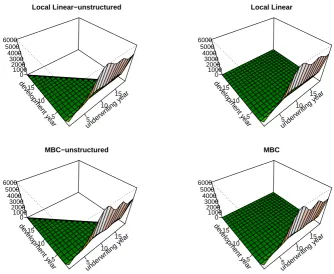
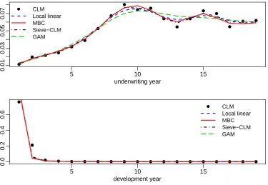
to oversmooth in the underwriting direction but undersmooth in the devel-opment component. These unstructured estimators are the starting point of our density estimator for forecasting purposes. They have been plotted in the left panels of Figure 2. The estimated densities in the underwriting and development directions (f1 and f2) are shown in Figure 3 and compared

with classical approaches such as classical chain ladder and two smoothing methods suggested in the classical reserving framework. These methods were described in Section 4 and we have focus in this application in two of them: a sieves method to smoothing the chain ladder parameters estimated from quarterly data (Verrall 1996 (check??)) and the following generalized addi-tive model (GAM) suggested by England and Verrall 1991:

log (E[Nij]) =sθi(i) +sθj(j), (14)

with sθi and sθj being smoothing splines with crossvalidated smoothing

pa-rameter. The resulting components are shown in Figure 3 and compared with the derived using the density approach and classical chain ladder.

5.3

Prediction of the outstanding claims

numbers are obtained just by summing the predicted values for the claims in the lower triangle. Thus the predicted reserves for the future calendar period are derived just by summing up the diagonals in the lower triangle i.e.

b

Dk = m X

i=2 b

Ni,m+k−i+1 = m X

i=2 b

αiβb_m+k−i+1 (15)

for k = 1, . . . , m−1. Thus the overall total will be R = Pm−q

t=1 Dt. Under

the continuous approach these predictions are defined from the following integrals:

b

Dt=τ Z T

0 b

f1(x)fb₂(T −x+t)dx, (16)

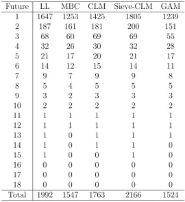
for calendar timet+T witht ∈(0, T). Hereτ is the total exposure inI. The predictions derived from the classical CLM and the continuous approach (LL and MBC) are reported in Table 1. The results are compared also with the classical chain ladder projections and the two smoothing methods in classical reserving defined above.

We can see that the compared method are quite different so the natural question is to perform a validation of the methods for the analyzed data set. This is our aim in the next subsection but before moving there just to point out that the performance of the methods should be asses for different prediction goals. This is the best method to predict individual data (in this case cells in the yearly triangle) could not be the best when the aim is to predict an aggregation of the claims such as calendars or the overall total. In fact, using the smoothing ideas in this paper to predict cells should be required an undersmooth degree but the opposite will be required when the aim is to predict a total. Therefore we expect that smoothing methods works better to predict calendar years and total number of claims.

5.4

Validation

A common method used in reserving to validate the methods consists of testing against the experience. This is done through the so called backtest. The idea is quite simple: since we can only check the predictions with what we have already observed, then we simply reduce the data to estimate and use only the older data to predict the more recent data. Note that this process uses the key assumption that the past is a good predictor of the future.

1, . . . , m−c, i+j−1≤m−c}. Now we can project from this reduced triangle in the future which is given by the set Jc = {(i, j);i = 2, . . . , m−c, j =

m−c−i+ 1, . . . , m−c}. And finally we compare the projections with the original kept data which spread out in Jec={(i, j)∈ Jc;i+j−1≤m}.

We use a number of different measures for the error depending on which is the objective of prediction. Thus we are interested in validating the methods to achieve three possible aims:

1. To predict individual cells i.e. number of claims which incurred in the year i and will be reported with j−1 years of delay, Nij.

2. To predict cash flows i.e. total number of claims which will be reported in the calendar year t=i+j−1, this is Dt;c=

P

i,j:i+j−1=t,(i,j)∈JecNij.

3. And to predict the overall total of claims in the futureRc= P

(i,j)∈JecNij.

Therefore the performance of the methods applied in previous section to the data set should be evaluated in three different ways, depending on the prediction goal defined above.

Cells: Rerrc₁ =

P

(i,j)∈Jec(Nbij −Nij) 2

(i, j)∈JecNij2

(17)

Calendar: Rerrc₂ =

Pc

t=1(Db_t;c−D_t;c)2 Pc

t=1(Dt;c)2

(18)

Total: Rerr₃c= |Rbc−Rc|

Rc

(19)

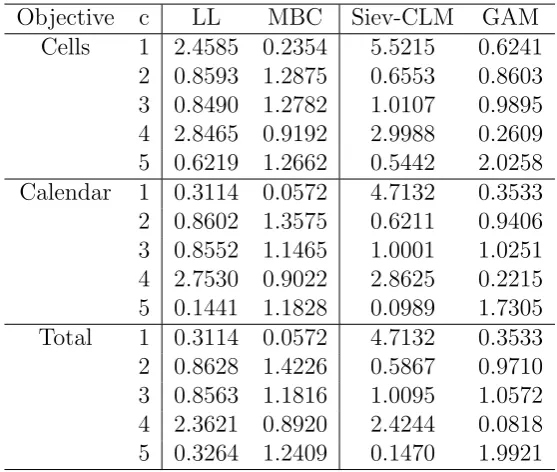
The results for the backtest projecting from the reduced trianglesJcwith

c= 1,2,3,4 and 5 years are reported in Table 2. The results from the test are quite unstable and do not provide a clear picture of which method is working better for the problem. In the next section we perform also a simulation study to provide clearer conclusions.

6

Simulation study

To do... We will simulate monthly data.

7

Conclusions

References

Bj¨ırkwall, S., H¨ıssjer, O., Ohlsson, E. and Verral, R.J. (2011), A generalized linear model with smoothing effects for claims reserving, Insurance: Mathematics and Economics, 49, 27–37.

England, P.D. and Verrall, R.J. (2001), A flexible framework for stochastic claims reserving,Proceedings of the Casualty Actuarial Society LXXXVIII, 1–38.

England, P.D. and Verrall, R.J. (2002), Stochastic claims reserving in gen-eral insurance, British Actuarial Journal, 8(3), 443–518.

Geman, S. and Hwang, C-R. (1982), Nonparametric maximum likelihood estimation by the method of sieves,Annals of Statistics, 10(2), 401–414.

Jones, M.C. (1989) Discretized and Interpolated Kernel Density Estimates,

Journal of the American Statistical Association, 84 (407) 733–741

Linton, O. and Nielsen, J.P. (1998) An optimization interpretation of inte-gration and backfitting estimators for separable nonparametric models,

Journal of Royal Statistical Society, Series B 60, 217–222.

Linton, O. and Nielsen, J.P. (1995) A kernel method of estimating struc-tured nonparametric regression, Biometrika, 82, 93–100.

Kuang, D., Nielsen B. and Nielsen J.P. (2009) chain ladder as Maximum Likelihood Revisited. Annals of Actuarial Science 4, 105–121.

Mammen,E., Linton, O. and Nielsen, J.P. (1999) The existence and asymp-totic properties of a backfitting algorithm under weak conditions, An-nals of Statistics, 27, 1443–1490.

Marx, B.D. and Eilers, P.H.C. (1998) Direct generalized additive modeling with penalized likelihood, Computational Statistics & Data Analysis, 28, 193–209.

Nielsen, J.P. (1999) Multivariate Boundary Kernels from Local Linear Es-timation, Scandinavian Actuarial Journal, 1, 93–95.

R Development Core Team (2006). R: A Language and Environment

for Statistical Computing. Vienna: R Foundation for Statistical Com-puting.

Verrall,R.J. (1989), A state space representation of the chain ladder linear model, Journal of the Institute of Actuaries, 116, 589–609.

Verrall, R.J. (1991), Chain ladder as Maximum Likelihood, Journal of the Institute of Actuaries, 118, 489–499.

Verrall, R.J. (1996), Claims reserving and generalized additive models, In-surance: Mathematics and Economics, 19, 31–43.

Verrall, R.J. (2004), A Bayesian generalized linear model for the Bornhuetter-Ferguson method of claims reserving, North American Actuarial Jour-nal, 8(3), 67–89.

W¨uthrich, M. and Merz, M. (2008). Stochastic Claims Reserving Methods in Insurance. Wiley.

Yu, K., Park, B.U. and Mammen, E. (2008) Smooth backfitting in general-ized additive models, Annals of Statistics, 36, 228–260.

Zehnwirth, B. (1989), Regression methods -applications. In: Conference Paper. 1989, Casual Loss Reserve Seminar. Available online at:

http://www.casact.org/pubs/CLRSTrans/1989/825pdf.

A

Smoothing the multiplicative density from

aggregated data

we also suggest for the density problem can be reformulated in terms of the nonparametric regression model by Linton and Nielsen (1994).

The regression formulation becomes more intuitive and at the moment more popular in the current reserving practice as we discussed in Section 4. We think that this section will be a bridge to connect with the classical reserving audience and at the same time a simple statistics exercise consisting in adapting continuous methods to practical problems where the data are given at some level of aggregation.

Let consider here the reserving problem to be solved from aggregated data into a run-off triangle such as the counts triangle, ℵm. As we describe

in Section 2.1 The regression model for the underlying problem can be written by

Nij =r(zij) +εij (20)

with zij = (xi, yj) the points in the grid, for (i, j) ∈ Im. In this case the

local linear estimator of the unstructured density resulting from solving the problem (5), for any given point z0 = (x0, y0) can be derived from the close

minimization regression problem:

b

Ψ0 b

Ψ1 !

= arg min X

(i,j)∈Im h

Nij −Ψb0 −Ψb11(x0−xi)−Ψb12(y0−yj) i2

Kh(zij−z0)dz.

(21) The solution Ψb0 gives an estimator for r(z0). By denoting as er(z0) such

estimate, the density f(z0) can be estimated by the discrete approximation

e

f(z0) =re(z0)/nΛ 2

m, (22)

with n = P

(i,j)∈ImNij and Λm the grid length. From arguments given in

Section 3.1 we can see that the estimator in (22) is equal to the local linear density estimator in (5) as the grid-length Λm goes to 0. To derive the

corresponding discrete approximation form the structured (multiplicative) density we carry out the the two-step method formulated in Section 3.3 from the just derived estimator (22).

Similarly we can derive the second improved smoother using bias reduc-tion techniques that was proposed in Secreduc-tion 3.4. Again from the above regression view we can define the multiplicative bias correction estimator as was introduced by Linton and Nielsen (1994) for nonparametric regression. The unstructured MBC estimator at any point z0 is defined from the local

linear regression estimator r_e(z0) by:

e

where eh is the local linear regression estimator calculated from a problem

like (21) but using as responses the estimates{Nij/er(zij),(i, j)∈ Im}. From

the MBC estimator _erM BC the discrete unstructured MBC density is given

by fe_{M BC}(z₀) = _er_{M BC}(z₀)/nΛ2_m. And finally we use the two-step method to

Observed counts: Nij

1234 5678

91011 121314

151617 1819 1 2 3 4 5 6 7 8 9 10 11 12 13 14 15 16 17 18 19 0 1000 2000 3000 4000 5000 i j 0 1000 2000 3000 4000 5000

Chain Ladder projections: N^ij

1234 5678

91011 121314

[image:26.595.157.481.133.637.2]

151617 1819 1 2 3 4 5 6 7 8 9 10 11 12 13 14 15 16 17 18 19 0 1000 2000 3000 4000 5000 i j 0 1000 2000 3000 4000 5000

[image:27.595.128.463.214.488.2]

underwr iting y ear 5 10 15 de velopment y ear5 10 15 0 1000 2000 3000 4000 5000 6000 Local Linear−unstructured underwr iting y ear 5 10 15 de velopment y ear5 10 15 0 1000 2000 3000 4000 5000 6000 Local Linear underwr iting y ear 5 10 15 de velopment y ear5 10 15 0 1000 2000 3000 4000 5000 6000 MBC−unstructured underwr iting y ear 5 10 15 de velopment y ear5 10 15 0 1000 2000 3000 4000 5000 6000 MBC

Figure 2: Forecasts for motor data using the continuous density approach. Left panels show the unstructured local linear (LL) and multiplicative bias corrected (MBC) estimators. The bandwidth parameters were chosen us-ing crossvalidation that provided values (h1, h2) = (10.2,2.9) for LL and

(h1, h2) = (10,3.3) for MBC. The estimated densities have been evaluated

5 10 15

0.01

0.03

0.05

0.07

underwriting year CLM

Local linear MBC Sieve−CLM GAM

5 10 15

0.0

0.2

0.4

0.6

development year

[image:28.595.110.486.235.494.2]

CLM Local linear MBC Sieve−CLM GAM

Figure 3: Estimated underwriting and development densities for motor data: incurred counts triangle. Top panel shows the resulting underwriting density (f1) from LL and MBC. Similarly for the development density (f2) in the

Future LL MBC CLM Sieve-CLM GAM 1 1647 1253 1425 1805 1239 2 187 161 181 200 151

3 68 60 69 69 55

4 32 26 30 32 28

5 21 17 20 21 17

6 14 12 15 14 11

7 9 7 9 9 8

8 5 4 5 5 5

9 3 2 3 3 3

10 2 2 2 2 2

11 1 1 1 1 1

12 1 1 1 1 1

13 1 0 1 1 1

14 1 0 1 1 0

15 1 0 0 1 0

16 0 0 0 0 0

17 0 0 0 0 0

18 0 0 0 0 0

[image:29.595.161.432.215.510.2]

Total 1992 1547 1763 2166 1524

Objective c LL MBC Siev-CLM GAM Cells 1 2.4585 0.2354 5.5215 0.6241

[image:30.595.159.438.223.459.2]

2 0.8593 1.2875 0.6553 0.8603 3 0.8490 1.2782 1.0107 0.9895 4 2.8465 0.9192 2.9988 0.2609 5 0.6219 1.2662 0.5442 2.0258 Calendar 1 0.3114 0.0572 4.7132 0.3533 2 0.8602 1.3575 0.6211 0.9406 3 0.8552 1.1465 1.0001 1.0251 4 2.7530 0.9022 2.8625 0.2215 5 0.1441 1.1828 0.0989 1.7305 Total 1 0.3114 0.0572 4.7132 0.3533 2 0.8628 1.4226 0.5867 0.9710 3 0.8563 1.1816 1.0095 1.0572 4 2.3621 0.8920 2.4244 0.0818 5 0.3264 1.2409 0.1470 1.9921