City, University of London Institutional Repository
Citation
: Zhao, Shouqi (2014). Dependent Risk Modelling and Ruin Probability:
Numerical Computation and Applications. (Unpublished Doctoral thesis, City University London)This is the accepted version of the paper.
This version of the publication may differ from the final published
version.
Permanent repository link:
http://openaccess.city.ac.uk/13702/Link to published version
:
Copyright and reuse:
City Research Online aims to make research
outputs of City, University of London available to a wider audience.
Copyright and Moral Rights remain with the author(s) and/or copyright
holders. URLs from City Research Online may be freely distributed and
linked to.
Dependent Risk Modelling
and Ruin Probability:
Numerical Computation and
Applications
Shouqi Zhao
Faculty of Actuarial Science and Insurance Cass Business School, City University London
A thesis submitted for the degree of
Doctor in Philosophy
THE FOLLOWING PREVIOUSLY PUBLISHED PAPERS HAVE BEEN
REDACTED FOR COPYRIGHT REASONS:
pp15-73:
Chapter 2
Dimitrova D.S., Kaishev V.K. & Zhao S. (2014) On the evaluation of finite-time ruin probabilities in a dependent risk model. Applied Mathematics and Computation,275, 268-286.
Abstract available from http://onlinelibrary.wiley.com/doi/10.1046/j.1365-2850.2003.00300.x/abstract (Accessed 23 December 2015)
pp135-187:
Chapter 4
Dimitrova D.S., Kaishev V.K. & Zhao S. (2014) On finite-time ruin probabilities in a generalized dual risk model with dependence. European Journal of Operational Research, 242(1), 134-148. Abstract available from http://www.sciencedirect.com/science/article/pii/S037722171400811X
(Accessed 23 December 2015)
pp191-249:
Chapter 5
Dimitrova D.S., Kaishev V.K. & Zhao S. (2015) Modeling Finite-Time Failure Probabilities in Risk Analysis Applications. Risk Analysis, 35(10), 1919-1939.
Contents
Acknowledgments xi
Declaration A xiii
Declaration B xv
Abstract xvii
1 Introduction 1
1.1 Chapter summaries . . . 5 1.2 Publications arising from this thesis . . . 9
2 On the evaluation of finite-time ruin probabilities in a
de-pendent risk model 13
2.1 Introduction . . . 15 2.2 Preliminaries . . . 18 2.3 Connections between the non-ruin probability formulas . . 23 2.4 On Appell polynomials . . . 29 2.5 A method for computingP(T > x) with a prescribed accuracy 32 2.5.1 Truncating from above . . . 33 2.5.2 Truncating from below . . . 36 2.6 A simulation-based method for computing the high
dimen-sional integrals/sums in P(T > x) with order statistics . . 38 2.6.1 The case of continuous claim amounts . . . 38 2.6.2 The case of discrete claim amounts . . . 40 2.7 Numerical study . . . 43 2.7.1 Computing the classical Appell polynomials . . . . 44 2.7.2 Comparing formulas (2.5) and (2.9), (2.4) and (2.8) 46 2.7.3 Computing P(T > x) with a prescribed accuracy . 50 2.7.4 On the simulation-based method for computingP(T >
2.10 Appendix A . . . 64
2.11 Appendix B . . . 66
3 Early warning of bankruptcy and risk capital allocation based on the time to ruin and the deficit at ruin 75 3.1 Introduction . . . 77
3.2 Alarm times and alarm systems . . . 80
3.2.1 Definition of an alarm time . . . 80
3.2.2 Explicit expressions forP(T > x) andP(T < x, Y > y) . . . 85
3.2.3 Sensitivity analysis . . . 91
3.2.4 A system with multiple alarms . . . 95
3.3 Capital allocation strategies . . . 98
3.3.1 Capital allocation strategy in a system with a single alarm time . . . 100
3.3.2 Capital allocation strategy in a system with two alarm times . . . 104
3.4 Concluding remarks . . . 106
3.5 Appendix . . . 110
4 On finite-time ruin probabilities in a generalized dual risk model with dependence 133 4.1 Introduction . . . 135
4.2 The probability of non-ruin in the dual risk model . . . 140
4.2.1 Exponential capital gains . . . 145
4.2.2 Erlang capital gains . . . 147
4.2.3 Arbitrarily distributed capital gains . . . 149
4.2.4 Linear combination of exponential capital gains . . 150
4.2.5 Dependence between capital gains, inter-arrival times and across . . . 153
4.2.6 Capital allocation and alarm time . . . 156
4.3 Numerical study . . . 161
4.4 Concluding remarks . . . 175
4.5 Appendix . . . 177
5 Modelling finite-time failure probabilities in risk analysis applications 189 5.1 Introduction . . . 191
5.2 The risk modelling framework . . . 196
5.2.1 Model A . . . 197
5.2.2 Model B . . . 202
5.3 Risk analysis applications . . . 205
5.3.2 Inventory management risk . . . 209
5.3.3 Control of flood risk via dam management . . . 211
5.3.4 Risk of emerging disease (ED) spread losses . . . . 223
5.3.5 Risk of financial ruin and insolvency . . . 225
5.4 Discussion and conclusion . . . 227
5.4.1 On infinite-time horizon . . . 227
5.4.2 On early warning measures . . . 227
5.4.3 Concluding remarks . . . 228
5.5 Appendix A . . . 230
5.6 Appendix B . . . 234
6 Conclusions 251 6.1 Summary . . . 251
List of Tables
2.1 Computation times (in sec) for P(T > x) using formula (2.9) with the assumptions of Example 2.7.1 and parameter values λ= 1, α= 0.5, c= 1.25, x= 10. . . 46
2.2 Computation times (in sec) for P(T > x) using formula (2.5) with the assumptions of Example 2.7.1 and parameter values λ= 1, α= 0.5, c= 1.25, x= 10. . . 46
2.3 Comparing the computational efficiency and accuracy of for-mulas (2.4) and (2.8) on the basis of Example 2.7.2 with parameter values λ= 1, α= 0.5, u= 1, x= 1. . . 49 2.4 The truncating points, l∗ and m∗, estimated using (2.19)
and (2.18) with k∗ = 0. . . 51
2.5 The truncating points, l∗ and m∗, estimated using (2.19) and (2.17) with k∗ = 0. . . 51 2.6 The truncating point from above in (2.4),m∗, estimated
us-ing (2.17) with varyus-ingk∗ and = 10−3, under the
assump-tions of Example 2.7.2 with parameter values λ = 1, α = 0.5, u= 1, c = 1.25, x= 1. . . 52
2.7 The truncating point from above in (2.4),m∗, estimated us-ing (2.17) withk∗ = 2 and varying, under the assumptions of Example 2.7.2 with parameter values λ= 1, α = 0.5, u= 1, c= 1.25, x= 1. . . 52
3.1 Alarm timetAwithb= 0.25 andy= 0, for differentaandd,
based on Example 3.2.3. Parameter values: λ= 2, α= 0.7,
u0 = 10 and c= 1. . . 92
3.2 Alarm time tA with b = 0.25 and y = 0.2, for different a
and d, based on Example 3.2.3. Parameter values: λ = 2,
α= 0.7, u0 = 10 and c= 1. . . 92
3.3 Alarm time tA with b = 0.25 and y = 0.5, for different a
and d, based on Example 3.2.3. Parameter values: λ = 2,
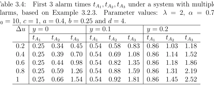
3.4 First 3 alarm timestA1, tA2, tA3 under a system with multiple
alarms, based on Example 3.2.3. Parameter values: λ = 2,
α= 0.7, u0 = 10, c= 1, a = 0.4,b = 0.25 and d= 4. . . 97
4.1 Parameters of the hyperexponential cdfH4(z), fitted to Pareto(1.2,5),
applying the algorithm of Feldmann and Whitt (1998). . . 163 4.2 Parameters of H4(z), fitted to Weibull(0.6,0.66464),
apply-ing the algorithm of Feldmann and Whitt (1998). . . 165 4.3 Survival probability and computation times using
formu-las (4.8) and (4.15). Parameter values g = 3 and λi =
1,1,1 2,
1
2, . . . for i = 1,2, . . ., α = 2, β = 0.5, U0 = 1, x = 2
List of Figures
2.1 Computation times (in sec) for P(T > x) using formula (2.5) - blue (solid) line, and formula (2.9) - red (dashed) line, with the assumptions of Example 2.7.1 and parameter values λ= 1, α= 0.5, c= 1.25. . . 47 2.2 The absolute bias of the simulated estimates of P(T > x)
(left panels) and their corresponding variances (right pan-els) using both the order statistics simulation-based method (red solid line) and direct MC simulation (blue dashed line), obtained with the assumptions of Example 2.7.1. Parameter values: λ = 1, c = 1, = 10−4, l∗ = 0, m∗ = 15 (n = 15) and M = 100. . . 55
2.3 The absolute bias of the simulated estimates of P(T > x) (left panels) and their corresponding variances (right pan-els) using both the order statistics simulation-based method (red solid line) and direct MC simulation (blue dashed line), obtained with the assumptions of Example 2.7.1. Parameter values: λ = 1, c = 1, = 10−4, l∗
= 0, m
∗
= 15 (n = 20)
and M = 100. . . 56 2.4 The absolute bias of the simulated estimates of P(T > x)
(left panels) and their corresponding variances (right pan-els) using both the order statistics simulation-based method (red solid line) and direct MC simulation (blue dashed line), obtained with the assumptions of Example 2.7.2. Parameter values: λ= 1, c= 1, = 10−4, l∗ = 0, m∗ = 15 and M = 100. 58 2.5 The simulated estimates ofP(T > x) (left panels) and their
corresponding variances (right panels) using both the or-der statistics simulation-based method (red solid line) and direct MC simulation (blue dashed line), obtained with the assumptions of Example 2.7.3. Parameter values (a): λ= 1,
c= 3, = 10−6, l∗
= 0, m
∗
= 9 and M = 100. Parameter
values (b): λ = 1, c = 1, = 10−4, l∗
3.1 Alarm timetAagainst dependence levelθ, based on Example
3.2.4. Parameter values: λ = 1, α = 5, β = 2, c= 10, a = 0.4, b = 0.1, d = 2 and y = 0.5. Blue (solid), red (dotted) and brown (dashed) lines representu0 = 5,6,7 respectively. 94
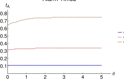
3.2 First 3 alarm timestA1, tA2, tA3 under a system with multiple
alarms, based on Example 3.2.4. Parameter values: λ = 1,
α = 5, β = 2, u0 = 5, c = 10, ∆u = 1, a = 0.4, b = 0.03,
d = 2 and y = 0.5. Blue (solid), red (dotted) and brown (dashed) lines represent alarm times 1, 2, 3, respectively. . 98
3.3 Alarm time tA for varying choices of initial capital u0.
Pa-rameter values: λ = 2, α = 0.7, u = 10, c = 1, a = 0.4,
b= 0.25 and d= 3. . . 102
3.4 Survival probability P(T > x) against different levels of initial capitalu0. Parameter values: λ= 2, α= 0.7,u= 10,
c = 1, a = 0.4, b = 0.25 and d = 3. Blue (solid) and red (dotted) lines represent r= 5% and r = 10% respectively. . 103
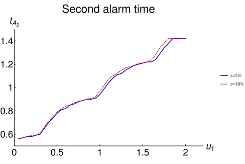
3.5 The second alarm time tA2 for different values of u1.
Pa-rameter values: λ = 2, α = 0.7, u0 = 10, u0 = 2, c = 1,
a = 0.4, b = 0.25 and d = 4. Blue (solid) and red (dotted) lines represent r= 5% and r= 10% respectively. . . 106
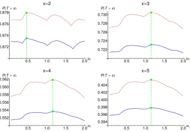
3.6 Survival probability P(T > x) against different choices of
u1. Parameter values: λ = 2, α = 0.7, u0 = 10, u0 = 2,
c = 1, a = 0.4, b = 0.25 and d = 4. Blue (solid) and red (dotted) lines represent r= 5% and r = 10% respectively. . 107
4.1 Ruin under the dual risk model vs. ruin under the insurance risk model. . . 144
4.2 Cdf of Pareto(1.2,5) vs. cdfH4(z) of fitted hyperexponential
distribution . Blue (solid) and red (dotted) lines represent cdf’s of the original and fitted distribution respectively. . . 164
4.3 Cdf of Weibull(0.6,0.66464) vs. cdf H4(z) of fitted
hyperex-ponential distribution . Blue (solid) and red (dotted) lines represent cdf’s of the original and fitted distribution respec-tively. . . 165
4.4 Survival probability againstα for Erlang capital gains with a randomized rate parameter Λ and exponential inter-arrival times using formula (4.16). Parameter values g = 3, β = 3,
θ = 1.5, c = 0.6, x = 2, = 10−5 and m
= 4. Blue
(solid), red (dashed) and purple (dotted) lines represent
4.5 Survival probability against γ for Erlang capital gains with a randomized rate parameter Λ and exponential inter-arrival times with a randomized parameter Θ and the dependence between Λ and Θ modelled by an FGM copula, using formula (4.17). Parameter values g = 3, αλ = 2, βλ = 3, αθ = 2, βθ = 0.5,c= 0.6, x= 2, = 10−5 and m= 4. . . 170
4.6 Comparing alternative strategies of capital allocation. Left panel: two choices ofhdual(t),h1(t) =−0.777+0.5t(blue/solid)
and h2(t) = (−0.577 + 0.491t)I{0≤t<1.1}+ (−0.577 + 0.491∗
1.1−0.2+0.511(t−1.1))I{1.1≤t≤2} (red/dashed). Right panel:
P(Tdual > 2) as a function of the location tJ of the capital
injection inh2(t) of sizeJ = 0.2. Parameter values: λ= 0.1,
θ= 3, = 10−6 and m = 3. . . 172
4.7 Alarm times A against U0 and c, computed according to
definition (4.20), or occasionally (4.21), following the nu-merical procedure introduced in Section 4.2.6. Parameter values α = 0.5, β = 0.05, d = 2, λ = 2 and θ = 1. Left panel: blue (solid), red (dashed) and purple (dotted) lines represent c = 0.5,0.6,0.7 respectively. Right panel: blue (solid), red (dashed) and purple (dotted) lines repre-sentU0 = 0.8,1.0,1.2 respectively. . . 174
5.1 Model A. In the left panel, h(t) (red/linear line) represents the deterministic upper critical level andS(t) (blue/staircase line) is the stochastic loss process. In the right panel, R(t) is the risk process. . . 199
5.2 Model B. In the left panel, hdual(t) (red/linear line) repre-sents the lower risk level bound and S(t) (blue/staircase line) is the stochastic gain process. In the right panel, R(t) is again the risk process. . . 204
5.3 A connection between model A and model B. . . 204
5.4 Left panel: two possible candidates h1(t), h2(t)∈ H. Right
panel: P(T > x) as a function of the location tJ of the
jump of sizeJ. Parameter values: λ= 5, α= 0.1, u= 12.5,
c1 = 3, x= 2, J = 2.5 and = 0.01. . . 208
5.6 The probabilitiesP(Tc< x) (solid lines) and P(Tc< x, Y > H−h) (dashed lines) against varying x. Left panel: expo-nential water inflow severities with parameter valuesλ= 10 and α = 0.2. Right panel: Pareto water inflow severities with parameter values λ = 1, β = 50 and θ = 2. Other parameter values: H = 100, h1 = 0.8H (blue lines) and
h2 = 0.9H (red lines). . . 216
5.7 A direct strategy of dam management where water is re-leased instantaneously at the time instants when the pre-specified critical thresholdh is exceeded. . . 217 5.8 A probabilistic strategy of dam management incorporating
an early warning signalling for water releases based on the exceedance probability P(Tc< t). . . 219
Acknowledgments
This PhD research project was funded by way of a bursary from the Faculty of Actuarial Science and Insurance at Cass Business School, City University
London.
I would like to express my sincere gratitude to several key individuals
for their kind support and assistance during the period of research and
preparation of this thesis.
My first thankfulness goes to my supervisors, Prof. Vladimir K.
Kai-shev and Dr. Dimitrina S. Dimitrova. They have been doing their best to
support me in my research and their knowledgeability steers the research
in the most productive directions. Their passions for research and enthusi-asms about this topic have been the key inspiration and the main drive for
this fruitful project. I would also like to thank them for their paternalistic
care and encouragement throughout my PhD.
Second, I would like to thank the following mates for sharing their PhD
experience with me and for the joyful time we have spent together in the
PhD office, Dr. Feng Zhou, Dr. Yiou Lu, Anran Chen, Lulu Feng, Cheng
Yan, etc. I also thank many of my good friends for the happiness they
have brought me during these years in London.
I also owe my gratitude to my best friend, Jun. He has been accompa-nying me during many difficult times.
Finally, my great gratitude to my parents for their continuing care and
support. Their deep love and kind understanding is an invaluable asset for
all my life and the key drive for me to achieve a better self.
Without these individuals, this thesis would not have been possible and
Declaration A
I herewith declare that I have produced this thesis without assistance of any third parties other than the co-authors of the papers. Additionally,
without making use of aids other than those specified: notions taken over
directly or indirectly from other sources have been identified as such. This
thesis have not previously been presented in identical or similar form to
any other UK or foreign examination board.
This thesis work was conducted from October 2010 to June 2014 under
the supervision of Prof. Vladimir K. Kaishev and Dr. Dimitrina S.
Dim-itrova at Sir John Cass Business School, City University London.
Declaration B
Powers of discretion are hereby granted to the University Librarian to allow this thesis to be copied in whole or in part without further reference to the
author. This permission covers only simple copies made for study purpose,
Abstract
In this thesis, we are concerned with the finite-time ruin probabilities in
two alternative dependent risk models, the insurance risk model and the
dual risk model, including the numerical evaluation of the explicit
expres-sions for these quantities and the application of the probabilistic results
obtained. We first investigate the numerical properties of the formulas
for the finite-time ruin probability derived by Ignatov and Kaishev (2000,
2004) and Ignatov et al. (2001) for a generalized insurance risk model
allowing dependence. Efficient numerical algorithms are proposed for com-puting the ruin probability with a prescribed accuracy in order to facilitate
the following studies. We then propose a new definition of alarm time in the
insurance risk model, which generalizes that of Das and Kratz (2012),
ex-pressed in terms of the joint distribution of the time to ruin and the deficit
at ruin. The alarm time is devised to warn that the future ruin probability
within a finite-time window has reached a pre-specified critical level and
capital injection is required. Due to our definition, the implementation
of the alarm time highly relies on the computation of the finite-time ruin
probability, which utilizes the previous results on computing the ruin prob-ability with a prescribed accuracy. The results of the ruin probprob-ability and
the alarm time are then transferred nicely to a generalized dual risk model,
whose name stems from its duality to the insurance risk model, through an
enlightening link established between the two risk models. Finally, based
on the two alternative risk models, we introduce a framework for
analyz-ing the risk of systems failure based on estimatanalyz-ing the failure probability,
and illustrate how the probabilistic models and results obtained can be
ap-plied as risk analytic tools in various practical risk assessment situations,
Chapter 1
Introduction
This thesis focuses on the ruin probability within a finite time horizon in
dependent risk models and the numerical implementation and applications.
We start from insurance risk model. The classical insurance risk model
assuming independence among claim severities and claim arrivals has been
believed unrealistic and cannot meet the needs of practical risk modelling
in reality. Research on ruin probability beyond the classical risk model
has intensified significantly in recent year. More general ruin probability
models assuming dependence between claim amounts and/or claim arrivals
and non-linear aggregate premium income have been considered in the
actuarial and applied probability literature. Such models are better suited
to reflect the dependence in the arrival and severity of losses generated
by portfolios of insurance policies. Exploring ruin probability theoretically
and numerically, under these more general dependence assumptions, is of
utmost importance within the Solvency II framework of internal
insolvency-risk model building.
considered by Ignatov and Kaishev (2000, 2004) and Ignatov et al. (2001),
where the premium income function is assumed an arbitrary non-negative
non-decreasing real function of time only, and the claim amounts are
as-sumed arbitrarily distributed with any dependent structures, following a
homogeneous Poisson claim arrival process. Under such reasonably
gen-eral assumptions, we explore the explicit ruin probability formulas and
their efficient numerical implementation to facilitate the following studies,
and demonstrate that the formulas are useful not only theoretically but
also in computing ruin probabilities in the dependent risk model. The
lat-ter is important in practical applications. For example, as recently pointed
out by Das and Kratz (2012), the need to evaluate the Ignatov-Kaishev
ruin probability formulas naturally arises in the context of designing early
warning systems against ruin of insurance companies. This need also arises
in the context of reserving and risk capital allocation in particular, for
op-erational risk, see Kaishev et al. (2008).
We then propose a new definition of alarm time in the insurance risk
model, which generalizes that of Das and Kratz (2012), expressed in terms
of the joint distribution of the time to ruin and the deficit at ruin. The
key inspiration for this part of research is the idea introduced by Kaishev
et al. (2008) that, instead of locking up a significant amount of reserve
capital initially, part of it could be invested more profitably and reserved
at a later instant, without sacrificing the predetermined overall solvency
target. Kaishev et al. (2008) demonstrate that allocating capital in two
portions, one initially and one at a later instant, leads to the same (99%)
non-ruin probability as in the case of the entire capital being reserved
strategies assume equal amount of premium (and capital) accumulated
at the end of the period, but different premium rates. The approach of
Kaishev et al. (2008) has been recently extended by Das and Kratz (2010,
2012) who base their framework on the notion of alarm time. The latter is a
future time instant at which short-term ruin probability is alarmingly high
and exceeds the predetermined threshold level. The additional portion of
capital could then be reserved at the alarm time so that the probability
of ruin falls below the threshold level. It should be noted that such a
capital allocation strategy is determined at the start of the reserving period
and is reflected in the capital and future premium income function which
models the allocation of the portions of risk capital and the accumulation
of premiums over time.
Due to our newly proposed definition of alarm time, its
implementa-tion highly relies on the computaimplementa-tion of the finite-time ruin probability,
which utilizes the previous results on computing the ruin probability with
a prescribed accuracy. The new definition also involves the joint
distri-bution of the time to ruin and the deficit at ruin, motivated by the idea
that, even though the company may get ruined, the deficit at ruin may
be small, allowing the company to easily borrow and recover. Therefore,
incorporating deficit at ruin in the definition of alarm time allows one to
emphasize only ruin cases with significant deficit. We therefore derive new
expressions for the joint distribution of the time to ruin and the deficit at
ruin, under more general assumptions.
The results of the ruin probability and the alarm time in the insurance
risk model are then transferred nicely to a generalized dual risk model,
an enlightening link established between the two risk models. As noted by
Avanzi et al. (2007), while the insurance risk model is suitable for modelling
insurance risks, the dual risk model has a wider application. It describes
well the operation of companies specializing in geological exploration of
minerals and petroleum, pharmaceutical research, and technological
dis-coveries and inventions, where routine operations generate continuous
ex-penses over time and occasional discoveries or inventions bring stochastic
capital gains to the company. It can also be applied in modelling the
op-eration of research and development departments from companies in other
industries. Or alternatively, these could be banks, hedge funds or other
investment companies, receiving capital gains from their investment and
other financial operations, while at the same time experiencing
perma-nently accumulating operational expenses. Thus, the results obtained in
the dual risk model are highly applicable for modelling the insolvency of
such institutions.
Finally, we turn our attention to the practical application of the
depen-dent risk models introduced and the probabilistic results obtained in this
thesis. Based on the two alternative risk models, we introduce a
frame-work for analyzing the risk of systems failure based on estimating the
failure probability, and illustrate how the probabilistic models and results
obtained can be applied as risk analytic tools in various practical risk
as-sessment situations, such as systems reliability, inventory management,
flood control via dam management, infection disease spread and financial
1.1
Chapter summaries
This thesis is organized as a series of papers, each of which is presented
in a separate chapter. All the four chapters/papers have been submitted
to peer reviewed journals. It is worth pointing out that all the papers
are based on joint work with my PhD supervisors. In what follows, we
summarize the main results of each chapter, and a list of the publications
arising from this thesis is provided in Section 1.2.
In Chapter 2, we consider a generalized insurance risk model
assum-ing an arbitrary non-negative, non-decreasassum-ing premium income function,
possibly dependent claim severities with any dependence structures,
fol-lowing a homogeneous Poisson claim arrivals, and focus on the finite-time
ruin probability in this dependent risk model. First, we summarize the
ex-plicit ruin probability formulas which appear in the papers by Ignatov and
Kaishev (2000, 2004) and Ignatov et al. (2001) and provide their unified
treatment in terms of classical Appell polynomials. This is achieved by
es-tablishing some enlightening connections between these formulas. Second,
we consider their efficient numerical implementation, and demonstrate that
the formulas are useful not only theoretically but also in computing ruin
probabilities in the generalized insurance risk model. For this purpose, we
propose a method of computing survival probability with a prescribed
ac-curacy and introduce and examine a simulation-based method employing
order statistics proposed by Dimitrova and Kaishev (2013). Extensive
nu-merical experiments and comparisons are provided, covering cases of both
discrete and continuous, dependent and independent claim severities.
risk model, which generalizes that of Das and Kratz (2012). The insurance
risk model considered in this chapter is more general than that considered
in Chapter 2, as we here further relax the assumption of Poisson claim
arrivals. In our new definition of alarm time, we incorporate not only the
finite-time ruin probability, but also the deficit at ruin. The motivation for
this is that, even though the company may get ruined, the deficit at ruin
may be small, allowing the company to easily borrow and recover.
There-fore, incorporating deficit at ruin in the definition of alarm time allows one
to emphasize only ruin cases with significant deficit. In order to
numer-ically evaluate the alarm time in the more general insurance risk model,
we summarize existing ruin formulas and also derive some new closed-form
expressions for the joint probability of the ruin time and the deficit at ruin
under the relaxed assumptions, in terms of exponential Appell polynomials,
introduced by Ignatov and Kaishev (2012). Based on our new definition of
alarm times, we formulate an optimal dynamic capital allocation problem.
Based on its numerical solution, we demonstrate that reserving capital
se-quentially in portions at the alarm times, rather than reserving the capital
initially as a lump sum, leads to higher finite-time survival probability.
We therefore demonstrate such dynamic capital allocation strategies are
very appealing from a solvency risk management perspective. Extensive
numerical examples are also provided.
In Chapter 4, we turn our attention to the dual risk model, whose name
stems from its duality to the insurance risk model. We consider a
general-ized dual risk model assuming any non-negative non-decreasing cumulative
operational cost function and arbitrary capital gain arrival process and
consid-ered before. First, by establishing an enlightening connection between the
two models, a trajectory hitting an upper bound and a trajectory hitting a
lower bound, we link the dual risk model with its corresponding insurance
risk model. By revisiting the formulas of survival probability in two
rea-sonably general insurance risk models considered by Ignatov and Kaishev
(2004) and Ignatov and Kaishev (2012), we obtain explicit formulas for
the finite-time survival probability in our generalized dual risk model for
exponential and Erlang capital gains, in terms of classical Appell
polyno-mials and the exponential Appell polynopolyno-mials, respectively. The results
are then generalized to the case where capital gains follow a linear
combi-nation of exponential distributions or a hyperexponential distribution. The
latter result is then used to obtain the survival probability for arbitrarily
distributed capital gains, including heavy-tailed families. We further
re-lax the independence assumptions in our dual risk model and introduce
certain dependence structures between capital gains and/or inter-arrival
times in order to make the model more realistic. Finally, we address the
problem of risk capital allocation in the dual risk model, which to the best
of our knowledge, has not been previously considered in the literature.
We base our approach on the ideas of Kaishev et al. (2008) of
distribut-ing the initial capital over a finite-time horizon without affectdistribut-ing a fixed
desired sufficiently high level of survival probability in the insurance risk
model. These ideas have been further extended by Das and Kratz (2012),
who introduced the concept of alarm time, an early warning system to the
problem of risk capital allocation. In our work, we transfer these ideas and
concepts to the dual risk model and illustrate them numerically.
the two risk models considered in this thesis. Chapter 5 develops a
frame-work for analyzing the risk of systems failure based on estimating the
failure probability. The latter is defined as the probability that a certain
risk process, characterizing the operations of a system, reaches a possibly
time-dependent critical risk level within a finite-time interval. Under
gen-eral assumptions, we utilize the probabilistic results obtained in previous
chapters for the failure probability and also the joint probability of the time
of the occurrence of failure and the excess of the risk process over the risk
level. We illustrate how to interpret the model parameters of the two
alter-native risk models in order to reflect the specifics of the concrete practical
risk assessment problems and how the probabilistic results obtained can
be successfully applied in several important areas of risk analysis among
which systems reliability, inventory management, flood control via dam
management, infection disease spread and financial insolvency. Numerical
1.2
Publications arising from this thesis
Chapter 2: On the evaluation of finite-time ruin probabilities in a
depen-dent risk model.
This chapter has been submitted to a peer reviewed journal as:
Dimitrova, D.S., Kaishev, V.K., Zhao, S. 2014. On the evaluation of
finite-time ruin probabilities in a dependent risk model.
Chapter 3: Early warning of bankruptcy and risk capital allocation based
on the time to ruin and the deficit at ruin.
This chapter has been submitted to a peer reviewed journal as:
Dimitrova, D.S., Kaishev, V.K., Zhao, S. 2014. Early warning of bankruptcy
and risk capital allocation based on the time to ruin and the deficit at ruin.
Chapter 4: On finite-time ruin probabilities in a generalized dual risk model with dependence.
This chapter has been submitted to a peer reviewed journal as:
Dimitrova, D.S., Kaishev, V.K., Zhao, S. 2014. On finite-time ruin
proba-bilities in a generalized dual risk model with dependence.
Chapter 5: Modelling finite-time failure probabilities in risk analysis
ap-plications.
This chapter has been submitted to a peer reviewed journal as:
Dimitrova, D.S., Kaishev, V.K., Zhao, S. 2014. Modelling finite-time
References
Avanzi, B., H.U. Gerber, E.S. Shiu. 2007. Optimal dividends in the dual model. Insurance: Mathematics and Economics, 41, 111–123.
Das, S., Kratz, M. 2010. On devising various alarm systems for insurance
companies. IIM Bangalore Working Paper 332 and ESSEC Working
Pa-per 10008.
Das, S., M. Kratz. 2012. Alarm system for insurance companies: A strategy
for capital allocation, Insurance: Mathematics and Economics, 51(1),
53–65.
Dimitrova, D.S., V.K. Kaishev. 2013. On the infinite-time ruin and the
distribution of the time to ruin.Submitted. Paper presented at the 10th IME conference, Leuven, Belgium, July 18–20 2006.
Ignatov, Z.G., V.K. Kaishev. 2000. Two-sided Bounds for the Finite-time Probability of Ruin. Scandinavian Actuarial Journal, 2000(1), 46–62.
Ignatov, Z.G., V.K. Kaishev. 2004. A Finite-Time Ruin Probability
For-mula For Continuous Claim Severites. Journal of Applied Probability,
41(2), 570–578.
Ignatov, Z.G., V.K. Kaishev. 2012. Finite time non-ruin probability for
Er-lang claim inter-arrivals and continuous inter-dependent claim amounts.
Stochastics: An International Journal of Probability and Stochastic
Pro-cesses, 84(4), 461–485.
Ignatov, Z.G., V.K. Kaishev, R.S. Krachunov. 2001. An Improved
Finite-time Ruin Probability Formula and its ”Mathematica” Implementation.
Kaishev, V.K., D.S. Dimitrova, Z.G. Ignatov. 2008. Operational Risk and
Insurance: A Ruin-probabilistic Reserving Approach.Journal of
Chapter 2
On the evaluation of
finite-time ruin probabilities in
On the evaluation of finite-time ruin probabilities in a
dependent risk model
Abstract
This paper establishes some enlightening connections between the explicit
formulas of the finite-time ruin probability established by Ignatov and
Kai-shev (2000, 2004) and Ignatov et al. (2001) for a risk model allowing
de-pendence. The numerical properties of these formulas are investigated and
efficient algorithms for computing ruin probability with prescribed accuracy
are presented. Extensive numerical comparisons and examples are provided.
Keywords: finite time ruin probability, dependent risk modelling, Appell
Chapter 3
Early warning of bankruptcy
and risk capital allocation
based on the time to ruin and
Early warning of bankruptcy and risk capital
alloca-tion based on the time to ruin and the deficit at ruin
Abstract
We present a new definition of an alarm time, which generalizes that of Das
and Kratz (2012), and is expressed in terms of the joint distribution of the
ruin time and the deficit at ruin under a general insurance risk model with
dependence. In order to evaluate the alarm time, we summarize existing
ruin formulas and also derive some new closed-form expressions for the joint
probability of the ruin time and the deficit at ruin, in terms of exponential
Appell polynomials, introduced by Ignatov and Kaishev (2012b). Based
on our new definition of alarm times, we formulate an optimal dynamic
capital allocation problem. Based on its numerical solution, we demonstrate that reserving capital sequentially in portions at the alarm times, rather
than reserving the capital initially as a lump sum, leads to higher
finite-time survival probability. We therefore demonstrate such dynamic capital
allocation strategies are very appealing from a solvency risk management
perspective. Extensive numerical examples are also provided.
Keywords: alarm time, joint distribution of the ruin time and the deficit
3.1
Introduction
Problems of allocating and managing risk capital in insurance companies
have attracted considerable attention in the actuarial science literature.
Allocating capital between different business units or lines of business has
been extensively explored (see e.g. Dhaene et al. 2003; Tsanakas 2004,
2009; Dhaene et al. 2012). Under an alternative approach (see Embrechts
and Samorodnitsky 2003; Embrechts et al. 2004), risk capital is reserved at
the start of a period, so as to ensure that the probability of the company’s
future ruin is less than a predetermined solvency target level. It can be
argued however, that instead of locking up a significant amount of reserve
capital initially, part of it could be invested more profitably and reserved
at a later instant, without sacrificing the predetermined overall solvency
target. This time-distributed (dynamic) capital allocation approach has
first been considered by Kaishev et al. (2008), who demonstrate that
al-locating capital in two portions, one initially and one at a later instant,
leads to the same (99%) non-ruin probability as in the case of the entire
capital being reserved at the start of the period. In order to have a fair
comparison, the two strategies assume equal amount of premium (and
cap-ital) accumulated at the end of the period, but different premium rates.
The approach of Kaishev et al. (2008) has been recently extended by Das
and Kratz (2010, 2012) who base their framework on the notion of alarm
time. The latter is a future time instant at which short-term ruin
prob-ability is alarmingly high and exceeds the predetermined threshold level.
The additional portion of capital could then be reserved at the alarm time
be noted that such a capital allocation strategy is determined at the start
of the reserving period and is reflected in the capital and future premium
income function which models the allocation of the portions of risk capital
and the accumulation of premiums over time.
A system of alarm times at which certain portions of capital should
be reserved for the purpose of reducing finite-time ruin risk is referred by
Das and Kratz (2012) as alarm system of an insurance company. The
authors have also examined the effectiveness of the proposed strategy by
numerically comparing the finite- and infinite-time ruin probabilities in
the scenarios with and without an alarm system. Their comparison
re-sults show that the model employing an alarm system provides a higher
probability of survival in a longer time horizon. Analytical bounds for
the difference between the ruin probabilities in the two cases are also
ob-tained. It is worth noting that, the alarm time, as defined by Das and
Kratz (2012), requires only the evaluation of finite-time ruin (survival)
probability. However, instead of considering analytic expressions for the
finite-time ruin probability, the authors compute it by simulation, which
may introduce significant (simulation) error in the evaluation of the alarm
time. The reason for this, as noted by the authors, is that the time unit
with which the alarm time is computed is not specified in absolute terms
and a unit of time may correspond to a long period. Therefore, a small
inaccuracy in the simulated alarm time can make a big difference in
ab-solute terms. It should also be mentioned that Das and Kratz (2012) do
not consider the problem of how much capital to allocate at each alarm
time, which is in fact the most important question in practical risk capital
This paper can be viewed as a follow-up from Das and Kratz (2012), and
our objective is four-fold. First, we propose a new definition of alarm time
which generalizes that of Das and Kratz (2012). In our new definition (see
Definition 3.2.2), we incorporate not only the finite-time ruin probability,
but also the deficit at ruin. The motivation for this is that, even though
the company may get ruined, the deficit at ruin may be small, allowing the
company to easily borrow and recover. Therefore, incorporating deficit at
ruin in the definition of alarm time allows one to emphasize only ruin cases
with significant deficit. Second, as discussed above, since simulation may
introduce significant errors, we give explicit expressions for the finite-time
survival probability and the joint probability of the time to ruin and the
deficit at ruin, which we also use to evaluate the alarm time numerically.
Explicit expressions for these two probabilities, under a reasonably general
risk model allowing dependence, are summarized in Section 3.2.2. Some
new expressions are also derived under further extensions of the model,
which is our third contribution in the paper (see Theorem 3.5.1 in the
Appendix). Our fourth contribution is related to suggesting an optimal
way of determining the amount of capital which needs to be allocated at
the alarm times as part of an alarm system for an insurance company (see
Section 3.3). We recall that such an optimal capital allocation problem
has not been considered by Das and Kratz (2012).
The paper is organized as follows. In Section 3.2.2, we introduce the
framework we are concerned with in this paper and the related assumptions
and notations. Various expressions for the finite-time survival probability
and the joint probability of the time to ruin and the deficit at ruin are
alarm time proposed by Das and Kratz (2012) in Section 3.2.1, where we
incorporate in the new definition both the ruin probability and the deficit
at ruin. We study the impacts of different parameters in the model with
ex-tensive numerical examples and parameter settings, covering both discrete
and continuous, dependent and independent claim severities. In Section
3.2.4, we devise a system with multiple alarms based on the definition of
a single alarm. Section 3.3 is devoted to studying the capital allocation
strategies in the alarm system. Optimization problems of capital
alloca-tion are formulated and attempted in simple cases with only one and two
alarms in Sections 3.3.1 and 3.3.2 respectively. Section 3.4 concludes the
paper.
3.2
Alarm times and alarm systems
In this section we introduce the concepts of alarm time and alarm system
and demonstrate how the latter can be used to allocate risk capital over
time. For the purpose we first introduce the insurance risk model and
related notation.
3.2.1
Definition of an alarm time
We start by considering the notion of alarm time, as defined by Das and
Kratz (2012), and then we provide its further generalization. Under
gen-eral insurance risk model, which has first been considered in Ignatov and
Kaishev (2000, 2004) and Ignatov et al. (2001), the possibly dependent
random variablesW1, W2, . . . denote claim severities, andY1, Y2, . . .denote
probabil-ity mass function pY1,...,Yk(y1, . . . , yk) in case Y1, Y2, . . . are discrete. Let τ1, τ2, . . . denote the claim inter-arrival times assumed independent,
iden-tically distributed random variables. We first assume τ1, τ2, . . . follow an
exponential distribution with mean 1/λ, i.e. τi ∼Exp(λ), i = 1,2, . . .,
an assumption which will later be relaxed (see Theorem 3.5.1). Thus,
the number of claims up to time t is modelled by the Poisson process
Nt = max{i : τ1 +· · ·+τi ≤ t}, t > 0. We denote by T1, T2, . . . the
arrival times of consecutive claims, i.e. Ti = τ1 +. . .+τi, i = 1,2, . . ..
Letu0 be the initial capital at time 0 and g(t) denote the cumulative
pre-mium income function of an insurance company (or a particular line of
business), which is assumed a non-negative and non-decreasing continuous
real-valued function defined onR+ withg(0) = 0. Thus,h(t) =u0+g(t) is
the cumulative capital and premium income function. For brevity, we will
refer to h(t) as the capital-premium function. It is worth mentioning that
the function h(t) may have discontinuities, resulting from e.g. lump-sum
capital injections, in which case we define h−1(z) = inf{t :h(t) ≥z}. The
insurance company’s surplus process is expressed asRt =h(t)−St, where St =YNt is the aggregate claim amount process. The instant of ruin T is
thus defined as
T := inf{t:t >0, Rt≤0},
or T = ∞ if Rt ≥ 0 for all t, and the deficit at ruin Y is defined as Y = RT+ if T < ∞. We consider a finite-time interval [0, x], and denote
byP(T > x) andP(T < x, Y > y) the probability of non-ruin in [0, x] and
the probability that ruin occurs before timexwith a deficitY exceedingy.
it incorporates jumps in the capital-premium function h(t) and therefore
allows to implement the definitions of alarm time (and capital allocation
strategies) which follow. We note that this has not been possible under the
classical insurance risk model, where h(t) is assumed continuous, strictly
linearly increasing.
We will address the following capital allocation problem. A total risk
reserve capitalu=u0+u1 of an insurance company (or a line of business)
is available at time 0. Instead of reserving the entire capital u, only part
of it, u0, is reserved initially. A second part, u1, is released (for possible
investment) and earns interest with a certain interest rater. At an
appro-priate later moment of time, say tA, the accumulated amount u1ertA will
then be reserved. The following question then arises. Given initial capital
u0 at time 0, is there a future time instant, tA > 0, before which ruin is
very unlikely, but becomes very probable shortly after, with ruin
proba-bility exceeding an alarmingly high threshold level. If tA exists, it can be
called the alarm time, at which the additional capital, u1ertA, should be
added (injected) in the capital-premium function,h(t), so as to assure that
the probability of ruin falls below a required threshold level. This approach
provides a strategy for a dynamic allocation of a total risk capital amount
u=u0+u1 in two portions,u0 initially at timet = 0, andu1 later at time
tA. It should be noted that such a strategy is determined at time 0 by
the capital-premium function h(t)≡h0(t) =u0 +g(t), which will then be
accordingly modified and becomes h1(t) = u0 +u1ertAI{t≥tA} +g(t). The
question of how to determine u0 and u1 optimally is addressed in Section
3.3. The alarm time tA has been given the following formal definition by
Definition 3.2.1 (Das and Kratz (2012)) The alarm timetA =tA(a, b, d;h0(t))
is defined as
tA = inf{t >0 :P(T ≤t+d|T > t)≥1−a and P(T > t)≥1−b}
= inf
t >0 :P(T > t)≥max1−b, 1
aP(T > t+d)
, (3.1)
where a and b are prescribed probabilities and d represents the length of a
pre-specified future time interval (window).
As noted by Das and Kratz (2012), the value of the parameter bshould
be considerably small to ensure that the probability of ruin before the alarm
time (i.e. on [0, tA]) is minimal; the value of the parameter a needs to be
moderately small (but not too small), so that the prospect of ruin within
[tA, tA+d] is realistic and a remedial action (e.g. topping up capital) will
be required; the length of the time interval d has to be moderate, neither
very small, which leaves little possibility for remedial action to be effected,
nor very large, which indicates that ruin may occur in the distant future
and there is no strong immediate likelihood of it at timetA. In fact,a and d could be inter-related.
Clearly, in order to compute the alarm time specified in Definition 3.2.1,
one only needs to be able to compute the finite-time survival probability
P(T > t). For this purpose, one can use the explicit expressions
summa-rized in Section 3.2.2 under various assumptions for the risk model
param-eters.
It is reasonable to assume, however, that in practice, when a technical
ruin occurs and the deficit at ruin is insignificant, the insurance company
Therefore, it is reasonable to incorporate the deficit at ruin in the definition
of alarm time and highlight only ruin cases with more significant deficit
at ruin. More precisely, under Definition 3.2.2 proposed below, instead
of detecting a time window [tA, tA+d] within which ruin probability is
alarmingly high (i.e. higher than a critical level b), we consider the
likeli-hood that ruin within [tA, tA+d] occurs in combination with a large deficit
at ruin Y > y, where y is a predetermined threshold level. Therefore,
this new definition is a refinement of Definition 3.2.1, which dismisses ruin
cases when the deficit at ruin is too small to cause serious concerns for the
company.
Definition 3.2.2 The alarm time tA=tA(a, b, d;h0(t), y) is defined as
tA = inf{t >0 :P(T ≤t+d, Y > y|T > t)≥1−a and P(T > t)≥1−b}
= inf{t >0 :P(T ≤t+d, Y > y)−P(T ≤t, Y > y)≥(1−a)P(T > t)
and P(T > t)≥1−b}, (3.2)
where Y denotes the deficit at ruin and y is a pre-defined threshold level.
Clearly, Definition 3.2.2 is more general and includes Definition 3.2.1
as a special case when y = 0. It is worth pointing out that the two
conditions in (3.2) may not always be fulfilled simultaneously, i.e. we may
not necessarily be able to find such a time point tA in all cases, because,
for all possible values t such that P(T > t) ≥ 1−b, the ruin probability
(jointly with the deficit at ruin) may not increase significantly within the
future time interval [t, t+d] for fixeda,d andy. In Das and Kratz (2012),
we define the alarm time in such cases as
tA= inf{t >0 :P(T > t)<1−b}, (3.3)
i.e. the alarm time is when the survival probability drops below the
pre-scribed critical level, which makes Definition 3.2.2 more comprehensible,
avoiding “no alarm” situations appearing in Tables 2 and 3 of Das and
Kratz (2012).
As can be seen from (3.2), computing the alarm time given by
Defini-tion 3.2.2 requires computing not only the finite-time survival probability,
but also the joint distribution of the time to ruin and the deficit at ruin,
P(T < t, Y > y). Explicit expressions for the latter joint distribution
un-der various assumptions for the risk model parameters will also be provided
in Section 3.2.2.
3.2.2
Explicit expressions for
P
(
T > x
)
and
P
(
T <
x, Y > y
)
In this section, we summarize the existing explicit expressions for the
finite-time survival probability and the joint distribution of the finite-time to ruin and
the deficit at ruin in the insurance risk model described in Section 3.2.1.
We also provide some explicit results for P(T > x) and P(T < x, Y > y)
under more general model assumptions. We note that in order for these
expressions to be applied to compute tA,x should be replaced by t.
Under the insurance risk model discussed in Section 3.2.1, the
interval [0, x], P(T > x), assuming continuous claim severities, has been
derived in Ignatov and Kaishev (2004),
P(T > x) = e−λx1 +
∞
X
k=1
λk
Z h(x)
0
Z h(x)
y1
· · ·
Z h(x)
yk−1
Ak(x;ν1, . . . , νk)
×fY1,...,Yk(y1, . . . , yk)dyk. . . dy1
, (3.4)
where νk =h−1(yk), and Ak(x;ν1, . . . , νk) for k = 1,2, . . . are the classical
Appell polynomials of degree k with a coefficient in front of xk equal to 1/k!, uniquely defined as
A0(x) = 1,
A0k(x;ν1, . . . , νk) = Ak−1(x;ν1, . . . , νk−1),
Ak(νk;ν1, . . . , νk) = 0, k = 1,2, . . . ,
where ν1 ≤. . .≤ νk, νi ∈ R. It can directly be seen that formula (3.4) is
also valid for discrete claim severities (see Dimitrova et al. 2013a) in which
case it takes the form:
P(T > x) = e−λx1 +
n
X
k=1
λk
n−(k−1)
X
y1=1
n−(k−2)
X
y2=y1+1
· · ·
n
X
yk=yk−1+1
Ak(x;ν1, . . . , νk)
×pY1,...,Yk(y1, . . . , yk)
, (3.5)
where n is the integer part of h(x), i.e. n=bh(x)c.
It has been illustrated by Dimitrova et al. (2013a) that formulas (3.4)
and (3.5) are computationally appealing. For details on the numerical
properties of the two formulas, we refer to Dimitrova et al. (2013a) where
Explicit expressions for the joint distribution of the time to ruin T and
the deficit at ruin Y, P(T < x, Y > y), x > 0, y ≥ 0, are obtained by
Ignatov and Kaishev (2012a), in terms of the classical Appell polynomials,
for discrete and continuous claim severities respectively given by
P(T < x, Y > y) = 1−
m−1
X
y1=1
pY1(y1)− l
X
y1=m
pY1(y1)e
−λh−1(y 1−y)
−e−λx 1−
l
X
y1=1
pY1(y1)
! + l X k=2 X Ck
pY1,...,Yk(y1, . . . , yk)
n
Bk−2 h−1(yk−1) ;ν1, . . . , νk−2
−Bk−1 h−1(yk−y) ;ν1, . . . , νk−1
o + ∞ X k=2 X Dk
pY1,...,Yk(y1, . . . , yk)
n
Bk−2 h−1(yk−1) ;ν1, . . . , νk−2
−Bk−1(x;ν1, . . . , νk−1)
o
, (3.6)
where m=byc+ 1, n=bh(x)c, l=bh(x) +yc,
Ck={(y1, . . . , yk) : 1≤y1,1 +yi−1 ≤yi, i= 2, . . . , k−1, yk−1+y≤yk < h(x) +y}, Dk = {(y1, . . . , yk) : 1≤ y1,1 +yi−1 ≤yi, i = 2, . . . , k−1, yk−1 ≤h(x) ≤
h(x) +y ≤yk <+∞} and Bk(z;ν1, . . . , νk) = e−λz
A0+λA1(z;ν1) +· · ·+λkAk(z;ν1, . . . , νk)
P(T < x, Y > y) = Z +∞
y
f(y1)dy1−
Z h(x)+y
y
e−λh−1(y1−y)f(y
1)dy1
−e−λx
Z +∞
h(x)+y
f(y1)dy1
+ ∞ X k=2 Z . . . Z Ck n
Bk−2 h−1(yk−1) ;ν1, . . . , νk−2
−Bk−1 h−1(yk−y) ;ν1, . . . , νk−1
o
f(y1, . . . , yk)dyk. . . dy1
+ ∞ X k=2 Z . . . Z Dk n
Bk−2 h−1(yk−1) ;ν1, . . . , νk−2
−Bk−1(x;y1, . . . , yk−1)
o
f(y1, . . . , yk)dyk. . . dy1, (3.7)
whereCk ={(y1, . . . , yk) : 0< y1 < . . . < yk−1 ≤yk−1+y < yk < h(x) +y}, Dk={(y1, . . . , yk) : 0< y1 < . . . < yk−1 < h(x)≤h(x) +y≤yk <+∞}and Bk(z;ν1, . . . , νk) = e−λz
A0+λA1(z;ν1) +· · ·+λkAk(z;ν1, . . . , νk)
.
It is not difficult to verify that, when y = 0, formulas (3.6) and (3.7)
coincide with (3.5) and (3.4) respectively. The proof of that is a simplified
version (special case) of the proof of Corollary 3.5.3 (see also Appendix A
in Dimitrova et al. 2014).
In what follows, we relax the assumption of Poisson claim arrivals. As a
more general case, we assume the inter-arrival times follow an independent
non-identical Erlang distribution, i.e. τi ∼Erlang(mi, λi), and a Poisson
arrival process can be viewed as a special case where mi = 1 and λi = λ.
The following explicit expression for the finite-time survival probability has
severities with an arbitrary dependence structure governing Y1, Y2, . . .,
P(T > x) =e−λ1x+
∞
X
k=1
Z
. . .
Z
0≤y1≤...≤yj(k)≤h(x)
Bk(x)f y1, . . . , yj(k)
dyj(k)· · ·dy1,
(3.8)
where j(k), k = 0,1,2, . . . , is an integer-valued function such that
m1 +. . .+mj(k) ≤k < m1+. . .+mj(k)+mj(k)+1, (3.9)
and Bk are called exponential Appell polynomials, defined recursively as
Bk(x) =λj(k−1)+1e−λj(k)+1x
Z x
h−1(y j(k))
eλj(k)+1zB
k−1(z)dz, k = 1,2, . . . ,
with B0(x) = e−λ1x. A discrete version of (3.8) can be directly deduced.
The corresponding formula for the joint distribution of the time to ruin
and the deficit at ruin, P(T < x, Y > y), is derived in the Appendix, see
formula (3.23) in Corollary 3.5.4 (see also Appendix B in Dimitrova et al.
2014), and Corollary 3.5.5 states that, wheny= 0, formula (3.23) coincides
with (3.8).
A further generalization can be made by assuming that the inter-arrival
times are independent, non-identically distributed as a linear combination
of exponential r.v.s, i.e. τi =
Pmi
j=1αijηij, where the constants αij >0 and ηij ∼Exp(λij). The latter assumption is rather general, and includes both
the Erlang and exponential assumptions on the inter-arrival time
distribu-tion as special cases. Under this general assumpdistribu-tion, the following explicit
(2013b),
P(T > x) =
∞
X
k=0
Z
. . .
Z
0≤y1≤...≤yj(k)≤h(x)
Bk(x)f(y1, . . . , yj(k))dyj(k)· · ·dy1, (3.10)
where j(k) is defined as in (3.9),
Bk(x) =θke−θk+1x
Z x
νk
eθk+1zB
k−1(z)dz, k = 1,2, . . . ,
with B0(x) = e−θ1x, θn = λij
αij, such that
Pi−1
s=1ms < n ≤
Pi
s=1ms and j = n−Pi−1
s=1ms, and 0 ≤ ν1 ≤ ν2 ≤ . . . is a sequence of real numbers
denoting
h−1(0)≤. . .≤h−1(0)
| {z }
m1−1
≤h−1(y1)≤. . .≤h−1(y1)
| {z }
m2
≤. . . ,
correspondingly. Furthermore, under these general assumptions, we derive
the joint distribution of the time to ruin and the deficit at ruin, P(T <
x, Y > y), in Theorem 3.5.1 (see expression (3.13) and its detailed proof
in Appendix 3.5), and Corollary 3.5.3 demonstrates that, when y = 0,
formula (3.13) coincides with (3.10).
It is worth mentioning that, although we only give the expressions for
continuous claim severities under the more general assumptions of
inter-arrival times, it is straightforward to obtain the form that is valid for
discrete claim amounts.
In this section, we have summarized explicit expressions for the
finite-time survival probability and the joint probability of the finite-time to ruin and
computation of alarm times defined in Definitions 3.2.1 and 3.2.2. As
mentioned previously, to avoid the inaccuracy introduced by numerical
simulations, we choose to use explicit formulas for the these quantities, in
contrast to Das and Kratz (2012), who resort on simulation. Therefore,
the explicit expressions summarized in this section will be highly important
and helpful in the numerical analysis provided next.
3.2.3
Sensitivity analysis
In what follows, we provide some sensitivity analysis of the alarm time (3.2)
against various parameters based on the following two examples, which
cover cases of discrete and continuous, dependent and independent claim
severities.
Example 3.2.3 Claim amounts follow an i.i.d logarithmic distribution
with parameter α, i.e. W ∼Log(α) with a generic p.m.f. P(W = i) =
−αi/(i ln (1−α)).
Example 3.2.4 Claim amounts are inter-dependent with Pareto marginals,
i.e. W ∼Pareto(α, β) with a generic p.d.f. f(w) = αβ(α+w)−β−1β, and
the dependence structure is modelled by a rotated Clayton copula, which
models upper tail dependence, with density
cRCl(u1, . . . , uk;θ) = θk
Γ(1/θ+k) Γ(1/θ)
k
Y
i=1
(1−ui)−θ−1 k
X
i=1
(1−ui)−θ−k+1
−1/θ−k
,
where θ∈(0,∞) denotes the dependence parameter.
Based on Examples 3.2.3 and 3.2.4 and expression (3.2), we compute
illus-trate how it varies against different parameter values. For computational
simplicity, we assume Poisson claim arrivals and a linear premium income
function g(t) = ct, where c denotes a constant premium income rate, i.e.
h0(t) = u0+ct.
Table 3.1: Alarm time tA with b = 0.25 and y = 0, for different a and d,
based on Example 3.2.3. Parameter values: λ = 2, α = 0.7, u0 = 10 and
c= 1.
d a
0.3 0.325 0.35 0.375 0.4 0.425 0.45 0.475 0.5
2.5 2.32 2.32 2.32 2.32 2.32 2.24 2.04 1.67 1.38
2.75 2.32 2.32 2.32 2.24 2.04 1.78 1.48 1.18 1.04
3 2.32 2.32 2.15 1.82 1.58 1.33 1.05 0.86 0.71
3.25 2.32 2.06 1.62 1.40 1.18 0.88 0.70 0.56 0.42
3.5 1.88 1.46 1.26 1.07 0.86 0.61 0.41 0.28 0.15
3.75 1.43 1.13 0.88 0.74 0.53 0.30 0.14 0.02 0
4 1.03 0.82 0.63 0.44 0.25 0.03 0 0 0
4.25 0.70 0.52 0.34 0.17 0 0 0 0 0
4.5 0.42 0.25 0.08 0 0 0 0 0 0
4.75 0.15 0 0 0 0 0 0 0 0
5 0 0 0 0 0 0 0 0 0
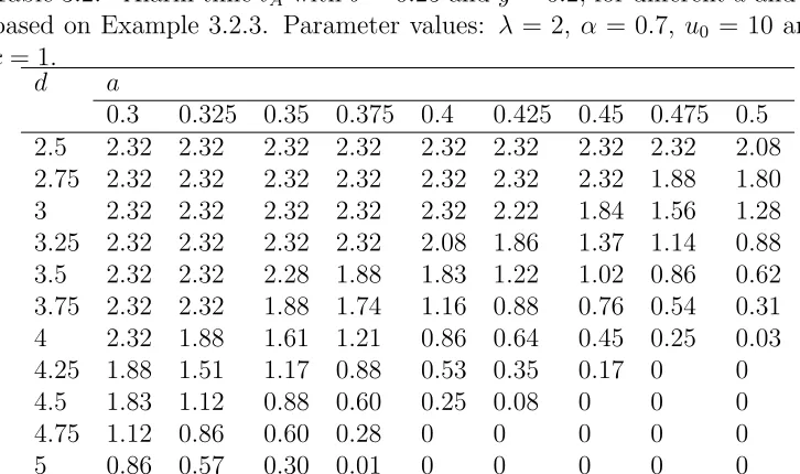
Table 3.2: Alarm timetA withb= 0.25 andy= 0.2, for differenta andd,
based on Example 3.2.3. Parameter values: λ = 2, α = 0.7, u0 = 10 and
c= 1.
d a
0.3 0.325 0.35 0.375 0.4 0.425 0.45 0.475 0.5
2.5 2.32 2.32 2.32 2.32 2.32 2.32 2.32 2.32 2.08
2.75 2.32 2.32 2.32 2.32 2.32 2.32 2.32 1.88 1.80
3 2.32 2.32 2.32 2.32 2.32 2.22 1.84 1.56 1.28
3.25 2.32 2.32 2.32 2.32 2.08 1.86 1.37 1.14 0.88
3.5 2.32 2.32 2.28 1.88 1.83 1.22 1.02 0.86 0.62
3.75 2.32 2.32 1.88 1.74 1.16 0.88 0.76 0.54 0.31
4 2.32 1.88 1.61 1.21 0.86 0.64 0.45 0.25 0.03
4.25 1.88 1.51 1.17 0.88 0.53 0.35 0.17 0 0
4.5 1.83 1.12 0.88 0.60 0.25 0.08 0 0 0
4.75 1.12 0.86 0.60 0.28 0 0 0 0 0
[image:55.522.76.439.441.656.2]Table 3.3: Alarm timetA withb= 0.25 andy= 0.5, for differenta andd,
based on Example 3.2.3. Parameter values: λ = 2, α = 0.7, u0 = 10 and
c= 1.
d a
0.3 0.325 0.35 0.375 0.4 0.425 0.45 0.475 0.5
2.5 2.32 2.32 2.32 2.32 2.32 2.32 2.32 2.32 2.32
2.75 2.32 2.32 2.32 2.32 2.32 2.32 2.32 2.32 2.32
3 2.32 2.32 2.32 2.32 2.32 2.32 2.32 2.32 2.32
3.25 2.32 2.32 2.32 2.32 2.32 2.32 2.32 2.32 2.32
3.5 2.32 2.32 2.32 2.32 2.32 2.32 2.32 2.32 1.85
3.75 2.32 2.32 2.32 2.32 2.32 2.32 2.32 1.84 1.60
4 2.32 2.32 2.32 2.32 2.32 2.32 1.88 1.61 1.12
4.25 2.32 2.32 2.32 2.32 2.32 2.16 1.75 1.10 0.81
4.5 2.32 2.32 2.32 2.32 2.32 1.82 1.53 0.81 0.55
4.75 2.32 2.32 2.32 2.32 1.88 1.61 0.83 0.56 0.23
5 2.32 2.32 2.32 2.32 1.76 1.04 0.58 0.27 0
In Tables 3.1, 3.2 and 3.3, we compare the alarm times obtained for
various choices of a, d and y, based on Example 3.2.3, where the claim
severities follow an i.i.d. logarithmic distribution. As noted by Das and
Kratz (2012), under the original definition (3.1), the alarm time decreases
with the increase of a and d, which is rather intuitive. Here, we observe
similar effects under the new definition. Particularly, for smaller values
of a and/or d, the first condition in (3.2) cannot be fulfilled prior to the
survival probability decreasing below the pre-specified level 1−b. Hence,
the alarm time is determined solely by definition (3.3) and the level of
the parameter b. In fact, b is used in order to cap the alarm time, and
its impact on tA signifies when a and d are small and definition (3.3) is
employed. It can also be observed that the alarm time increases along with
y. This is reasonable, because for a high level of the deficit threshold y, it
takes longer time t for P(T ≤ t+d, Y > y|T > t) to become significant
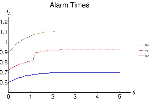
[image:56.522.78.439.116.311.2]Based on Example 3.2.4, where the claims are assumed dependent, with
a joint distribution modelled by a rotated Clayton copula with Pareto
marginals, Figure 3.1 illustrates how the alarm time varies for different
choices of the initial capital level, u0, and with the increase of the
depen-dence level, θ. Clearly, the alarm time, tA, increases with the value of u0 and also it occurs later when stronger dependence is assumed, and the
increase in tA decelerates with the increase in θ. This is because higher
level of dependence among claims, modelled by Rotated Clayton copula,
facilitates the occurrence of clusters of either small claims or large claims.
Due to the choices of the parameters, it is more likely to have a series of
small claims, which raises the survival probability and therefore defers the
alarm time,tA. With further increase in the dependence levelθ, its impact
gradually vanishes after certain level of θ and the increase in the alarm
time also diminishes.
0 1 2 3 4 5 Θ
0.6 0.7 0.8 0.9 1 1.1 1.2
tA
Alarm Times
[image:57.522.137.375.454.617.2]u0=5 u0=6 u0=7
Figure 3.1: Alarm time tA against dependence level θ, based on Example
3.2.4. Parameter values: λ = 1, α = 5, β = 2, c = 10, a = 0.4, b = 0.1,
So far, we have provided a new definition of a single alarm time,
tak-ing into account both the time to ruin and the deficit at ruin, and have
numerically illustrated the impacts of the various model parameters. In
the next section, we develop an alarm system, i.e. a system with multiple
alarm times and capital injections at each alarm time.
3.2.4
A system with multiple alarms
In this section, we introduce the concept of an alarm system, i.e. a
sys-tem with multiple alarm times and corresponding capital injections at each
alarm time. Suppose we have an initial capital u0 = h(0), which ensures
a high solvency level for the insurance company (line of business) until
time tA1, which is the first alarm time determined according to definition
(3.2). It is reasonable to suppose that the company will inject capital at
the alarm time to maintain the solvency target and keep the company
op-erational. Now, we can generalize this single-alarm time procedure and
develop a system with multiple alarms{tAi}i≥1, topping up capital at each
alarm time tAi with an amount ui. It is worth noting that all alarm times
are determined sequentially with respect to time 0, and so are the
corre-sponding capital amounts injected at each alarm time. Next, we provide
the formal definition.
Definition 3.2.5 Given the first i alarm times, tA1, . . . , tAi, and the
cor-responding capital-premium function hi(t) = u0+
Pi
k=1ui×I{t≥tAi}+g(t),
the i+ 1-th alarm time, tAi+1 =tAi+1(ai+1, bi+1, di+1;hi(t), yi+1), with