Cite as: Mackenzie, A.: A hybrid slurry CFD model. In Proceedings of CFD with OpenSource Software, 2016, Edited by Nilsson. H.,http://www.tfd.chalmers.se/~hani/kurser/OS_CFD_2016
CFD with OpenSource software
A course at Chalmers University of Technology Taught by H˚akan Nilsson
A hybrid slurry CFD model:
Euler-Euler to Euler-Lagrange
Developed for OpenFOAM-3.0.x Requires: PyFoam
Author:
Alasdair
Mackenzie
[email protected]
Peer reviewed by:
Shengnan Liu
H˚
akan Nilsson
Licensed under CC-BY-NC-SA, https://creativecommons.org/licenses/
Disclaimer: This is a student project work, done as part of a course where OpenFOAM and some other OpenSource software are introduced to the students. Any reader should be aware that it might not be free of errors. Still, it might be useful for someone who would like learn some details
similar to the ones presented in the report and in the accompanying files. The material has gone through a review process. The role of the reviewer is to go through the tutorial and make sure that
it works, that it is possible to follow, and to some extent correct the writing. The reviewer has no responsibility for the contents.
Contents
1 The problem with erosion modelling 5
2 Choosing the two solvers 6
2.1 Euler-Lagrange Model . . . 6
2.1.1 Modifying DPMFoam . . . 8
2.1.2 The 0 directory . . . 8
2.1.3 The constant directory . . . 9
2.1.4 The system directory . . . 10
2.1.5 Running the solver . . . 10
2.2 Euler-Euler Model . . . 12
2.2.1 Modifying reactingTwoPhaseEulerFoam . . . 12
2.2.2 The 0 directory . . . 12
2.2.3 The constant directory . . . 14
2.2.4 The system directory . . . 14
2.2.5 Running the solver . . . 14
3 Results from test case 16 4 Start new solver 19 4.1 Creating baffles . . . 19
4.2 Creating regions . . . 21
4.3 Create own solver . . . 22
4.4 Preparation for interpolation . . . 22
4.5 Add patchToPatchInterpolation . . . 25
5 Addition of particles to solver 28 5.1 Editing injection method . . . 28
5.1.1 Editing the KinematicLookupTableInjection folder . . . 29
5.1.2 Editing the InjectionModel folder . . . 31
5.2 Writing lookupTable in solver . . . 31
CONTENTS CONTENTS
6 Hybrid test case 36
6.1 Results . . . 37
7 Conclusions and further work 42
Learning outcomes
The reader will learn:
How to use it:
how to use an Euler-Euler dispersed phase slurry model: reactingTwoPhaseEulerFoam
how to use an Euler-Lagrange slurry model: DPMFoam
how to usecreateBaffles
how to usesplitMeshRegionsand run regions in sequence how to usepatchToPatchInterpolation
The theory of it:
the theory ofpyFoamPlotWatcher
an outline of the theory of the other utilities How it is implemented:
how to implement a new solver from two existing ones How to modify it:
Acknowledgements
I would like to acknowledge the Institute of Mechanical Engineers for their financial support for this course, which otherwise may not have been possible.
Chapter 1
The problem with erosion
modelling
Erosion caused by dense slurry flows is a common problem and computational modelling of the process is very difficult. The aim of this work is to find a more efficient way of modelling the fluid and particles, so that the erosion modelling efficiency can also be improved.
Modelling erosion of slurries using computational fluid dynamics (CFD) can be done in two ways: Euler-Euler (EE) or Euler-Lagrange (EL). The Euler-Euler technique models both the particles and fluid as continuous phases. The technique is volume averaged, and therefore not computationally expensive. Euler-Lagrange however, models particles as separate objects having their own velocity vectors. This means the particles have physical vector values near walls, which is substantially better for erosion modelling. The downside of Euler-Lagrange is that it is more computationally demanding, with varying degrees depending on one, two or four way coupling.
Chapter 2
Choosing the two solvers
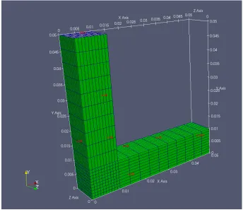
Before a hybrid model was developed, the two solvers were set up and run on a simple case, to ensure they both worked individually. A simple square-section pipe with a 90° bend was chosen, which had an inlet, outlet, and walls for boundary conditions. The geometry as seen in Figure 2.1 was taken from the tutorial by Alejandro Lopez [1], on lagrangian particle tracking. The blockMeshDict for this geometry can be found in the attached files. The pipe is 10mm square section and 100mm long, and with only 3000 cells the solution time is low. Accuracy would be improved with a finer mesh, however it is more desirable for shorter run times at this development stage. The purpose of this tutorial is not to get accurate results, but rather to develop a new model.
OpenFOAM contains various multiphase solvers and tutorials, and the idea is to find a tutorial that best matches your needs, and modify it to suit your case. Tutorials can be found by typing in the terminal window:
cd $FOAM_TUTORIALS
Or by using the alias:
tut
The standard OpenFOAM tutorials do not contain liquid/particle flow as is required; therefore the standard tutorials will need modified.
2.1
Euler-Lagrange Model
Lagrangian particle tracking uses Newton’s equations of motion to determine the particle trajectories. There are three different coupling possibilities:
one way coupled: fluid affects particles
two way coupled: as above, but particles also affect fluid
2.1. EULER-LAGRANGE MODEL CHAPTER 2. CHOOSING THE TWO SOLVERS
Figure 2.1: Geometry for test case
Two way coupling is used here since the Euler-Euler is also two way coupled. The PIMPLE solver is used for the fluid flow; the name coming from PISO-SIMPLE. PISO stands for Pressure Implicit Splitting of Operators, and SIMPLE stands for Semi-Implicit Method for Pressure Linked Equations and is used for steady state problems. This PIMPLE solver is used in combination with the kinematic cloud, to form a two way coupled algorithm. In the fvSolution dictionary, it is possible to set the number of PIMPLE loops per kinematic cloud loop by changing the variables in the PIMPLE section:
PIMPLE {
nOuterCorrectors 3; //or 2 for two loops; nCorrectors 4;
nNonOrthogonalCorrectors 4; pRefCell 0;
pRefValue 0; }
2.1. EULER-LAGRANGE MODEL CHAPTER 2. CHOOSING THE TWO SOLVERS
2.1.1
Modifying DPMFoam
The solver DPMFoam was chosen for the Euler-Lagrange simulation, as it is the most appropriate Lagrangian solver from the tutorials. Lopez [1] has shown that it can be used to model slurry flows, and more details can be found in his tutorial. The DPMFoam tutorial should be copied into the ‘run’ directory as follows:
tut
cd lagrangian
cp -r DPMFoam $FOAM_RUN run
cd DPMFoam
These commands will copy the DPMFoam tutorial from the tutorials directory to your ‘run’ directory, then open the DPMFoam folder. Typingpwdwill yield:
/home/username/OpenFOAM/username-3.0.x/run/DPMFoam
Once in this directory, the new model can be set up as shown.
2.1.2
The 0 directory
The following files should be created in the 0 directory:
0/ epsilon.water k.water nuTilda nut.water p U.water
All files in the 0 directory need to have boundary conditions assigned for each patch: in this case inlet, walls and outlet. The epsilon file is given as an example below, and all other files can be created with the same format (by copying from other tutorials), using boundary conditions that suit.
/*---*- C++ -*---*\
| ========= | |
| \\ / F ield | OpenFOAM: The Open Source CFD Toolbox |
| \\ / O peration | Version: 3.0.x |
| \\ / A nd | Web: www.OpenFOAM.org |
| \\/ M anipulation | |
2.1. EULER-LAGRANGE MODEL CHAPTER 2. CHOOSING THE TWO SOLVERS
location "0"; object epsilon; }
// * * * * * * * * * * * * * * * * * * * * * * * * * * * * * * * * * * * * * //
dimensions [0 2 -3 0 0 0 0];
internalField uniform 51;
boundaryField {
inlet {
type fixedValue; value uniform 51; }
wall {
type epsilonWallFunction; value uniform 0;
} outlet { type zeroGradient; } } // ************************************************************************* //
The value of epsilon has to be based on the inlet velocity and the geometry. The parameters used in this tutorial are as follows:
Parameter Value epsilon.water 51 k.water 0.36
nut.water 0 (no turbulent viscosity)
p 0
U.water 5
Care must be taken to ensure boundary conditions are in the correct direction, so for example ‘U’ must be(0 -5 0), i.e the negative y-direction.
2.1.3
The constant directory
The following files should be created in the constant directory, if not there already:
constant g
2.1. EULER-LAGRANGE MODEL CHAPTER 2. CHOOSING THE TWO SOLVERS
Note: blockMeshDicthas moved from OpenFOAM-3.0- onwards to the system directory, how-ever this tutorial is using some cases from OpenFOAM-2.3.x.
The ‘g’ file contains the magnitude of gravity and its direction.‘kinematicCloudProperties’ defines parameters for the lagrangian particles. Things such as velocity, density, coupling, and calculation frequency are in this dictionary. ‘RASproperties’ defines which turbulence model is used (k-epsilon in this case). The ‘turbulenceProperties’ defines the RAS turbulence model, again the k-epsilon.
2.1.4
The system directory
The following files should be created in the system directory:
system
controlDict fvSchemes fvSolution
The controlDict can be used from the DPMFoam tutorial. fvSchemes tells OpenFOAM what numerical schemes to use for each parameter, and fvSolution gives the user control over each solver for each parameter.
2.1.5
Running the solver
Once all files in their correct place, the solver can be run using the following commands:
blockMesh DPMFoam >& log&
This will first use blockMesh to mesh the domain, then start running the solver DPMFoam. The command >& log& puts error messages to the file named ‘log’, and also puts the job to the background of the terminal window. The file can be named whatever the user wishes. Typingfg
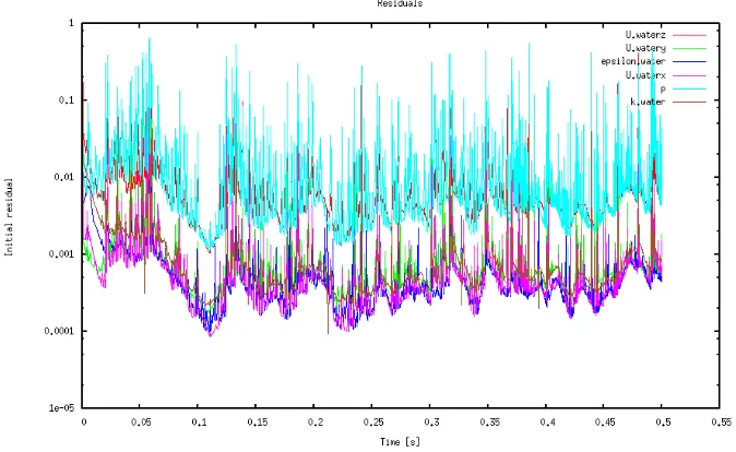
will bring the job to the foreground, so that it can be changed. Typingctr+c will cancel the job, andctrl+z will pause the job, which can be resumed in the background by typingbg. If pyFoam is installed, the application ‘pyFoamPlotWatcher’ can be used, by typing:
pyFoamPlotWatcher.py log
Wherelogis the log filename. IfpyFoamPlotWatcher.py --helpis typed, the available options for the application will be shown. The short description says:
Usage =====
pyFoamPlotWatcher.py [options] <logfile>
Gets the name of a logfile which is assumed to be the output of a OpenFOAM-solver. Parses the logfile for information about the convergence of the solver and generates gnuplot-graphs. Watches the file until interrupted.
2.1. EULER-LAGRANGE MODEL CHAPTER 2. CHOOSING THE TWO SOLVERS
Figure 2.2: Residuals from the Euler-Lagrange model
2.2. EULER-EULER MODEL CHAPTER 2. CHOOSING THE TWO SOLVERS
2.2
Euler-Euler Model
The solver reactingTwoPhaseEulerFoam was used as the Euler-Euler model. It is a solver for two compressible fluid phases with a common pressure, but otherwise separate properties. Although the two ‘fluids’ are not compressible, this can be ignored here as other models were tried and tested, but none gave results as close to the Lagrangian simulation as reactingTwoPhaseEulerFoam. twoPhaseEulerFoam was considered however the energy equation cannot be turned off in this (with-out editing the source code), which causes convergence problems.
To compare the two chosen models both were run as transient cases for 0.5 seconds real-time, with the same set-up parameters. The EE case took 684 seconds, whereas the EL took 1667 seconds; so the EE is almost 2.5 times faster than the EL for this simple case. This justifies the plan to use a hybrid model, especially when considering the time difference gets larger with more complex problems.
Note: There is a bug in myReactingTwoPhaseEulerFoam. Two files need replaced, and can be downloaded fromwww.openfoam.org/mantisbt/view.php?id=1902. The files which need replacing are ‘IsothermalModel.C/H’, and should be replaced in the folder:
$WM_PROJECT_DIR/applications/solvers/multiphase/reactingEulerFoam/phaseSystems/ phaseModel/IsothermalPhaseModel
After replacing these files, the models need to be recompiled by moving back into the ‘phaseSystems’ directory (since the ‘Make’ folder is here) and typingwclean; wmake.
2.2.1
Modifying reactingTwoPhaseEulerFoam
The fluidisedBed tutorial is to be copied in the same manner as DPMFoam was copied over to the run directory. It is found in:
.../OpenFOAM-3.0.x/tutorials/multiphase/reactingTwoPhaseEulerFoam/RAS/fluidisedBed
The folder before fluidisedBed is called RAS, indicating this is a Reynolds Averaged Simulation. Laminar or LES can also be used if required.
2.2.2
The 0 directory
The following files should be created in the 0 directory:
0/
alpha.particles alpha.water epsilon.water k.water nut.particles nut.water p
2.2. EULER-EULER MODEL CHAPTER 2. CHOOSING THE TWO SOLVERS
U.particles U.water
These should be filled in the same way as for the Euler-Lagrange simulation. For example, alpha.particles is as follows:
/*---*- C++ -*---*\
| ========= | |
| \\ / F ield | OpenFOAM: The Open Source CFD Toolbox |
| \\ / O peration | Version: 3.0.x |
| \\ / A nd | Web: www.OpenFOAM.org |
| \\/ M anipulation | |
\*---*/ FoamFile { version 2.0; format ascii; class volScalarField; object alpha.particles; } // * * * * * * * * * * * * * * * * * * * * * * * * * * * * * * * * * * * * * //
dimensions [0 0 0 0 0 0 0];
internalField uniform 0;
boundaryField { inlet { type fixedValue; value 0.039; } outlet { type zeroGradient; } walls { type zeroGradient; } } // ************************************************************************* //
2.2. EULER-EULER MODEL CHAPTER 2. CHOOSING THE TWO SOLVERS
Parameter Value
alpha.particles 0.039 (10%mass concentration) alpha.water 0.961
epsilon.water 51 k.water 0.36
nut.particles 0 (no turbulent viscosity) nut.water 0
p 1e5
Theta.particles 1e-7 (granular temperature) T.particles 300
T.water 300
U.particles 5
U.water 5
These parameters should be inserted into the appropriate dictionaries, with the boundary con-ditions required.
2.2.3
The constant directory
The following files should be created in the constant directory:
constant g
phaseProperties polyMesh
thermoPhysicalProperties.particles thermoPhysicalProperties.water turbulenceProperties.particles turbulenceProperties.water
The constant directory is similar to the DPMFoam one, but kinematicCloudProperties has been replaced with phaseProperties, and there is also thermoPhysicalProperties since there is a possibility for heat exchange to be taken into account. blockMeshDict has also moved to the ‘system’ directory.
2.2.4
The system directory
The following files should be created in the system directory:
system
blockMeshDict controlDict fvSchemes fvSolution
2.2.5
Running the solver
2.2. EULER-EULER MODEL CHAPTER 2. CHOOSING THE TWO SOLVERS
the solver:
blockMesh
Chapter 3
Results from test case
The test cases were both ran, and made sure to be similar in appearance. Again it must be re-membered that this tutorial is not about results, but rather the application of the solvers in a new way.
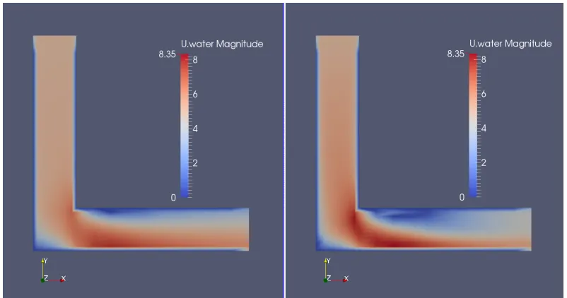
[image:17.612.95.496.383.594.2]A comparison of the water’s velocity magnitude is shown below, in Figure 3.1. This is a 2D slice, normal to the Z-plane, and shows the Euler-Lagrange on the left, and Euler-Euler on the right. It is quite clear that the velocities are similar enough to proceed. Results were taken from the last time step in all figures.
Figure 3.1: Velocity magnitude of water: EL and EE
Getting this comparison in Paraview is quite straight forward. If in the EL case folder, we need to create a case.OpenFOAM file (so that we can open it from inside Paraview). This is done by typing
touch casename.OpenFOAM
CHAPTER 3. RESULTS FROM TEST CASE
Euler-Euler folder, and type
paraFoam
This will open Paraview and automatically create a temporary file called ’casename.OpenFOAM’ (note: casename is the name of the case you have named). We can then select split screen view, and simply open the .OpenFOAM file which we created in the Euler-Lagrange folder.
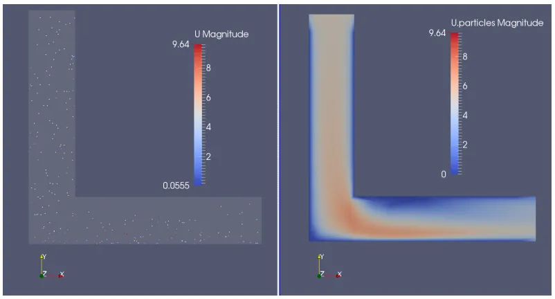
[image:18.612.95.496.277.493.2]Below in Figure 3.2 a comparison of the velocity magnitudes of the second (dispersed) phase is shown. This is slightly more difficult to compare, as one is Eulerian and the other Lagrangian, or one is continua the other particles. It can be seen that the Lagrangian particles are travelling faster than the Eulerian phase, since the Eulerian contour plot does not go as dark red as the legend does. This is because the legend has been rescaled, as the maximum velocity for the Eulerian phase was 7m/s. This difference of 2-3m/s could be down to its averaged nature, as there may only be one particle in the Lagrangian simulation that has the velocity of 9.64m/s.
Figure 3.2: Velocity magnitude of second phase: EL and EE
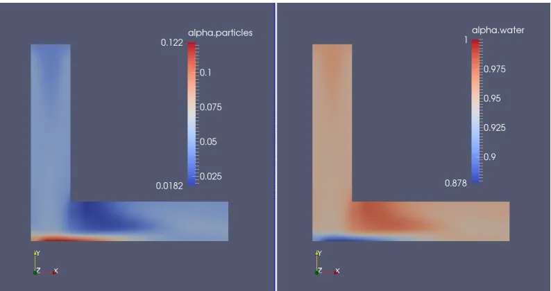
Figure 3.3 below shows the phase fractions, alpha water, and alpha particles. Alpha denotes the phase fraction of the phase name, and in every cell in the domain alpha.particles + alpha.water = 1.
CHAPTER 3. RESULTS FROM TEST CASE
Chapter 4
Start new solver
In the new hybrid model, sections of code from DPMFoam were added to reactingTwoPhaseEuler-Foam. The test domain was split into two regions, with the continuous phase running through both regions unaffected. The second (particle) phase was run as a fluid through the Euler-Euler region, and then injected as particles in the Lagrangian region, based on the Eulerian result at the interface. This should require less computational effort than if the whole domain had Lagrangian particles throughout. The steps to make this work are summarised:
Create baffles: Enable boundary conditions to be set Create regions: Enable solving regions of domain in series Add interpolator: Enable communication between regions Add DPMFoam code: Particles were added to the code
To do these things, the pipe bend case from before should be copied into a new folder, so that it can be edited to suit the new hybrid model. The new folder should be called ‘hybrid’.
4.1
Creating baffles
The square pipe was to be split into two regions, one for EE, and one for EL. There was also the requirement for having boundary conditions where the transition takes place, so that the particles injected will have the same values as the EE simulation. With these things in mind, creating baffles and then splitting the mesh into regions seemed the best option.
To create baffles, a utility file called ‘createBafflesDict’ needs to be added to the ‘system’ folder. These are already included in some tutorials; they can be found by typing:
foam
find -iname createBafflesDict
4.1. CREATING BAFFLES CHAPTER 4. START NEW SOLVER
run cd hybrid
cp ../../../OpenFOAM-3.0.x/tutorials/heatTransfer/chtMultiRegionSimpleFoam/ heatExchanger/system/air/createBafflesDict ./system/
The dictionary can be edited as required, or copied from the attached files with this report. The dictionary gives directions as to the type of baffle, and what it should be based on. In this case, making an .stl file and using it is a baffle surface is the method shown. In the dictionary, we should define the name of our .stl file next to the ‘name’ parameter. Other values can be checked in the attached case.
The .stl file now has to be made, in the constant/triSurface directory. The file in this tutorial is called ‘baffle1D.stl’, and the contents of the file are as follows:
solid ascii
facet normal 0 1 0 outer loop
vertex 0 0.01 0 vertex 0 0.01 -0.01 vertex 0.01 0.01 0 endloop
endfacet
facet normal 0 1 0 outer loop
vertex 0.01 0.01 -0.01 vertex 0.01 0.01 0 vertex 0 0.01 -0.01 endloop
endfacet endsolid
This is a simple surface, however more complex surfaces could be drawn by using any CAD software, like FreeCAD[4] for example.
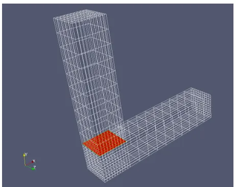
Now that the dictionary and .stl file is in place, the commands can be carried out to create the mesh and baffles, when in the ‘hybrid’ directory.
blockMesh
createBaffles -overwrite
This will create the blockMesh and also create the baffles. There will be a master and a slave patch created in each file of the 0/ directory. These patches will allow boundary conditions to be set on them, allowing a transition from Euler to Lagrangian for the second phase. The ‘overwrite’ flag ensures any previous baffles are overwritten. More information on the createBaffles utility can be found by looking at the .C file, using thefindcommand as previously described.
paraFoam
4.2. CREATING REGIONS CHAPTER 4. START NEW SOLVER
Figure 4.1: View of mesh and baffles in red
4.2
Creating regions
Now that the baffles are in place for injecting, a method of solving the regions in series is required. This is so the EE region can be solved before the EL region in the iterative loop. The utility called ‘splitMeshRegions’ can be used to split the domain into two regions along the patch line. More can be found on the utility by looking at the .C file, using the technique already provided. The following command is carried out in the working directory:
splitMeshRegions -cellZones -overwrite >log.splitMesh
-cellZones and -overwrite split the cellZones into separate regions and overwrites the existing mesh respectively. After the command is executed, a log file will be created called ‘log.splitMesh’. This should explain that two regions have been created, giving a cell count for each region, and also what each region is called. Figure 4.1 shows that the bottom region is larger than the top, and therefore is the one with more cells. If in doubt, paraview can be opened and checked which domain is which. From the log file created, domain0 has 2000 cells, whereas domain1 has 1000, therefore
domain0 is on the bottom, domain1 on top. fvSchemes and fvSolution have also been created in the system/domain(0/1) folders, enabling different schemes to be used in each region. A file called
regionProperties is made in the constant/ folder, and this is where the region type is defined e.g.
regions (
fluid (domain1) solid (domain0) );
4.3. CREATE OWN SOLVER CHAPTER 4. START NEW SOLVER
4.3
Create own solver
So far, the modifications have been made to the working case directory using utilities. There is now the requirement to edit how the solver works, and therefore a new solver should be created. When creating your own solver, rather than editing the source code, a copy of an existing solver which does a similar thing to your own should be used. The method shown here is the one taught by H˚akan Nilsson in Chalmers University (Sweden), and can be seen in Lopez’s tutorial[1] page 17.
Copies of directories from OpenFOAM need to be created in the user directory like so:
cd $WM_PROJECT_USER_DIR
mkdir -p applications/solvers/multiphase/
cp -r $FOAM_SOLVERS/multiphase/reactingEulerFoam applications/solvers/multiphase/
These commands will make a copy of reactingEulerFoam to your own working directory. reactingT-woPhaseEulerFoam needs to be called something different to save confusion, and some files will also need editing.
cd applications/solvers/multiphase/reactingEulerFoam mv reactingTwoPhaseEulerFoam/ hybridModel
cd hybridModel g Make/*
These commands will change the name of the solver to ‘hybridModel’, and open the files in the ‘Make’ folder ingedit. Note: In this tutorial an alias has been made in the .bashrc file which saves the user typing geditevery time they want to edit files (alias g="gedit"), this can be added if desired.
Inside Make/files, the parts called ‘reactingTwoPhaseEulerFoam’ should be changed to ‘hybrid-Model’, and the second line should be changed to the the user’s application bin, not the OpenFOAM one. This can be done manually, or by the followingsed commands (from the ‘hybridModel’ folder):
sed -i s/reactingTwoPhaseEulerFoam/hybridModel/g Make/files sed -i s/FOAM_APPBIN/FOAM_USER_APPBIN/g Make/files
mv reactingTwoPhaseEulerFoam.C hybridModel.C
These changes can be visually checked by opening Make/files. The .C file also is changed to reflect the new name of the model.
After these edits, the new solver needs to be compiled. This is done by doingwclean;wmakein the hybridModel folder. The compilation can be checked by typing:
which hybridModel
This should produce the directory where the solver is located.
...User-3.0.x/platforms/linux64GccDPInt64Opt/bin/hybridModel
This solver can be tested by typinghybridModel in the run/hybridModel folder. At this stage it should run, but only in one region and not correctly, as there are more modifications to be made.
4.4. PREPARATION FOR INTERPOLATION CHAPTER 4. START NEW SOLVER
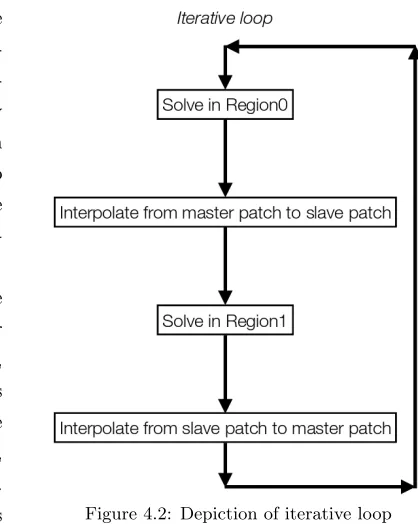
Figure 4.2: Depiction of iterative loop The solver is now created, but it does the same
[image:24.612.284.493.86.351.2]job as it did before, just with a different name and location. The next step is to add interpola-tion between region0 and region1 using patch-ToPatchInterpolation. The description given by OpenFOAM explains that it is an ‘Interpolation class dealing with transfer of data between two primitivePatches’. The thread on CFD Online referenced was a great help, and thanks is re-quired to userbigphil[5].
Figure 4.2 shows the loop necessary for the interpolators to work within the solver. For the regions to be solved one after the other, the solver has to be edited and the regions defined. This next section will describe these steps, in adding the interpolation header files, and adding the files associated with the regions. In the top section of our solver, two lines
should be added, which represent two new files added to the solver. The new section should look like: #include "fvCFD.H" #include "twoPhaseSystem.H" #include "phaseCompressibleTurbulenceModel.H" #include "fixedFluxPressureFvPatchScalarField.H" #include "pimpleControl.H" #include "localEulerDdtScheme.H" #include "fvcSmooth.H"
#include "patchToPatchInterpolation.H" // for patchToPatch #include "regionProperties.H" // for regions/domains
Now that the files are referenced, the solver needs to know what is in them, and they need to be in a place where the solver can find them. patchToPatchInterpolation.H is copied into the model directory, by typing:
cp $WM_PROJECT_DIR/src/OpenFOAM/interpolations/patchToPatchInterpolation /patchToPatchInterpolation.H .
The regionProperties.H file is sourced in the Make/options file. It can be found by doing a ‘find -iname’ in the OpenFOAM main folder, and then referenced accordingly in the options folder. Below the ‘sampling’ line, the following lines should be added,
-I$(LIB_SRC)/OpenFOAM/lnInclude \
4.4. PREPARATION FOR INTERPOLATION CHAPTER 4. START NEW SOLVER
remembering to add the backslash to the above line, and always exclude the backslash from the last line.
The solver can now be recompiled (wclean;wmake) without any errors. If the files were not referenced properly, the compilation would have printed the error. Currently the solver does not solve each region separately; to change this we can use examples from chtMultiRegionSimpleFoam. This solver does what is required here, and so taking lines from its ‘.C’ file, and other ‘.H’ files is a good way to make the hybridModel do the same.
The .C files of the two solvers can be compared, and it should be noticed that in chtMultiRe-gionSimpleFoam.C, there are lines which create fluid and solid meshes (lines 52 and 53). These lines can be added to hybridModel.C, under ‘createMesh.H’:
#include "createFluidMeshes.H" //from chtMultiRegionSimpleFoam #include "createSolidMeshes.H" //from chtMultiRegionSimpleFoam
A distinction needs to be made between each mesh for when it comes to solving them individually later on. These files will now be searched for by the solver, and so should be copied into the hybridModel folder. The two files can be found within the chtMultiRegionSimpleFoam folder, inside fluid/ and solid/. The solver can be found and the files copied over in the usual way. If desired, these file names could be changed to region0 and region1, but since there is only two regions they are left as is in this tutorial. Because of this, the header files do not need editing. It should be also noted that ‘fluid’ and ‘solid’ were defined in section 4.2, in the regionProperties file, and this would need editing if file names were changed.
In the .C file of chtMultiRegionSimpleFoam, it can be seen that inside the runtime loop, there are ‘forAll’ statements for the two regions. This code has to be copied to the hybrid model, and inserted within the PIMPLE loop, for fluid and for solid regions. Belowwhile (pimple.loop()), the forAll statement should be added:
forAll(fluidRegions, i) {
Info<< "\nSolving for first region " << fluidRegions[i].name() << endl;
INSERT PIMPLE LOOP HERE }
along with the Info statement. The PIMPLE loop should be included inside of these brackets, with the same being done for the solid/second region. This will mean that all of of the fluid regions will be solved first, then all of the solid regions. Under ‘createTime.H’, there is another line which references the regionProperties, and this also needs to be added.
regionProperties rp(runTime);
4.5. ADD PATCHTOPATCHINTERPOLATION CHAPTER 4. START NEW SOLVER
4.5
Add patchToPatchInterpolation
The solver is now ready for adding the lines of code required for interpolating. Labels for the master and slave patch need to be created, so that they can be referenced easily in the interpolator code. Below theInfo<< "\nStarting time loop....line, the following two lines should be added:
label master = mesh.boundaryMesh().findPatchID("baffleFace1D_master"); label slave = mesh.boundaryMesh().findPatchID("baffleFace1D_slave");
When ‘master’ or ‘slave’ is used later in the code, this will tell the solver what the definition of the label is.
After the first forAll loop, the first set of interpolators should be added (master to slave patch), and after the second forAll loop, the second set should be added (slave to master). The first include should look like this:
#include "interpolateMasterSlave.H"
Rather than including all the lines of code required in the .C file, the interpolaters are saved as header files in the hybridModel folder, and called with the ‘include’ statement. ‘interpolateMasterSlave.H’ is for master to slave interpolation, and ‘interpolateSlaveMaster.H’ is for slave to master interpolation. The method here shown is to take every variable and pass them on from patch to patch. The file interpolateMasterSlave.H will be described here. The slave to master is of the same format, just with the orders reversed, therefore it will not be explained. At the top of the file, there are some variables listed eg.
volScalarField& k = const_cast<volScalarField&> (mesh.lookupObject<volScalarField>("k.water"));
They are the variables which are not normally editable, and therefore need to be defined and ref-erenced. The listed variables are usually constants, and need overwritten with the const_cast
command. This is not usually recommended in C++, however there are no immediate adverse affects of using it in this case. An example of an interpolator is shown, U1 in this case:
//U1 interpolator note:U1=U.particles (master to slave) patchToPatchInterpolation interpolatorU1
(
mesh.boundaryMesh()[master], // from patch mesh.boundaryMesh()[slave], // to patch intersection::HALF_RAY,
intersection::VECTOR // );
// interpolate from outlet to inlet
vectorField interpolatedInletU1 = interpolatorU1.faceInterpolate <vector>
4.5. ADD PATCHTOPATCHINTERPOLATION CHAPTER 4. START NEW SOLVER
fixedValueFvPatchVectorField::typeName)
FatalError << "inlet patch should be fixedValue!" << exit(FatalError);
U1.boundaryField()[slave] == interpolatedInletU1;
Info<< "inletU1InterpolDomain1 = " << interpolatedInletU1 << endl;
Explaining from the top, the comment states that U1=U.particles, so it is the solid phase dealt with here (U1 is defined in createFields.H). The next line states that patchToPatchInterpolation is used, and the name of this particular interpolator is called ‘interpolatorU1’: this is user defined.
Inside the first set of brackets, we first have the patch to be interpolated from, and then the patch interpolated to, and then definitions of the intersection methods. Master and slave will reference to the lines already defined at the top of the .C file. More information can be found in the intersection.H file, which can be found in the source code, or online on the OpenFOAM C++ Documentation [6]. For direction, there can either beHALF_RAY, which is the normal direction,FULL_RAY, which is both directions, andVISABLEwhich is in the normal direction to the visable part of the surface. Distance is calculated be fitting spheres between the surfaces,CONTACT_SPHEREor by a normal vector,VECTOR. The next section explains that it is a vectorField which is to be interpolated, and that the name of the new variable is ‘interpolatedInletU1’. There then is an error message warning, which prints and causes a fatal error if the patch is not set to ‘fixedValue’. The penultimate line forces the values of the slave patch to become the values of ‘interpolatedInletU1’, meaning the outlet conditions (master patch) become the inlet conditions (slave patch). The final line is an ‘info’ statement that will print to the log file every time the solver passes the line, giving the values of interpolatedInletU1. If tested on the hybrid test case, the log file will print one hundred vector values (x,y,z), which is one for each cell centre: since there are 100 cells in the cross section.
Every other variable should be interpolated like this: U1, U2, P, p_rgh, alpha1, alpha2, K, epsilon, nutWater, nutParticles and thetaParticles. A slave to master file should also be created, ensuring to swap around the patch order, and renaming the variables; an example of U1b is shown below:
//U1b interpolator note:U1=U.particles (slave to master) patchToPatchInterpolation interpolatorU1b
(
mesh.boundaryMesh()[slave], // from patch mesh.boundaryMesh()[master], // to patch intersection::HALF_RAY,
intersection::VECTOR );
// interpolate from outlet to inlet vectorField interpolatedInletU1b = interpolatorU1b.faceInterpolate <vector>
(
U1.boundaryField()[slave] );
4.5. ADD PATCHTOPATCHINTERPOLATION CHAPTER 4. START NEW SOLVER
The files attached to this document can be viewed for more detail if required. The solver can now be tested in the tutorial case. With the following controlDict settings, the solver should run quite quickly, and give similar contour results as if there were no patches present, which means the interpolation is not affecting the results.
controlDict settings:
startTime 0;
endTime 0.04;
deltaT 0.04;
[image:28.612.105.473.149.479.2]writeInterval 0.002;
Figure 4.3: Velocity of water contours: cell values
Chapter 5
Addition of particles to solver
The hybridModel solver now runs smoothly with the interpolation, and so is ready for adding particles. The second phase of the Euler-Euler simulation will be ‘turned off’ as it gets to the baffle, and the Euler-Lagrange will take over, ensuring mass continuity. Adding the parts of DPMFoam and editing the solver to allow for this is explained in this chapter.
5.1
Editing injection method
DPMFoam has several injection methods available: kinematicLookupTableInjection is used in this tutorial, as it allows parameters to be written to a file. The information in the header file of KinematicLookupTableInjection explains what parameters are used and the order they should be in. The following directory contains the different injection models:
OpenFOAM-3.0.x/src/lagrangian/intermediate/submodels/Kinematic/InjectionModel
Below is the description given in the header file of KinematicLookupTableInjection.H.
Description
Particle injection sources read from look-up table. Each row corresponds to an injection site.
(
(x y z) (u v w) d rho mDot // injector 1 (x y z) (u v w) d rho mDot // injector 2 ...
(x y z) (u v w) d rho mDot // injector N );
where:
x, y, z = global cartesian co-ordinates [m]
u, v, w = global cartesian velocity components [m/s] d = diameter [m]
rho = density [kg/m3]
mDot = mass flow rate [kg/m3]
SourceFiles
5.1. EDITING INJECTION METHODCHAPTER 5. ADDITION OF PARTICLES TO SOLVER
The user has a lot of control over the injector, however the lookup table was not designed to be edited as the solver runs. There is therefore no control over how many particles are injected from each location, other than adding more lines to the lookup table. The parameter ‘mDot’ is used to calculate the volume of particles to inject only, and doesn’t actually control the mass flow rate.
The method used here to get around this problem is to define how many particles should be injected from the cell centre location, based on the alpha distribution from the Eulerian phase. This means that there are the same number of rows in the lookup table (one row per cell), and also that a new parameter needs to be created as a new column in the table.
5.1.1
Editing the KinematicLookupTableInjection folder
A new parameter which tells the injector how many parcels to inject from the cell was created, and called numParticles. The following method for editing the source code of OpenFOAM is not the safest, as any errors could follow through into the whole program. Copies of folders to be edited should be made in case this happens. As well as copies of folders, before editing any file in the following sections, a copy of the file was created with ‘org’ at the end of the name; so kinematicParcelInjectionData.H is copied as kinematicParcelInjectionDataOrg.H . A safer way would be to copy over the required code to the user directory, as done with the ‘applications/solvers’ folder.
The first file to be edited is kinematicParcelInjectionData.H. The variable is added as a scalar with name ‘numParticles’, and should be added below the other variables after lines 87, 129 and 150 as follows:
//- No of Particles scalar numParticles_;
//- Return const access to the no of particles inline scalar numParticles() const;
//- Return access to the no of particles inline scalar& numParticles();
These lines entered correctly will create a new data variable, with the last two allowing the new variable to be accessed. The format of these lines are copied from other variables in the header file. kinematicParcelInjectionData.C should be edited to include ‘numParticles’ too, copying the same style as the other variables. After mDot, numParticles should be added with the same format, after the lines 43 and 57:
numParticles_(0.0)
numParticles_(readScalar(dict.lookup("numParticles")))
Note: a comma should be added after mDot in both lists.
5.1. EDITING INJECTION METHODCHAPTER 5. ADDITION OF PARTICLES TO SOLVER
is.check("reading numParticles"); //added by me is >> data.numParticles_;
The following << data.numParticles_ ; should also be added in the list of operators on line 62. This is the file which tells the injector where to look for the variables defined. When numParticles is added at the end of the data list on line 62, the solver will expect to find it in this place.
numParticles should be added in the same manner to kineticParcelInjectionDataI.H. The lines from mDot can be copied an edited, as both variables are scalars. Two sections are added in this file too, after line 57, and after line 92. kinematicLookupTableInjection.H/C should also be edited to suit the new variable. parcelsToInject is already a variable which exists (line 133 of the .C file), and this can be edited to be based upon the new variable ‘numParticles’. The following is the new edited section of parcelsToInject:
template<class CloudType>
Foam::label Foam::KinematicLookupTableInjection<CloudType>::parcelsToInject (
const scalar time0, const scalar time1 )
{
scalar parcelsToInject = 0;
if ((time0 >= 0.0) && (time0 < duration_)) {
// return floor(injectorCells_.size()*(time1 - time0)*parcelsPerSecond_); forAll(injectors_, i)
{
parcelsToInject += injectors_[i].numParticles(); }
Info<< "Time1 = " << time1 << nl << endl; Info<< "Time0 = " << time0 << nl << endl;
Info<< "parcelsToInject = " << parcelsToInject << nl << endl; }
return parcelsToInject;
}
5.2. WRITING LOOKUPTABLE IN SOLVERCHAPTER 5. ADDITION OF PARTICLES TO SOLVER
5.1.2
Editing the InjectionModel folder
No files have changed in this folder, however the solver does not work quite like it should yet. This will be explained in further sections.
After the changes have been made in the two folders, the sections should be cleaned and compiled by navigating back to the src/lagrangian/intermediate folder and typingwclean; wmake.
5.2
Writing lookupTable in solver
Now that the injection method has been changed and a new variable added, the lookupTable code can be added to the solver. This will be written every timestep, and be based on the alpha distribution from the second Euler-Euler phase. Since there will be file writing taking place, and particles being injected, the following two files need to be added to the top list of header files:
#include "OFstream.H" // for writing files etc. #include "basicKinematicCloud.H" // from DPMFoam
As the comments explain, OFstream is for reading/writing files, and the kinematicCloud file is taken from DPMFoam for inserting particles. After adding to the hybridModel.C file, the following lines also need to be added to the Make/options file (not forgetting to add a backslash to the line above):
-I$(LIB_SRC)/lagrangian/basic/lnInclude \
-I$(LIB_USER_SRC)/lagrangian/intermediate/lnInclude \ -I$(LIB_SRC)/lagrangian/distributionModels/lnInclude \ -I$(LIB_SRC)/regionModels/surfaceFilmModels/lnInclude
-llagrangian \
-llagrangianIntermediate \ -llagrangianTurbulence \ -lsolidParticle \
-lsurfaceFilmModels
Cleaning and re-compiling can be carried out after these lines have been added.
The lookupTable should be written after the first region has been solved and after the master to slave interpolation has taken place. This will mean the values written will be the most up to date. Before it is written, there are some new variables which need to be defined and added to the hybridModel.C solver.
5.2. WRITING LOOKUPTABLE IN SOLVERCHAPTER 5. ADDITION OF PARTICLES TO SOLVER
used to get the dot product, by multiplying it by the velocity vector (in C++, the& operator can be used to give the dot product of two vectors).
scalarField dotProduct = U1.boundaryField()[master] & normalSlaveVector;
dotProduct is now divided by the magnitude of the direction vector, to negate the size of the cell.
scalarField uNormal = dotProduct/mag(normalSlaveVector);
Giving uNormal as the velocity vector normal to the surface of the master/slave patch. The final line to be added defines the x,y,z coordinates of the cell centres of the slave patch:
vectorField centres = mesh.C().boundaryField()[slave];
After these lines are added, the lookupTable code can be inserted by using the OFstream appli-cation which allows output to file streams. The first line describes where the file is to be written, in the constant folder in this case, and also the name of the file. The code is inserted below:
const fileName& fName(mesh.time().constant()/"kinematicLookupTableInjection"); OFstream os(fName);
os << "/*---*- C++ -*---* " << endl;
os <<" | ========= | |\n";
os <<" | \\ / F ield | OpenFOAM: The Open Source CFD Toolbox |\n"; os <<" | \\ / O peration | Version: 3.0.x |\n"; os <<" | \\ / A nd | Web: www.OpenFOAM.org |\n"; os <<" | \\/ M anipulation | |\n";
os << "*---*/ //" << endl; os <<"FoamFile\n{\n";
os <<" version 2.0;\n"; os <<" format ascii;\n"; os <<" class dictionary;\n"; os <<" location " "constant" ";\n";
os <<" object kinematicLookupTableInjection;\n}\n";
os <<"// * * * * * * * * * * * * * * * * * * * * * * * * * * * * * * * * * * * * * //\n\n"; os <<"/* (x y z) (u v w) d rho mDot numParcels \n";
os <<" where: \n";
os <<" x, y, z = global cartesian co-ordinates [m] \n";
os <<" u, v, w = global cartesian velocity components [m/s] \n"; os <<" d = diameter [m] \n";
os <<" rho = density [kg/m3] \n";
os <<" mDot = mass flow rate [kg/m3] \n"; os <<" numParcels = number of Parcels \n";
os <<" Dictionary for the KinematicLookupTableInjection */ \n"; os << "( " << endl;
forAll(interpolatedInletU2, i) {
os << centres[i] << " " << U1.boundaryField()[slave][i] << " " << 55e-6 << " " << 2750 << " " << 0.005 << " "
<< floor ((alpha1.boundaryField()[slave][i]*(mag(normalSlaveVector[i]))*uNormal[i])/ ((8.71e-14)*3*(-1)*5000)) << endl;
}
5.3. TURNING OFF INTERPOLATORCHAPTER 5. ADDITION OF PARTICLES TO SOLVER
The first few lines of the file are not really necessary, but are included to make the file look the same as all the other OpenFOAM files. Each line starts with anos <<, and finishes with<< endl;. The characters in-between the quotation marks are the characters that are printed to file.
After all the comments, the important code starts with the forAll statement. This states that for all of the interpolatedInletU2 (the liquid phase) values, do the following. The next line defines what will be printed in each column. Since there are 100 values of interpolatedInletU2 (since there are 100 cells on the plane), there will be 100 rows printed. The data printed in the columns are the same as the line at the top of the comments, each column is explained below.
centres[i] gives cell centre coordinates in (x,y,z) [m]
U1.boundaryField()[slave][i]gives velocity components in (u,v,w) [m/s] 55e-6diameter in [m]
2750 density in [kg/m3] 0.005mass flow rate [kg/m3]
floor ((alpha1.boundaryField()[slave][i]*(mag(normalSlaveVector[i]))*uNormal[i])/ ((8.71e-14)*3*(-1)*5000))gives number of parcels to inject
The last line starts with the wordfloor, which forces the output of the equation to be an integer. This makes sense, as there cannot be ‘half’ of a parcel which contains 3 particles (so 1.5 particles). The equation in written form is: Number of parcels = (alpha of 2nd Eulerian phase * Area of cell * normal velocity component) / (Volume of one particle * number of particles/parcel * number of timesteps/second). This equation is using the volume flowrate to calculate how many parcels should be injected. This could be cleaned up by making the solver search for the variables like diameter etc. in the working directory, rather than the user having to edit the source code everytime they want to make a change to particle parameters. This method was tried, but it was found to be difficult to reference externally whilst inside the ‘forAll’ loop.
Again, the model should be recompiled.
5.3
Turning off interpolator
Now that there is a working lookupTable, the interpolator for the second/solid Eulerian phase can be turned off. If this was not turned off, there would be mass continuity errors in the solver, as there would be double the amount of second phase in region two as there should be; Lagrangian particles and Eulerian 2nd phase.
Inside the ‘solidRegion’ loop, above the Info statement, the following line should be added:
alpha1.boundaryField()[slave] == 0;
5.4. ADDING DPMFOAM CHAPTER 5. ADDITION OF PARTICLES TO SOLVER
Note: commenting large sections can be done quickly by using the following technique:
/* Opens comment
TEXT, TEXT TEXT, TEXT TEXT, TEXT TEXT, TEXT */ Closes comment
The solver will no longer interpolate the alpha or velocity values of the 2nd Eulerian phase from the Master-Slave or vice versa. The solver can be recompiled again.
5.4
Adding DPMFoam
Sections from DPMFoam should now be added to the solver, which will introduce particles. The first piece of code should be added at the very top of ‘solidRegions’ and is as follows:
argList::addOption // from ALopez (
"cloudName", "name",
"specify alternative cloud name. default is 'kinematicCloud'" );
This is taken from Lopez[1], and gives the user the option to specify an alternative cloud name. After interpolating from Slave to Master, but within the loop, add the following:
Info<< "Evolving " << kinematicCloud.name() << endl; // from ALopez kinematicCloud.evolve();
This command will print an info statement, evolve the kinematicCloud, and insert particles as required: more information can be found in Lopez’ tutorial.
This section of code references ‘kinematicCloud’ which needs to be defined in createFields.H. The following lines should be added at the bottom of the file:
Info<< "\nReading transportProperties\n" << endl;
5.4. ADDING DPMFOAM CHAPTER 5. ADDITION OF PARTICLES TO SOLVER IOobject ( "rho", runTime.timeName(), mesh, IOobject::NO_READ, IOobject::AUTO_WRITE ), mesh, rhoInfValue ); dimensionedScalar nu ( transportProperties.lookup("nu") ); volScalarField mu ( IOobject ( "mu", runTime.timeName(), mesh, IOobject::NO_READ, IOobject::AUTO_WRITE ), mesh, nu*rhoInfValue ); word kinematicCloudName("kinematicCloud"); args.optionReadIfPresent("cloudName", kinematicCloudName);
Info<< "Constructing kinematicCloud " << kinematicCloudName << endl; basicKinematicCloud kinematicCloud
(
kinematicCloudName, rhoInf,
U2, // this used to be U1 mu,
g );
This large chunk of code defines the variables, and tells the solver where to find them. It starts off by saying to read the transportProperties file, which contains rhoInf and nu. The bottom gives arguments to kinematicCloud which are the fields to use. Note that U2 is entered here, which means the particle paths are based upon the fluid phase, not the particulate phase.
Chapter 6
Hybrid test case
The model can now be tried out on a test case, to ensure that it is functioning properly. The files that are required are in the attached folder, however some sections will be explained here. The 0 and constant directories are shown below.
0/
alpha.particles alphat.particles alpha.water alphat.water domain0/ domain1/ epsilon.water k.water
lagrangian/ .3 nut.particles nut.water
p prgh
Theta.particles T.particles T.water U.particles U.water constant/
domain0/ domain1/
kinematicCloudProperties kinematicLookupTableInjection particleProperties
phaseProperties regionProperties
thermophysicalProperties.particles thermophysicalProperties.water transportProperties
triSurface/
6.1. RESULTS CHAPTER 6. HYBRID TEST CASE
The directories should look familiar, apart from the domain0 and domain1 sections added. It also must be noted that before the simulation takes place, patches referencing the baffles must also be added. This can be seen by opening 0/p as after the ‘walls’, there are two new entries:
baffleFace1D_master {
type fixedValue; value uniform 1e5; }
baffleFace1D_slave {
type zeroGradient; }
For the users own case, the utility ‘changeDictionary’ can be used. The type should be set to fixed value for the master patches, but the value can be anything, as it will be overwritten by the interpolators. kinematicCloudProperties contains the definition of the injectionModel. The section below is explained with comments.
model1 {
type kinematicLookupTableInjection; //tells solver what type of injection patchName baffleFace1D_slave; //injection patch name
massTotal 3; //this isn't used parcelBasisType fixed; //this isn't used
nParticle 3; //how many particles per parcel - update .C file if changed SOI 0.02; //start of injection
inputFile "kinematicLookupTableInjection"; //input file duration 1; //duration of injection
parcelsPerSecond 50; // doesn't do anything randomise false;
}
kinematicLookupTableInjection will be written as the solver is run, from the OFStream code in the hybridModel.C file. phaseProperties contains the properties of each phase in the Euler Euler simula-tion. regionProperties names each region: fluid and solid in this case. The thermophysicalProperties files contain information about the heat transfer, however this should be negligible as both phases are set to the same temperature. transportProperties defines which phase is the continuous one: water in this case.
6.1
Results
The case should be run with the following commands:
blockMesh
createBaffles -overwrite
6.1. RESULTS CHAPTER 6. HYBRID TEST CASE
As well as the hybrid model, benchmark EE and EL cases were also run. They were set up with the same boundary conditions and parameters as far as possible. The EL injection site was moved to the inlet, as this is a more realistic comparison than injecting from the same location as the hybrid model. Table 6.1 below shows a comparison of the execution times of the 3 models, with two different mass concentrations. As expected the pure EE model is the fastest. The hybrid model is twice as fast as the EL: a marked improvement. If the transition layer was closer to the wall the hybrid model would most likely be faster than this. With the hybrid model taking half the time to solve, this is a promising sign that it is a valid solution to reduce long execution times.
Model Execution Time (s)
1% MC 2% MC
Hybrid model 225 298
Euler-Lagrange 420 585
[image:39.612.180.413.205.267.2]Euler-Euler 102 105
Table 6.1: Comparison of execution times from 0-0.39 seconds with different mass concentrations (MC)
Figure 6.1: Hybrid model showing 2D slice of 2nd Eulerian phase velocity contours, and lagrangian particles in second region also coloured by velocity magnitude.
Figure 6.1 shows a 2D slice though the Z-normal direction of the 2nd Eulerian phase, and also the lagrangian particles coloured by their velocities. The particle injections are based on the values of the 2nd Eulerian phase as explained earlier in the report.
[image:39.612.125.467.316.579.2]6.1. RESULTS CHAPTER 6. HYBRID TEST CASE
6.1. RESULTS CHAPTER 6. HYBRID TEST CASE
[image:41.612.132.463.222.381.2]same scale, so that particle tracks can be directly compared. It can be seen from the particle tracks that there is agreement between the models. To compare in more detail, the particle impacts on the bottom surface are compared in the following two figures. To get this data, the file called ‘PatchPost-Processing.C’ which is a cloud function had to be edited and recompiled. The ‘patchPostProcessing’ section then had to be added under the ‘cloudFunctions’ part of the ‘kinematicCloudProperties’ file, so that the function would be used. This file can be compared to the standard one in the attached files. The data is then outputted in the ‘postProcessing’ folder which is created when a time direc-tory is written. The The z-direction (m) is shown on the vertical axis, and the x-direction (m) on the x-axis.
[image:41.612.135.462.452.614.2]Figure 6.3: EL particle impacts
Figure 6.4: Hybrid model particle impacts
6.1. RESULTS CHAPTER 6. HYBRID TEST CASE
Chapter 7
Conclusions and further work
The hybrid model developed here shows a promising future as a faster way to model slurries, however there are still developments to be made. The volume fraction of the Lagrangian particles in the second region currently has no effect on the first Eulerian phase. This means there is ‘too much’ of the first Eulerian phase in the second region. To rectify this, code from DPMFoam should be added to the hybridModel solver which includes the volume of the particles.
Another issue is the fact that the lookupTable is written every time step but is only read when the solution is initialised. This effectively decouples the solver, and turns it into a steady state problem, since the injection values cannot change so further work needs to be done here.
Chapter 8
Study questions
1. What is the bug in reactingTwoPhaseEulerFoam and what files need to be replaced to solve the problem?
2. What command can be used to create an empty file in a case directory for comparing paraview plots?
3. Name all of the tutorials which use ‘createBafflesDict’.
4. How do you label a patch to your own name for use in the solver?
5. What 3 directions can be used for intersecting in the patchToPatchInterpolation? 6. How can we get the dot product of two vectors in OpenFOAM?
Bibliography
[1] A Lopez. LPT for erosion modeling in OpenFOAM. http://www.tfd.chalmers.se/~hani/
kurser/OS_CFD_2013/AlejandroLopez/LPT_for_erosionModelling_report.pdf, 2014. [2] O Penttinen. A pimpleFoam tutorial for channel flow, with respect to different
LES models. http://www.tfd.chalmers.se/~hani/kurser/OS_CFD_2011/OlofPenttinen/
projectReport.pdf, 2011.
[3] Tobi. All about the PIMPLE algorithm. http://www.cfd-online.com/Forums/blogs/tobi/ 2489-all-about-pimple-algorithm-part-i.html, 2014.
[4] FreeCAD. Freecad. http://www.freecadweb.org/, 2016.
[5] bigphil PatchToPatchInterpolationfaceInterpolate http://www.cfd-online.com/Forums/ openfoam-solving/59868-patchtopatchinterpolationfaceinterpolate.html