A Test setup for characterizing high-temperature thermoelectric modules

Rochester Institute of Technology

RIT Scholar Works

Theses Thesis/Dissertation Collections

7-1-2013

A Test setup for characterizing high-temperature

thermoelectric modules

Satchit Mahajan

Follow this and additional works at:http://scholarworks.rit.edu/theses

This Thesis is brought to you for free and open access by the Thesis/Dissertation Collections at RIT Scholar Works. It has been accepted for inclusion in Theses by an authorized administrator of RIT Scholar Works. For more information, please [email protected].

Recommended Citation

i

A Test Setup for Characterizing

High-Temperature Thermoelectric Modules

by

Satchit B. Mahajan

A Thesis Submitted in Partial Fulfillment of the Requirements for the Degree of

Master of Science in Mechanical Engineering

Approved by:

Dr. Robert J. Stevens

Department of Mechanical Engineering

Dr. Satish G. Kandlikar

Department of Mechanical Engineering

Dr. Michael G. Schrlau

Department of Mechanical Engineering

Dr. Wayne W. Walter

Department of Mechanical Engineering

______________________________ (Thesis Advisor) ______________________________ (Committee Member) ______________________________ (Committee Member) ______________________________ (Department Representative)

Sustainable Energy Systems Lab

Kate Gleason College of Engineering Rochester Institute of Technology

i

Abstract

With the tremendous growth in demand for energy resources, there is a growing need to adopt

alternative energy technologies, including ones that tap renewable energy sources as well as use

non-renewable sources more efficiently. Thermoelectric energy generation is one such emerging

technology. Thermoelectrics can convert waste heat from various sources—significantly, many

industrial processes as well as vehicles—directly into electrical power. Thermoelectric devices

can generate power when a temperature difference is applied across them. Major barriers to

mainstream adoption of thermoelectric devices are their low efficiency and high cost. These are

mostly limited by the properties of the constituent materials of the device(s) and the operating

temperatures. In the past decade there have been significant advancements in thermoelectric

materials that can be used at higher temperatures. The properties of thermoelectric materials are

temperature dependent, and may also vary from bulk material to device level. Right now, devices

with higher working temperatures are not available. According to feedback from laboratories

working on high-temperature modules, the next stage in the development of thermoelectric

devices would go up to 650°C.

The main focus of this project is to design and develop a test stand to evaluate the properties of

all such high-temperature devices. One of the critical challenges in testing modules, especially at

high temperatures, is being able to accurately control and measure heat rates transferred across a

module. Many of the current characterization techniques are limited to solely measuring the

electrical response and ignoring the heat transfer. A new testing technique, “rapid steady state,”

was developed, which is able to accurately measure the three key characteristic properties—the

ii

over temperature ranges from 50 to 650°C. To ensure isothermal surfaces and minimize heat rate

errors, a primary heater is encased in a guard heater. Rapid pulsed electronic loading allows for

rapid voltage-current scans while avoiding thermal drift. The thermal conductivity of a reference

material is used to validate the performance of the guard heater assembly and heat-monitoring

iii

Acknowledgements

First and foremost I offer my sincere gratitude to my adviser Dr. Stevens for his knowledge,

understanding and most importantly patience while guiding me. He had faith in me even at times

when I did not. This project would never have been completed had it not been for his help. I am

not sure how many graduate students are fortunate enough to be given the freedom that you gave

me. For everything you’ve done for me, Dr. Stevens I thank you. I could not have wished for a

better adviser, as a teacher and a person.

I would like to thank NYSP2I for the Research and Development grant which helped fund the

project. I would also like to thank the members of my thesis committee for all their input and

ideas while designing the project. I want to thank Dr. Kandlikar for providing me my first

exposure to experimental testing and Dr. Schrlau for his ideas and insights.

I would like to thank Jan Maneti and especially Rob Kraynik at the Mechanical Engineering

machine shop for their immense help in building the test stand. I would be lost without their

help. I am also thankful to Dr. Hensel and everyone at the ME office for their guidance and

support during my time here at RIT. A special thank you goes to Dhruvang and Reggie, my lab

members for all of their help in completing my project and Sheryl who helped me polish my

thesis.

Finally, I want to thank my family, for always believing in me. They have always been a pillar of

unwavering support and gave me the strength to continue in the face of hardships. I hope that one

day I become at least half the person you thought I would be. I want to also thank my friends

Aditya and Zeeshan, my days in Rochester would be colorless without you. And last I want to

thank my girlfriend Devyani, for being my closest friend, confidant and my silver lining. I cannot

iv

Table of Contents

CHAPTER 1.

INTRODUCTION TO THERMOELECTRICS ... 1

1.1 Introduction ... 1

1.2 Advantages ... 2

1.3 Disadvantages ... 3

1.4 Applications ... 4

1.5 Background and Theory ... 5

1.6 Significant Parameters ... 10

1.7 Thermoelectric Materials ... 11

1.8 TEM Construction and Configuration ... 13

CHAPTER 2.

TESTING APPROACHES ...17

2.1 Harman Approach ... 17

2.2 Steady-State Approach... 20

2.3 Other Testing Approaches ... 24

CHAPTER 3.

PRELIMINARY TESTING ...28

3.1 Steady-State Method ... 29

3.2 Harman Method ... 33

3.3 Gao Min Method ... 48

3.4 Conclusion ... 56

CHAPTER 4.

DESIGN OF THE TEST APPARATUS ...58

v

4.2 Build Overview ... 60

4.3 Thermal Modeling ... 63

4.4 COMSOL and ANSYS Models ... 77

4.5 Build Description ... 84

4.6 Troubleshooting ... 93

4.7 Rapid Steady-State Test ... 98

CHAPTER 5.

VALIDATION AND UNCERTAINTY ...108

5.1 Comparison With the Old Setup ... 108

5.2 Repeatability Testing ... 109

5.3 Validation Using Reference Materials ... 111

5.4 Uncertainty Analysis ... 115

CHAPTER 6.

CONCLUSION ...128

6.1 Summary of Results ... 128

6.2 Contributions to the Thermoelectric Field ... 130

6.3 Suggested Improvements and Future work... 131

CHAPTER 7.

REFERENCES ...134

APPENDIX A ...140

vi

List of Figures

Figure 1.1: Seebeck Effect ... 7

Figure 1.2: Peltier Effect ... 8

Figure 1.3: Variation of ZT with temperature for different materials [11] ... 11

Figure 1.4: Development of ZT since 1940 [13] ... 12

Figure 1.5: Typical thermoelectric module in heat pumping configuration ... 13

Figure 1.6: A typical TEM in power generation configuration ... 13

Figure 2.1: Schematic of the test setup used by Mitrani et al. [27] ... 19

Figure 2.2: Schematic of the test setup developed by Vazquez et al. [30] ... 21

Figure 2.3: Experimental setup developed by Sandoz-Rosado and Stevens [34]... 23

Figure 2.4: Sectional view of the setup used by Ponnambalam et al. [22] ... 25

Figure 3.1: A simplified schematic of the steady-state approach ... 29

Figure 3.2: Module scan for steady-state approach [49]... 31

Figure 3.3: “Heat sunk” test configuration schematic ... 34

Figure 3.4: Current pulse applied to a TEM and the transient voltage generated due to it [50] ... 35

Figure 3.5: Schematic of the experimental setup for the positive and negative tests showing the flow of heat from and into the module... 37

Figure 3.6: Thermal modeling when current is applied in thermal equilibrium [28] ... 38

Figure 3.7: Block Diagram of the experimental setup for Harman method ... 43

Figure 3.8: The plots for voltage and current ... 44

Figure 3.9: The difference of the temperature readings ... 45

Figure 3.10: Thermal resistances in a TEM ... 46

Figure 3.11: Schematic of the Gao Min approach ... 49

vii

Figure 3.13: Schematic for the Gao Min approach ... 55

Figure 4.1: Schematic of the entire setup... 62

Figure 4.2 Schematic of a thermoelectric leg pair ... 65

Figure 4.3: Thermal circuit of the module ... 66

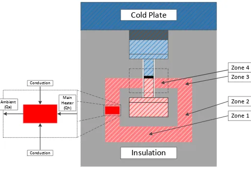
Figure 4.4: Guard heater schematic showing the various zones. Also shown is the discretization method of the guard heater ... 72

Figure 4.5: Thermal circuit for calculating insulation losses ... 73

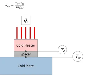
Figure 4.6: Cold side heater assembly ... 76

Figure 4.7: COMSOL simulation temperature distribution ... 82

Figure 4.8: Temperature distribution across the main heater ... 83

Figure 4.9: Temperature distribution across guard heater ... 84

Figure 4.10: Main heater assembly ... 85

Figure 4.11: Sensing thermocouple placement in setup ... 86

Figure 4.12: Control thermocouple placement in setup ... 87

Figure 4.13: Schematic of the argon purging system ... 90

Figure 4.14: Inert gas purging enclosure ... 92

Figure 4.15: Guard heater arrangement with finned base ... 93

Figure 4.16: New design for the guard heater... 94

Figure 4.17: Thermal analysis on redesigned guard heater ... 95

Figure 4.18: Thermocouple calibration setup ... 97

Figure 4.19: Temperature dependence of voltage with an increase in time step ... 100

Figure 4.20: Voltage response for applied current at 10ms time step ... 101

viii

Figure 5.1: Comparison of the characteristic module properties measured by the rapid steady-state approach and the regular steady steady-state approach [34] ... 109

Figure 5.2: Comparison of power output vs. load voltage for different temperature differences ... 110

Figure 5.3: Comparison of voltages and current measurements for different temperature

differences ... 111

Figure 5.4: Comparison of measured conductivity of borofloat and reference values ... 113

ix

List of Tables

Table 2.1: Summary of Literature ... 26

Table 3.1: Steady-State Results for = 150°C and = 50°C... 32

Table 3.2: Comparison of Thermoelectric Module Properties Measured By the Steady-State Approach and Modified Harman approach... 45

Table 3.3: Thermal resistances for a module ... 47

Table 3.4: Comparison With Steady-State Results After Correction ... 48

Table 3.5: Comparison of Gao Min results with Steady state ones, showing the effect of well calibrated resistors ... 56

Table 4.1: The Material Properties Used in Simulation of Extreme CasesTable ... 70

Table 4.2: Properties of Four Extreme Sizes of Thermoelectric Modules ... 70

Table 4.3: Heat Losses Calculated (to the Main Heater and to Surroundings) ... 74

Table 4.4: Cold Plate Heat Flux for Different Temperature Differences ... 77

x

Nomenclature

Symbol Parameter

Surface Area, m2

Current flowing through the leg pair or module, A

Thermal conductance, W/K

* Coverage Factor

Power generated by a leg pair or module, W

Heat rate, W

Electrical resistance of a module, Ω

Thermal Resistance, K/W

Temperature, K or °C

Uncertainty in a measured quantity, %

Voltage across a leg pair or module, V/K

xi

Symbol Parameter

Seebeck coefficient, V

Thompson coefficient, W/mAK

Temperature difference across the module, °C Module efficiency, %

Thermal conductivity, W/mK

Peltier coefficient, W/A

Electrical resistivity, Ωm

xii

Subscript Parameter

Averaged result for tests carried out using positive and negative current

Property measured during negative current test

Property of aluminium block Cold side, K or °C

Cold plate properties Hot side, K or °C

Property evaluated after applying electrical loading

Open circuit

Short circuit

Thermoelectric module

Property measured at ambient condition Properties of thermal bypass

Properties of ceramic plate

Equivalent

Property along insulation

Properties of the interconnect material

Module property

Property of a n-leg

Seebeck component

Property of a p-leg

Overall property over p-leg and n-leg Resistive component

Component of Random uncertainty

Component of Systematic uncertainty

Properties of Shunt resistor

xiii Uncertainty component of voltage

Page | 1

Chapter 1.

Introduction to

Thermoelectrics

1.1

Introduction

In the year 2008, total world requirement for energy was 500 quadrillion BTU [1], approximately

50% of which was dumped into the environment in the form of waste heat. Waste heat is heat

generated in a process by way of fuel combustion or chemical reaction, then “dumped” into the

environment even though it could still be reused for some useful and economic purpose. In the

industrial sector 20–50% of the energy input is lost as waste heat [2].

The energy lost in waste heat cannot be fully recovered because it is often low-grade heat and

dispersed. With the world’s population growing at the rate of 1.1% per year, the energy

requirement is expected to double by 2020 [3]. Coupled with this is the rapid depletion of fossil

fuel global reserves. There is a widespread need for alternative sources of energy and energy

conversion technologies.

The use of thermoelectrics is potentially one such opportunity. Thermoelectric modules (TEMs)

can generate power when placed between a heat source and a heat sink. TEMs are increasingly

finding application in waste heat regeneration such as automobiles, industrial processes, and

power plants. This is a process wherein heat energy that would have been dissipated into the

atmosphere is utilized for generating power. Thermoelectrics are also environmentally friendly

Page | 2

Another important application of thermoelectrics is as Peltier coolers. These are extensively used

in electronic devices that have specified cooling requirements. Precise temperature control and

the abbility to cool below atmospheric temperatures make them an ideal candidate in computer

electronics.

1.2

Advantages

There are many advantages to using thermoelectrics. These are summarized as follows:

No moving parts: Thermoelectrics can generate electricity directly without any moving parts so

they are virtually maintenance free. In fact, one of the first applications of thermoelectrics was

and still is to power deep space probes using radioisotopes as heat sources. These systems have

functioned for decades with no maintenance [4].

Small size and weight: The overall thermoelectric cooling system is much smaller and lighter

than a comparable mechanical system. In addition, a variety of standard and special sizes and

configurations is available to meet strict application requirements. Thermoelectrics are modular

and can be used for a range of applications. Current systems operate over a wide range, from

mW to KW.

High reliability: Thermoelectrics exhibit very high reliability due to their solid state

construction. Although reliability is somewhat application dependent, the life of typical

thermoelectric coolers is rated to be greater than 200,000 hours. The actual life of the modules

may be much longer. In fact, the modules used by NASA in their long-range satellites are still

Page | 3

Operational conditions: Thermoelectrics can be used in any orientation and adverse

environments, as well as over a large range of temperatures. This makes them ideal for

applications based on waste heat utilization.

Transient heat sources: TEMs can be used in applications where the heat source is not constant.

This is a huge benefit in applications like waste heat utilization of automobile exhaust, where the

heat source is variable and where other power recovery technologies are not feasible.

1.3

Disadvantages

Though thermoelectrics have many advantages, there are drawbacks in the technology. These are

summarized as:

Low efficiency: This is a major drawback facing the thermoelectric industry. Current

off-the-shelf thermoelectric devices efficiencies are typically in the range of 2–8%. Thermoelectrics

have been mainly confined to low-energy applications or where the heat source is free, and are

unable to compete for large-scale power generation applications.

Susceptibility to shock loading: Thermoelectrics can handle transient heat loads, but the life of

thermoelectric devices decreases considerably after receiving thermal shock loading. In the case

of mechanical loading, they can withstand up to 1000 psi but only to the standard loading—

around 200psi—in compression. They are weakest in shear loading [5].

Cost: Owing to the novelty of the technology, the cost per watt of the device is much higher than

with the conventional power generation technologies. As newer and cheaper materials with

higher power ratings are developed and manufacturing techniques are improved, the cost per unit

Page | 4

1.4

Applications

Peltier cooling

Peltier cooler is a thermoelectric operating in heat pumping mode. As current is passed through a

thermoelectric device, a temperature difference develops across it. The cold side of the device is

thermally coupled with the component being cooled, while the hot side of the device needs to be

cooled externally using a heat sink or forced convection. Peltier coolers have an important role in

electronics, especially in cases where conventional cooling systems cannot be implemented.

Their small size, silent operation, and the ability to maintain the temperature accurately make

them especially attractive for use as CPU coolers [6].

Thermoelectrics are also used in microelectronics where localized cooling is required. Gupta et

al. [7] investigated the operation of a ultrathin thermoelectric cooler for cooling of localized hot

spots on a chip. They found the device to be very effective for low-current operations. However,

as the current increased over 4A, back heat flow due to the temperature difference generated

countered the cooling effect.

Other niche applications include refrigeration, in wine coolers, car refrigerators, and beverage

can coolers. Thermoelectrics are also used in NEMA enclosures to regulate temperatures and

applications where cryogenic cooling is required.

Power generation

While thermoelectrics are not currently used in a wide range of power generation applications,

their most important application will undoubtedly be in power generation. An important factor is

Page | 5

energy conversion efficiency is low compared to other power conversion technologies, which is

the main hurdle to be crossed before thermoelectric moves from a niche to mainstream power

generation applications.

Low-power applications include powering watches, calculators, and remote sensing. The

“Thermic” [8] designed by Seiko used body heat for its working. Thin film micro generators

producing power at milliwatt and microwatt level are used in electronic applications. Kim [9]

fabricated one such device generating 4.3nW/K. These can be coupled easily with photovoltaic

cells as well.

Thermoelectrics have found application in high-power generation as well, but the major

drawback is the low efficiency. They are mainly used in waste heat applications, where the

supply of heat is free. Commercially, modules generating up to 550W are available. Standalone

thermoelectric generators are mainly used in extreme environments.

Thermoelectrics have been critical in enabling continuous powering of deep space probes where

the use of solar and other power generation technologies is not feasible. For example,

thermoelectrics are used in radioisotope thermoelectric generator (RTG) where power is

generated using heat from the decay of radioactive material, like plutonium-238. Over the last

four decades, 26 missions have used RTGs. The RTG installed on the Mars rover is expected to

operate for at least one Mars year or 687 Earth-days.

1.5

Background and Theory

Thermoelectric devices are basically solid state devices that can convert energy from heat to

Page | 6

common being bismuth telluride. A typical configuration of a thermoelectric module consists of

many leg pairs made of semiconductor pellets, joined together using contact tabs made of high

conductivity materials.

Seebeck Effect

The principle behind the working of the thermoelectric module is the Seebeck effect. In 1821

Thomas Johann Seebeck observed that when two dissimilar metals with junctions at different

temperatures are connected in a circuit, a magnetic needle would be deflected. Seebeck initially

attributed this phenomenon to magnetism. However, it was quickly realized that it was an

induced electrical current that deflects the magnet [10]. In a thermoelectric module, the two

dissimilar conductors are connected electrically in series and thermally in parallel. When the two

Page | 7 Heat In

Heat Out

Hot Junction (TH)

Current

Power Generation

Cold Junction (TC)

Figure 1.1: Seebeck Effect

The voltage produced is proportional to the temperature difference between the two junctions.

This is given by:

(1.1)

The proportionality constant, α, is the difference between the Seebeck coefficients of the two materials forming the junction. This is known as the overall Seebeck coefficient, and often

referred to as the thermoelectric power or thermo power. The Seebeck voltage does not depend

on the distribution of temperatures along the material between the junctions. This phenomenon is

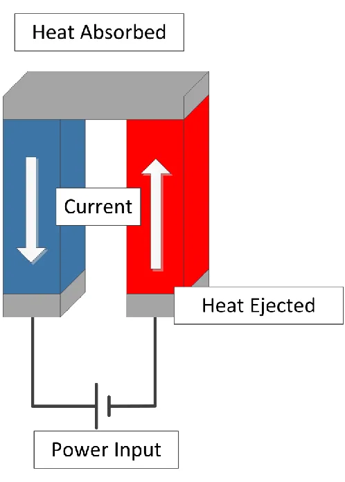
Page | 8 Peltier Effect

The converse of the Seebeck effect was discovered independently by Jean-Charles Peltier in

1834. When current is made to flow through a junction of dissimilar materials, a rate of heating

occurs at one junction while heat is absorbed at the other junction [10]. Although it is the

converse of the Seebeck effect, Peltier failed to make the connection when he discovered the

phenomenon. In Fig. 1.2 it can be seen that when a current is passed through the junction, one

side is heated and the other is cooled.

Figure 1.2: Peltier Effect

The Peltier co-efficient is defined as:

Page | 9

where Q is the rate of heating or cooling and I is current passing through the junction. The Peltier coefficients represent how much heat current is carried per unit charge through a given material

[10].

Thomson effect

The Thomson effect was observed by Sir William Thomson in 1851. It relates to the rate of

heating or cooling resulting from the passage of current through a current-carrying conductor

with a temperature gradient applied across it, and is defined as the evolution or absorption of

heat when electric current passes through a circuit composed of a single material that has a

temperature difference along its length. If ( ) is the temperature difference generated across a

conductor carrying current ( ), then heat generated per unit length ( ̅) is given by

̅ (1.3)

where is the Thomson coefficient.

The Kelvin Relationships

Lord Kelvin developed relationships between the above three thermoelectric coefficients. The

relationships were tested for many thermoelectric materials and it is assumed that they hold true

for all materials used in thermoelectric applications.

The relationships can be written as:

(1.4)

(1.5)

Page | 10

1.6

Significant Parameters

The most important parameters in a thermoelectric material are the “Seebeck coefficient” and

“figure of merit.” The Seebeck coefficient is a measure of the transported entropy per charge

carrier. The figure of merit is a non-dimensional measure of performance of the material. It gives

the theoretically possible maximum efficiency of a thermoelectric.

The figure of merit (ZT) is expressed as

(1.6)

The figure of merit varies directly with the Seebeck coefficient and electrical conductivity and

inversely with thermal conductivity. An increase in electrical conductivity reduces the losses

caused due to Joule heating. A decrease in the thermal conductivity would limit the amount of

heat passing through the module without being converted into power. The theoretical maximum

efficiency of thermoelectric material depends on the figure of merit, and there are no theoretical

upper limits for the figure of merit. Most materials currently used have thermoelectrics of

approximately one or less. Figure 1.3 shows the relationship between the TZ values of different

Page | 11

Figure 1.3: Variation of ZT with temperature for different materials [11]

Though the ZT value is the measure of a Carnot performance, it does not exactly translate to the module efficiency. The efficiency actually is based on the amount of heat flowing through the

module itself, not the amount of heat available. A clear trend is observed, where ZT for a given

material increases as its temperature increases. Currently, the best thermoelectric materials

developed in the lab have values between one and three[11], but these are yet to be used in

practical devices.

1.7

Thermoelectric Materials

Low efficiency of the thermoelectric modules is a significant drawback hindering the use of

Page | 12

begets better efficiency. Hence, extensive research is being carried out to find a material with

high ZT and to improve the ZT values of existing materials.

In the literature today, the best materials currently used in most thermoelectric devices have ZT

values between zero and three. Some of the most popular materials have been bismuth telluride

(Bi2 Te3 system) and silicon-germanium combinations. Much research has been carried out on

these materials and the scope of improvement is small. Consequently, newer and better materials

are being investigated, primarily by nano-engineering materials. Figure 1.4 below shows a plot

of ZT as a function of temperature for the various nanostructured bulk materials being developed

in labs. There have been tremendous improvements in thermoelectric materials, primarily driven

by improved understanding of thermal transport at the nanoscale and improved nanostructure

fabrication techniques [12].

Page | 13

1.8

TEM Construction and Configuration

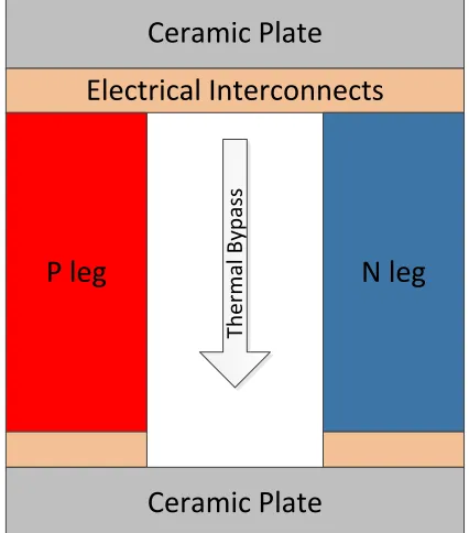
A typical thermoelectric module is made of multiple leg pairs, where each leg pair is made of

two semiconductor materials made from p and n type semiconductor materials. The combination

of these multiple leg pairs is held together by a top and bottom plate, typically made of a

ceramic-like aluminum nitride (AIN). This ensures electrical insulation and structural support.

The leg pairs are connected in such a way that they are in series electrically and in parallel

thermally. The pellets, tabs, and ceramic plates form a layered configuration, as seen in Fig 1.5.

Figure 1.5: Typical thermoelectric module in heat pumping configuration

Generally the individual legs are made of a single material. But as newer technologies are

developed, leg pairs made up of multiple materials are being developed.

Page | 14

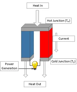
Figure 1.6 shows a module in a power generation arrangement where heat enters the hot side of

the module and is rejected from the cold side of the module. The most commonly used approach

for calculating power generation is a one-dimensional approach. Using the model developed by

Angrist [14] , the heat flow into the hot side of the module, , is expressed as

⁄ (1.7)

where I is the current flowing through the module and is the overall Seebeck coefficient, which is the product of the difference of the individual Seebeck coefficients of the two

constituent materials and the number of leg pairs. and are the temperatures on the hot and

cold sides of the module. K is the thermal conductance, which is the inverse of the thermal resistance across the entire device. This includes the thermal resistance of the legs as well as the

thermal resistance of the substrate and thermal leakage across the device. R is the electrical resistance, which includes the leg and metal connector contact resistance. The heat flow out of

the module ( ) is given by

⁄ (1.8)

These expressions are developed by solving the heat diffusion equation in the device and

applying a fixed temperature and the Peltier effect model at the surfaces. From energy

conservation, the electrical power output of a thermoelectric module is expressed as

(1.9)

Page | 15

The efficiency of the module can be expressed as the ratio of the power output to the heat input,

and is given as

(1.11)

⁄

Most of the modules commercially available today can be classified as “low temperature.”

Research conducted on low-temperature waste heat recovery systems [15–19] has demonstrated

the potential viability of thermoelectric systems. However, the primary reasons that

thermoelectrics have not been adopted in mainstream applications are low efficiency and high

cost. The efficiency of the module generally increases as the temperature difference applied

across it increases. To achieve improved efficiency, there is interest in developing

high-temperature materials to enable operation of modules at higher high-temperature differences than

those reached with typical BiTe-based devices.

In conclusion, over the past decade there have been significant advancements in thermoelectric

materials that can be used at high temperatures [20–24]. More recently, TEMs based on these

materials have also been developed. Thus, developing the capability to test high-temperature

thermoelectric devices is desperately needed to support the development of ceramic oxide-based

thermoelectrics. Such capabilities do not currently exist. The testing system proposed in this

thesis will provide the ability to demonstrate proof of concept of the next generation of

thermoelectric devices using oxides and other high-temperature materials, provide experimental

Page | 16

purposes. The testing capabilities will also allow for an efficient means of optimizing devices

Page | 17

Chapter 2.

Testing Approaches

In the field of thermoelectrics, there are two categories of testing. The first is testing of materials,

and the second is testing of modules or devices. A wealth of research on the testing and

characterization of thermoelectric materials exists. However, little has been done to test complete

power generation modules. Material testing cannot account for different performance effects

such as diffusion losses, contact resistance, thermal strain, and thermal cycling that occur in

power generation modules. Module level testing is also vital for quantifying device performance,

validating existing models, and optimizing module design, as well as testing for longevity and

reliability of a device.

There have been two main approaches used for characterizing modules in the literature: the

Harman approach and the steady-state approach. Both approaches have been utilized for low-

and high-temperature testing in literature. This chapter describes some of the setups and analysis

used for testing modules as well as bulk materials.

2.1

Harman Approach

The Harman approach [25] was initially developed for bulk material testing, but has been

adopted and used for module testing. The technique is based on the Peltier effect of a

thermoelectric material, specifically the heating and cooling at the module interfaces when a

current is applied. When a current is passed through a module, the voltage across the module

Page | 18

asymptotically increases to the steady-state voltage, which is the sum of the resistive and

Seebeck voltage. The Seebeck voltage is caused by the temperature difference developed in the

device due to the Peltier cooling. The voltage is given by Eq. (1.1). When the current is removed

from the module, the voltage drops instantaneously to the Seebeck component of the voltage and

then decays to zero as heat conducts across the module and returns to being isothermal. The

various properties are calculated using these voltages and resulting temperatures, and is

described in detail in Section (3.2).

The method initially developed by Harman [25] uses the difference between the total voltage and

the electrical resistance component of the voltage to calculate the Seebeck coefficient for the

module. The method does not take into account effects like Thomson heating and joule heating,

and heat losses due to conduction are assumed to be negligible. The method was validated by

comparing values of properties with a reference material. A variation of this method was

developed by Buist [26]. It uses the Seebeck component of voltage measured; specifically, the

voltage immediately after the applied current is removed, to calculate the Seebeck coefficient.

The approach called for bipolar testing to reduce errors and maximize accuracy of the results.

This is explained in detail in Section (4.2). The method also includes a correction factor for the

various heat losses.

Mitrani et al. [27] successfully used Buist’s method to calculate module performance parameters.

Instead of performing an energy balance, they used a reference material (aluminum) to calculate

the thermal conductance of the module. The results were found to match the ones from

steady-state testing as well as from electrothermal modeling in SPICE. A drawback of this general set of

approaches is that it is difficult to measure thermoelectric properties above room temperature.

Page | 19

the ambient, which makes it difficult to maintain adiabatic conditions on the module. Figure 2.1

shows the schematic of the test setup used.

Figure 2.1: Schematic of the test setup used by Mitrani et al. [27]

Fujimoto et al. [28] attempted to overcome the issues with high-temperature testing by reducing

thermal heat flow from the environment with a thermal anchor and a thermal reflector. They also

accounted for heat losses from wire conduction and ambient radiation. An important discovery

made while testing was that the largest cause of contact resistance was improper soldering at

contacts. They applied corrections to better account for the effect of contact resistance, and

reduced it by using a particular soldering technique.

The Harman approach can overlook convection losses by using a low vacuum. In cases where a

vacuum is not used, a correction factor was developed by Lau [29] to account for convection

effects. The correction factor was obtained by testing a module in both air and a vacuum and

comparing the results. However, even with the correction factor, it was observed that some

Page | 20

materials with good, repeatable results, most of the testing is performed at room temperature.

Consequently, one of the downsides is that modules are not tested under typical operating

conditions.

2.2

Steady-State Approach

The second approach, the steady-state approach, ensures modules are tested under more realistic

operating conditions. The testing approach is for a steady setup is relatively straightforward and

the most common approach for module testing. One of the surfaces of the module is maintained

at a high temperature while the other is maintained at a lower temperature. According to the laws

of thermoelectricity, specifically the Seebeck effect, a potential difference is developed across

the module. By measuring the heat flows into or out of the module along with the voltage and

current, the module parameters can be estimated. An important assumption for the steady-state

approach is that all heat losses are measurable and accounted for. Measuring the exact amount of

heat rate flowing into or from the module is of utmost importance. However, obtaining an

accurate measurement is often challenging. As this is such an important part of the approach, the

various test stands in literature have been classified based on how they account for heat losses.

They are classified as basic setups, where the heat losses are considered negligible because the

setup is insulated well; passive accounting, where the heat losses are accurately measured and

accounted for; and active accounting, where the heat losses are measured as well as minimized

by using special guards.

Basic setups

Vazquez et al. [30] describe one such test stand for temperatures up to 300°C. The temperature

Page | 21

one varied the hot side temperature and the second varied the hot side heat flux. The cold side

was kept at a constant temperature. The various properties were calculated by loading the

module with various resistors and plotting the relationship of the voltage versus the current. One

drawback of the setup is that it does not account for any heat losses. The schematic of the setup

is shown in Fig. 2.2.

Figure 2.2: Schematic of the test setup developed by Vazquez et al. [30]

Tanji et al. [31] developed a steady-state test setup for testing of modules developed by a new

type of assembly method. The setup observes the importance of applied pressure on the module

and the effect of contact resistance. To reduce the contact resistance, they used a metallic paste

of liquid InGa and solid Zn.

Another setup was developed by Hsu et al. [32] for modules up to 250°C. Although they did not

account for heat losses, they provided a good explanation for the difference between material and

module properties. They also observed the effect of loading pressure on the measured module

parameters. Furthermore, an important method of relating the measured and theoretical

properties was developed. The properties discussed in the previous literature were material

Page | 22

experimental results. The main reason for the discrepancy was the effect of the temperature

gradient across the components of the module. This gradient was accounted for by using thermal

resistances across each component to determine the actual temperature gradient across the

thermoelectric module.

Passive accounting

Anatychuk and Havrylyuk [33] developed a test stand for measuring parameters up to 600°C that

accounts for heat losses from the hot side to the surrounding environment. The test stand uses a

heat meter attached to the cold side heat exchanger, which measures the heat flux flowing out of

the module. The heat meter used was a reference material of known conductivity such that the

exact heat rate could be calculated using the temperature difference measurement. At

steady-state conditions, it was assumed that the amount of heat flowing in will be equal to the amount of

heat flowing out of the module. In order to accommodate different-sized modules, the setup

employed interchangeable heat meters with an area resembling the module being tested. To

minimize errors, the hot side was well calibrated using a protective heater. The authors also

calculated the uncertainty in measurement, which was found to be 3%.

Another test stand was created by Sandoz-Rosado and Stevens [34] to characterize modules up to

500°C. The heat losses through the insulation on the top and sides of the heater as well as

through the insulation surrounding the sides of the module were measured. A power analyzer

measured the power input to the heaters. The authors also accounted for the effect of contact

resistance by loading the module with different pressures to measure its performance. Figure 2.3

Page | 23

Figure 2.3: Experimental setup developed by Sandoz-Rosado and Stevens [34]

Muto et al. [35] developed a setup used to measure properties of bulk materials for temperatures

up to 200°C with low uncertainty. These measurements also included the effects of side wall

radiation and contact resistance. The researchers encountered large heat losses from the hot side

assembly. To overcome this issue, they used a well-calibrated flux sensor on the cold side to

measure the heat flux, which accounted for heat losses by calibrating the flux sensors. The

authors used both approaches of the passive accounting—calculating heat losses and using a heat

meter—to verify their calculations.

Although these techniques are used extensively at lower temperatures, calculating heat losses at

higher temperatures leads to large uncertainties in measurements. The use of a reference material

also has certain drawbacks, the most important being the accuracy of data available for the

Page | 24

measuring accurate temperature gradients within the reference material as well as calculating

heat losses from the reference material.

Active accounting

To overcome the inherent errors in using passive accounting techniques, researchers have used

radiation shields and shielding heaters to minimize heat losses. Rauscher et al. [36,37] use a

shielding heater to minimize heat losses. The principle behind this approach is that any heat loss

is related to a temperature difference in the system. If this difference is minimized, the losses can

be minimized. A shielding heater is basically an outer heater that surrounds the heater in contact

with the thermoelectric module. This ensures that all the heat supplied to the main heater block

passes through the module and not to the surroundings. A similar approach was used by

Takazawa et al. [38] in their setup to test modules up to 550K. They utilized a radiation shield to

reduce heat losses at the upper temperature limits.

2.3

Other Testing Approaches

Apart from the two main approaches described above, researchers have also experimented with

other methodologies to measure thermoelectric module parameters. Min and Rowe [39–41]

developed a testing method based on the steady state but eliminating the need to measure the

heat fluxes. This novel method utilizes an open-circuit and short circuit measurement to calculate

module parameters. Even though it is steady state, it does not require the measurement of the

exact amount of heat flowing through the module. This makes it especially attractive at high

temperatures, where this measurement is difficult by traditional means. To investigate its

application at high temperature, a detailed analysis was performed which is described in Section

Page | 25

Similar to the Harman method, a transient method was developed by Middleton and Scanlon

[42]. They used the method to measure the thermoelectric properties of germanium from 78–

925K. The Seebeck coefficient was calculated using the change in voltage brought about by the

change in temperature. To calculate the electrical resistance, the voltage response on the passage

of current was used. This approach is known as the differential approach and was developed

specifically for bulk materials. Sharath Chandra et al. [43] and Paul [44] developed high

accuracy setups based on this approach. The setup developed by Ponnambalam et al. [22] is

shown in Fig. 2.4.

Figure 2.4: Sectional view of the setup used by Ponnambalam et al. [22]

Table 2.1 shows a brief summary of the different testing methods reported in the literature along

Page | 26

Table 2.1: Summary of Literature

Author Approach Temp. Range Material Vacuum

Harman, T. C. [25]

Harman 300K Bismuth telluride Low vacuum

Buist and Richard [26]

Harman <330K N-type bismuth

telluride

—

Mitrani et al. [27]

Harman 300K Module —

Fujimoto et al.

[28]

Harman <600K N-type bismuth

telluride

Low vacuum

Lau [29] Harman 300K Module Low vacuum, air

Vazquez et al.

[30]

Steady state <573K Module —

Tanji et al. [31] Steady state <573K Module —

Hsu et al. [32] Steady state <523K Module —

Anatychuk and

Havrylyuk [33]

Steady state <873K Module —

Sandoz-Rosado

and Stevens [34]

Steady state <773K Module —

Muto et al. [35] Steady state <473K P-type bismuth telluride

_Torr

Rauscher et al.

[36]

Steady state <573K Module Low vacuum

Rauscher et al.

[37]

Steady state <573K Module Torr

Takazawa et al.

[38]

Steady state <550K Module Torr

Ahiska and

Ahiska [45]

Page | 27

Author Approach Temp. Range Material Vacuum

Ciylan and

Yilmaz [46]

Steady state <373K Module —

Min and Rowe

[39–41]

Steady-state

based

<373K Module —

Iwasaki et al.

[47]

Harman based <315K Module Torr

Middleton and

Scanlon [42]

Differential 78–925K Germanium High vacuum

Paul [44] Differential 100–600K P-type PbTe 5 Torr

Sharath Chandra

et al. [43]

Differential 300K Al doped FeSi

platinum

_Torr

From the literature review, it is clear that gaps exist in the area of high-temperature testing of

modules. The main reason for this is modules that can be tested at high temperatures have yet to

be developed. The high temperature setups developed are also found to yield fairly inconsistent

results because of a lack of standardized guidelines for the measurement procedure [22,48]. This

makes the selection of testing approach very difficult.

In summary, the popular choice for module testing seems to be the steady-state approach, but

high temperature testing will encumber active accounting of heat losses. The Harman approach,

though not extensively used for module testing at high temperatures, was the most used for

testing of material properties. The Gao Min approach is also a possible choice as it does not

Page | 28

Chapter 3.

Preliminary Testing

Preliminary testing is important gauging response time of the setup, determine ability to maintain

operating conditions and determine accuracy of instrumentation required. Of the various

approaches discussed in the literature for measuring module parameters, three were narrowed

down as candidates for the proposed high-temperature testing system. To determine the best

overall testing system, three preliminary setups based on the principles of the steady-state [34]

approach, Harman[26]approach, and the Gao Min [39] approach were developed to better

understand the various issues associated with each method before designing the high-temperature

test setup, the primary goal of this research.

The results from the three setups were compared for modules at low temperatures. Information

about module parameters is readily available for low temperatures, making comparison easy. A

commercially available BiTe module (Thermonamic Electronics TEP1-1264-1.5) with 126 leg

pairs was used. The size of the module was 40mm x 40mm, with 50% fill area, meaning 50% of

the module was air. Tests were conducted at a constant loading pressure and with thermal grease

on both sides of the module. Considering the rudimentary design, an uncertainty of 10% was

assumed. All the tests were performed at an average temperature of 100°C to keep the results

comparable. Multiple tests were performed on the same module to ensure repeatability in

measurements. All measurements were made using the same DAQ devices: NI–USB 6008 for

Page | 29

3.1

Steady-State Method

The test setup developed by Sandoz-Rosado and Stevens [34] was successful as a tool for

characterization of module performance. The major achievement in the setup was to quantify the

heat transfer to the hot side of the module while adjusting the temperature difference across

devices under a wide range of electrical loads. Using measurements of the current, voltage, and

the hot side and cold side temperatures, the Seebeck level of the device, electrical resistance, and

thermal conductance parameters can be determined. Tests were carried out at various loading

pressures and temperatures, and a platform for characterizing module performance was

developed. Working with this test setup provided an insight into the various problems that may

arise, albeit only for low temperatures. A simplified schematic of the steady-state approach can

be seen in Fig. 3.1.

Page | 30

The size of the module to be tested was much smaller than the size of the heater. The model

developed by Rosado-Sandoz and Stevens [34] was used in calculating the heat loss from the

heater.

A typical test involves a device subjected to a fixed temperature difference and held until

temperatures and the heat flux have stabilized, which typically takes nearly an hour to reach a

steady state. Once a steady state is reached, a scan at different electrical loads is performed.

Although one could extract the electrical resistance and fully characterize the device using only a

short-circuit current and open-circuit voltage measurement, a scan over many operating points

along the voltage-current curve will improve confidence in the device’s parameter calculations.

For a scan, the module is connected to an automated electrical loading box and 12 different loads

are automatically applied to try to sweep the entire current-voltage curve for the device. Between

each of the 12 steps, the module is allowed to reach a steady state. The time for these varies

because heat rates change as a function of the operating current, as can be seen in Equations (1.7)

and (1.8). This scan of voltage-current data provides the basis for calculation of thermoelectric

performance parameters of a device. The scan obtained from the test setup is exported into Excel

for further analysis. The properties are calculated by two different means and then compared.

The three required module parameters are the device-level Seebeck coefficient, electrical

resistance, and thermal resistance.

The principal approach to extracting module parameters is to minimize the residuals between the

measured values of voltages and hot side heat rates and their theoretical values by varying the

Page | 31

Figure 3.2: Module scan for steady-state approach [49]

The theoretical heat rate is given by Eqn. (1.7) and the theoretical voltage can be obtained by

dividing the power Equation (1.10) by the current to give the voltage as:

(3.1)

Residuals are measured as the square of the difference between the two values to account for

positive and negative errors. The minimization provides one set of the values of the module’s

parameters, the slope, and the y-intercept of the current-voltage line.

The y intercept gives the open-circuit voltage ( ) and the slope of the plot is equivalent to the

electrical resistance ( ). The Seebeck coefficient ( ) is calculated as:

Page | 32

The thermal conductance of the module can be expressed as the ratio of the actual heat to the hot

side of the module under open-circuit conditions to the temperature difference across the

module:

(3.3)

The module effective figure of merit, ZT, is calculated as:

(3.4)

The values obtained from Eqns. (3.2) - (3.4), and the slope of the line ( ), are compared with the

values from the minimization scheme. The two sets of values are found to be in agreement with a

difference of less than 5%.

The tests were carried out multiple times to test for repeatability. The results, averaged over

multiple tests, were tabulated as seen in Table 3.1.

Table 3.1: Steady-State Results for = 150°C and = 50°C

Properties Steady State (397K)

α (V/K) 0.044

R (Ω) 2.42

K (W/K) 0.63

ZT 0.47

As mentioned earlier, as this setup is the most developed one, it will be used for low-temperature

Page | 33

3.2

Harman Method

To obtain accurate results, the steady-state approach requires careful estimation of all possible

heat losses, which becomes challenging at high temperatures. The experimental time is also

significant. An alternative to the steady-state setup is the Harman approach. The key to this

method is a computer-driven, high speed, high resolution, integrating voltage measurement

system capable of accurately resolving the voltage components in an active thermoelectric device

or sample [26]. In order to determine the effectiveness of this approach, a prototype of such a

setup was built and a model tested at low temperatures as a proof of concept.

This approach has many advantages over the steady state. It provides for the measurement of all

the parameters needed to characterize the thermoelectric properties of a module. The current

requirement for Harman approach is very low. For low-temperature applications, it was observed

that the transient setup requires a current 1/50th of that required for the steady-state setup [50,51].

Another advantage is that it can be used to potentially determine the cause of the failure of a

device.

To accurately test properties of a module, the arrangement used was the “heat sunk”

configuration. This involves maintaining adiabatic conditions on the cold side to control the

temperature, as seen in Fig. 3.3. Advantages of this configuration include potentially quicker

testing and simplicity of the connections. There were four quantities that need to be measured to

characterize a thermoelectric device: the Seebeck voltage ( ), the steady-state current ( ) under

Page | 34

Figure 3.3: “Heat sunk” test configuration schematic

When a current is applied to a thermoelectric device, a voltage develops across it. This voltage is

a combination of the resistive voltage ( ) and the Seebeck voltage ( ). The applied current also

generates a small temperature difference across the module ( ).

The total potential difference across the module can be written as:

(3.5)

where

(3.6)

(3.7)

The Seebeck coefficient and electrical resistance are calculated as

(3.8)

(3.9)

where is the applied current. The thermal conductance ( ) is calculated using the energy

Page | 35

The test to determine the module properties is based on the measurement of . When a current

is applied to an isothermal module, the voltage rises instantaneously to value and then

asymptotically increases to , as a temperature difference develops across the device because of

the Peltier cooling and heating at the two interfaces. When the current is turned off, the voltage

instantaneously drops to and then decays to zero as the module become isothermal over time

due to conduction [50]. The measurement of the value is the basis of the modified Harman approach. Figure 3.4 shows the nature of the current applied and its corresponding output

voltage. The figure uses S as an abbreviation for the Seebeck coefficient, whereas the symbol used henceforth is α.

Figure 3.4: Current pulse applied to a TEM and the transient voltage generated due to it [50]

The tests conducted are bipolar processes. The test is carried out using one polarity of the

current; the current is then reversed and the test repeated [50]. Bipolar testing is essential as it

Page | 36

associated with Joule heating, and wire losses, and to reduce the magnitude of a correction

factor. In the modified Harman method, it is assumed that the thermocouples used are perfectly

identical. If this is not the case, additional errors may be encountered. Bipolar testing process

corrects for any imperfections caused by non-identical thermocouples.

Derivation for the heat sunk case

The calculation of the Seebeck coefficient () and the electrical resistance (R) is straightforward. To calculate thermal conductance (K), the model developed by Buist [50] was used by modifying it to suit the heat sunk case. The figure of merit can be calculated with the help of the standard

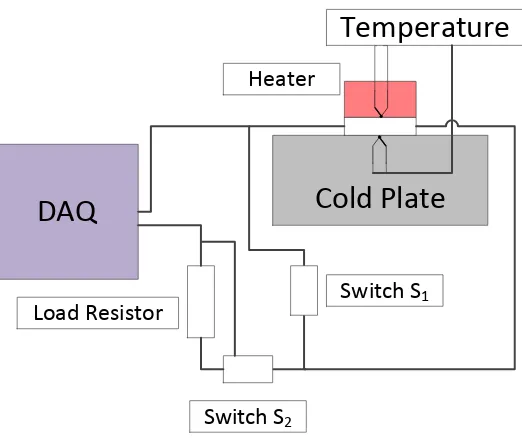
equation. Figure 3.5 shows a schematic of the test setup. A module is attached to a heated

aluminum block, which acts as a heat sink with the help of thermal grease. The other side of the

module is well insulated to maintain adiabatic conditions. The temperature of the aluminum

Page | 37

Figure 3.5: Schematic of the experimental setup for the positive and negative tests showing the flow of heat from and into the module

A current is passed through the module, which produces a voltage and corresponding

temperature difference. The flow of heat into and out of the module depends on the direction of

the current. In our test, when the temperature of the aluminum block was lower than the adiabatic

surface, it was called a positive cycle, and when the temperature of the block was higher, it was

called a negative cycle. All terms with a prime () notation refer to the negative cycle.

The for any term indicates that it is averaged over the bipolar tests. Note that the sign

convention defined in Fig. 3.5 is that positive values for heat flow on the cold side represent heat

flowing into the cold surface, while positive values on the hot side represent heat leaving the hot

surface.

All measurements are taken at a steady state when there is no significant change in voltage and

temperature differences.

Page | 38

In all equations, and . is the ambient temperature.

The components of the heat flow, which can be seen in Fig. 3.6, can be expressed as:

Figure 3.6: Thermal modeling when current is applied in thermal equilibrium [28]

(sum of module Peltier heating and cooling for both current

directions)

Positive Test: Cold Side =

Hot Side =

Negative Test: Cold Side =

Hot Side =

Page | 39

(sum of all module internal conduction heat transfers)

Positive Test: Cold Side =

Hot Side =

Negative Test: Cold Side =

Hot Side =

If is the effective conductance of the module, the surface area of the module, and L the thickness of the module,

then

(3.11)

Positive Test: Cold Side =

Hot Side =

Negative Test: Cold Side =

Hot Side =

Where is the conductivity of the insulation material and is the thickness of the insulation,

Page | 40

Positive Test: Cold Side =

Hot Side = 0

Negative Test: Cold Side = 0

Hot Side =

Where is the conductivity of the aluminum block, is the surface area of the aluminum

block, and is the thickness of the aluminum block,

Let

be denoted as the effective conductance, :

(3.13)

Positive Test: Cold Side = ⁄

Hot Side = ⁄

Negative Test: Cold Side = ⁄

Hot Side = ⁄

(3.14)

Two other sources corresponding to wire conduction and wire joule heating are neglected owing

to very low resistance when compared to the module.

Now, at a steady state, the sum of all expressions is

Page | 41 By manipulating the expression, one can obtain

(3.16)

Let .

In solving for B,

(3.17)

because 0 when the module is in a steady state for both bipolar tests. This

assumption is valid as it represents the temperature of the aluminum block. In both cases, this

temperature is manually controlled.

Thus, we can assume that B 0 for proof of concept testing, but more extensive analysis will

need to be made for full and critical testing.

Let

where A is the correction factor for the equivalent heat losses and C is the overall correction

factor.

(3.18)

Now, solving for α,

(3.19)

But, from the voltage equations of a TEM, we know

and

Hence,

Page | 42 where ̅

By equating Eqns. (3.19) and (3.20), we can calculate the value for conductance:

̅̅̅[ ] (3.21)

The resistance is calculated using the resistive component of voltage and is very straightforward:

̅̅̅ _̅ ̅ _̅̅̅̅ (3.22)

To calculate the dimensionless quantity figure of merit, we use the standard formula

(3.23)

By substituting Eqns. (3.20), (3.21), and (3.22) in (3.23),

[

̅̅̅̅ ]

( ̅̅̅̅ _̅̅̅̅̅)( ̅̅̅̅[ ( ) ( )] ) (3.24)

In solving, we get

̅̅̅ ̅

̅ ̅̅̅ (3.25)

Equations (3.20) - (3.22), and (3.25) fully characterize a thermoelectric device based on voltage,

current, and temperature measurements. This approach is known as the modified Harman method. Note that no heat rate measurement is required, which is typically the case for

steady-state testing methods. Thus, using this approach eliminates the uncertainty of measuring heat

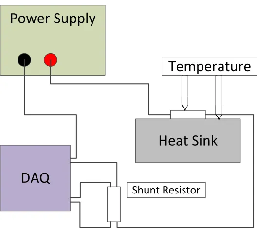
Page | 43 Preliminary experimental setup

The experimental setup consists of a power supply, a shunt resistor, an aluminum heat sink, and

a couple of thermocouples to measure the temperatures. The data from the thermocouples as well

as the current and voltage sensors is recorded with the help of a DAQ board. The block diagram

of the setup is depicted in Fig. 3.7.

Power Supply

Heat Sink

DAQ

Temperature

Shunt Resistor

Figure 3.7: Block Diagram of the experimental setup for Harman method

One of the major advantages of the modified Harman method is the need for only a low current,

which is typically 10% [50] of the short-circuit current of the module. For the comparison test,

the current is set at 0.5A, and varied to check its effect on the properties. A 0.05Ω shunt resistor

is connected in the circuit to assist in the measurement of the current and voltage. Two

Page | 44 Experimental data

To ensure repeatability of the test, a standard procedure was developed. The experimental

procedure was as follows:

 No current was passed for the first 75 seconds on an isothermal module.

 The selected value of the current was passed for 300 seconds.

 No current was passed for the next 300 seconds.

The timed steps above were selected by keeping in mind that the module must reach a steady

state when the measurements are taken. Figure 3.8 shows the display for the voltage and current

versus time for a sample test sequence. The USB DAQ device had a lot of noise in the current

readings, which was dampened before calculating properties.

Figure 3.8: The plots for voltage and current

The data obtained from the DAQ was used to obtain the key module parameters using

Equations (3.20) - (3.22), and (3.25) above and compared with the data from the steady-state

experiments. Table 3.2 shows a comparison of the measured parameters using the two

techniques.

Page | 45

Table 3.2: Comparison of Thermoelectric Module Properties Measured By the Steady-State Approach and Modified Harman approach

Property Measured Modified Harman Method (373K) Steady State (373K)

α (V/K) 0.054 0.044

R (Ω) 2.21 2.42

K (W/K) 0.892 0.63

ZT 0.54 0.47

Temperature correction

For effective comparison of properties with the steady-state method, a temperature correction

must be applied to the modified Harman results. Because the Harman approach was developed

for material testing and adapted for modules, it does not include the temperature gradient

between the thermoelectric pellet and the ceramic face, where the thermocouples are attached to

take measurements. This can be seen in fig. 3.9. This will cause the temperature difference to be

overestimated. To compensate for this, a correction factor needs to be applied to the temperature

readings from the Harman approach.

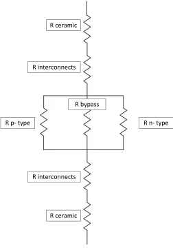
Page | 46 Evaluation of the multiplying factor

The factor can be calculated by considering the module as a set of thermal resistances, as shown

in Fig. 3.10.

Figure 3.10: Thermal resistances in a TEM

Using the standard values of materials available in the literature, we can compute each thermal

Page | 47

Table 3.3: Thermal resistances for a module

Material Length (m) Conductivity

(W/m-K)

Cross-sectional

Area (m2)

Thermal Resistance

(K/W)

Copper 0.00052 385 2.32E-06 0.583

Ceramic 0.00111 22 2.32E-06 21.792

P-type thermoelectric

material

0.00129 1.545 1.10E-06 757.325

N-type thermoelectric

material

0.00129 1.54 1.10E-06 759.784

Solder 0.00005 50 1.10E-06 0.907

We can now calculate the multiplying factor as

( )

( ) . (3.26)

Thus, MF = 0.8946.

Using this multiplying factor, the results from the forward and reverse tests were compared again

Page | 48

Table 3.4: Comparison With Steady-State Results After Correction

Properties Modified Harman (397K) Steady State (397K)

α (V/K) 0.048 0.044

R (Ω) 2.25 2.42

K (W/K) 0.7 0.63

ZT 0.541 0.47

Testing with different temperatures showed