Theoretical and Empirical Contributions to Monetary Policy Analysis

City, University of London Institutional Repository

Citation:

This is the accepted version of the paper.

This version of the publication may differ from the final published

version.

Permanent repository link:

Link to published version:

Copyright and reuse: City Research Online aims to make research

outputs of City, University of London available to a wider audience.

Copyright and Moral Rights remain with the author(s) and/or copyright

holders. URLs from City Research Online may be freely distributed and

linked to.

Theoretical and Empirical Contributions to

Monetary Policy Analysis

Monika Junicke

A thesis submitted in ful…lment of the requirements

for the Philosophy Degree in Economics

City University London

Department of Economics

Contents

1 Welfare Analysis in a Model with In‡ation Persistence and

Non-Zero Steady State In‡ation 18

1.1 Introduction . . . 18

1.2 Literature Review . . . 20

1.3 The Model: Demand Side . . . 22

1.3.1 The Household Optimisation Problem . . . 23

1.3.2 Consumption Index and Consumer Price index . . . 25

1.4 The Model: Supply Side . . . 26

1.4.1 Derivation of the Phillips Curve . . . 30

1.4.2 Price Dispersion . . . 32

1.5 Non Policy Equilibrium and Steady state . . . 33

1.5.1 Non Policy Equilibrium . . . 33

1.5.2 The Steady State . . . 34

1.5.3 Innovations and Calibration of the model . . . 42

1.6 Welfare Loss Function and Welfare Loss Measure . . . 43

1.6.1 Welfare Loss Function using the Hamiltonian Approach . . . 44

1.6.3 Welfare Measure . . . 57

1.7 Analysis of Monetary Policy . . . 59

1.8 Results . . . 63

1.9 Concluding Remarks . . . 68

1.A Consumer Price Index . . . 71

1.B Phillips Curve . . . 73

1.C Central Bank Loss Function . . . 74

1.D Optimal Rules Coe¢ cients . . . 87

2 Estimation of a Small New Keynesian Model with Trend In‡ation for Eastern European Countries 89 2.1 Introduction . . . 89

2.2 Literature Review . . . 92

2.3 The Model . . . 94

2.3.1 Demand Side . . . 95

2.3.2 Firm Optimisation: The Phillips Curve . . . 110

2.3.3 Steady State and Log-linearised Form of the Model . . . 115

2.3.4 Monetary Policy Rules . . . 120

2.4 Model Estimation and Estimation Results . . . 125

2.4.1 Methodology . . . 125

2.4.2 Choice of Prior . . . 129

2.4.3 Estimation Results . . . 135

2.5 Concluding Remarks . . . 162

2.A Data . . . 164

2.C Quantitative Implications of Positive Trend In‡ation . . . 170

3 Impact of Foreign Monetary Policy on Eastern European Coun-tries 175 3.1 Introduction . . . 175

3.1.1 Literature Review . . . 178

3.2 Methodology . . . 181

3.2.1 The reduced-form VAR . . . 182

3.2.2 The Structural VAR . . . 183

3.2.3 BVAR with Gibbs Sampling Estimation . . . 191

3.3 Empirical Analysis and Results . . . 198

3.4 Reconciling the DSGE and VAR Responses . . . 212

3.5 Concluding Remarks . . . 214

3.A Data . . . 216

3.B Model with US, German and EEC data . . . 218

List of Tables

Table 1.1: Calibration of Model Parameters . . . 40

Table 1.2: Hamiltonian Outcomes for Di¤erent Shares of Backward Looking Firms . . . 46

Table 1.3: Structural Parameters of the Hybrid NKPC . . . 55

Table 1.4: Variances and welfare loss under simple policy rules . . . 64

Table 1.5: Variances and welfare loss under optimal policy rules . . . 67

Table 1.6: Optimal rules coec/ cients for linearised and Hamiltonian approach . . . . 88

Table 2.1: Prior Distribution for Large Economy . . . 132

Table 2.2: Prior Distribution for Small Open Economy . . . 133

Table 2.3: Posterior Odd Test for German data . . . 136

Table 2.4: Parameter Estimation Results for Germany . . . 139

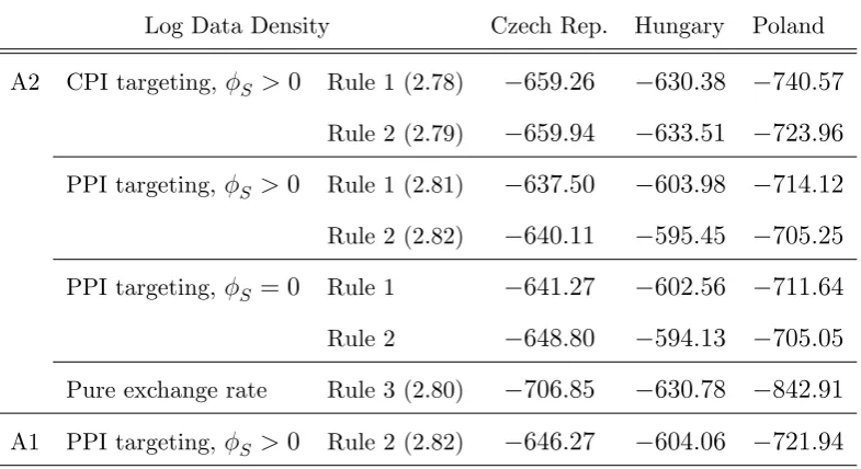
Table 2.5: Marginal Data Densities under Di¤erent Approaches and Monetary Policy Rules Regimes . . . 140

Table 2.6: Posterior Odd Test, hypothesis that the central bank uses a CPI in‡ation targeting . . . 142

Table 2.7: Posterior Odd Test for EEC . . . 143

Table 2.8: Posterior Odd Test for exchange rate targeting . . . 144

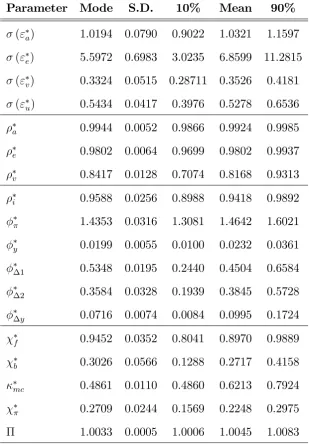
Table 2.9: Parameter Estimation Results for the Czech Republic . . . 145

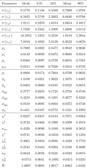
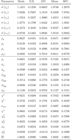
Table 2.10: Parameter Estimation Results for Hungary . . . 146

Table 2.11: Parameter Estimation Results for Poland. . . .147

Table 3.1: Forecasting Error Variance Decomposition for CPI In‡ation . . . 206

List of Figures

Figure 1.1 Pro…t Tree . . . 27

Figure 1.2 Relationship between Steady State In‡ation and Price Dispersion . . . 37

Figure 1.3 Relationship between Steady State Output Gap and In‡ation . . . 40

Figure 1.4 Impulse response functions under simple policy rules . . . 65

Figure 2.1 Multivariate Convergence Diagnostic for Germany . . . 137

Figure 2.2 Multivariate Convergence Diagnostic for the Czech Republic . . . 148

Figure 2.3 Prior and Posterior Distribution for the parameter . . . 149

Figure 2.4 Prior and Posterior Distribution for the parameter _F . . . 150

Figure 2.5 Impulse Responses to a Domestic TFP shock. . . .151

Figure 2.6 Impulse Responses to a Domestic Monetary Shock . . . 153

Figure 2.7 Impulse Responses to a Domestic Producer Cost Push Shock . . . 154

Figure 2.8 Impulse Responses to an Importer Cost Push Shock . . . 155

Figure 2.9 Impulse Responses to a Domestic Preference Shock. . . .156

Figure 2.10 Impulse Responses to a Foreign TFP Shock . . . 157

Figure 2.11 Impulse Responses to a Foreign Monetary Shock . . . 159

Figure 2.12 Impulse Responses to a Foreign Cost Push Shock . . . 160

Figure 2.13 Impulse Responses to a Foreign Preference Shock . . . 161

Figure 3.1 Dynamic E¤ect of a US monetary shock on EEC macroeconomic variables . . . 201

Figure 3.3 Dynamic E¤ect of a US monetary shock on German

and EEC macroeconomic variables . . . 204 Figure 3.4 Contribution of a US monetary policy shock

to the EEC GDP Growth . . . 209 Figure 3.5 Contribution of a ECB monetary policy shock

to the EEC GDP Growth . . . 210 Figure 3.6 Contribution of a US monetary policy shock to the German

and EEC GDP Growth . . . 211 Figure 3.7 Recursive means of the retained Gibbs draws

for (US_Czech Republic) model . . . 221 Figure 3.8 Recursive means of the retained Gibbs draws

for (US_Czech Republic) model . . . 222 Figure 3.9 Recursive means of the retained Gibbs draws

Acknowledgements

I would never have been able to …nish my thesis without the guidance of my

advisors, the help of my friends, and the support of my family.

My …rst and sincere appreciation goes to my supervisor, Prof. Michael

Ben-Gad, for all I have learned from him and for his help and support at all stages of my

doctoral studies. In particular, I thank him for his endless patience and motivation

in guiding me. I also owe my recognition and respect to Prof. Joseph Pearlman

for helping me in gaining focus in my research, and particularly for his suggestions on the …rst chapter of this work. Moreover, I would like to thank all the members

of the Department who supported me during my studies. On a professional as

well as personal level, it gives me great pleasure in acknowledging the help of

Haroon Mumtaz for sharing with me his knowledge of empirical macroeconomics.

Completing this thesis would have been all the more di¢ cult were it not for his

comments and discussion as well as his unbounded moral support.

My greatest gratitude goes to my …ancé Vincenzo Merella, who has always been a great support in all my struggles and frustrations. I thank him for questioning

me about my ideas and helping me think rationally, for listening to me and my

problems and for being here for me at any time when I needed. A big thanks

goes also to Vincenzo’s parents, Adelaide and Alessandro, and to many of my

friends and colleagues: Kristina Baumgarden, Anna Amini, Dorian Quint, Claudia

Markovic, Angeliki Theophilopoulou, Henrique Basso and Ourania Dimakou, to

cite only some. They have always been of comfort and encouragement. Lastly, and most importantly, I would like to thank all my family and dedicate this work to my

Declaration

I grant powers of discretion to the University Librarian to allow this thesis to

be copied in whole or in part without further reference to me. This permission

Abstract

This thesis collects three di¤erent contributions to monetary macroeconomics, covering both theoretical and empirical aspects.

First chapter builds on the DSGE models of New Keynesian tradition, and studies monetary policy around a non e¢ cient steady state. Using a two-stage approach developed by Levine, McAdam, and Pearlman (2007), I show that in the presence of backward looking …rms, the central planner improves social welfare when it allows for a steady state rate of in‡ation marginally above zero.

In the second chapter, I estimate a simple two-country DSGE model to study the behaviour of the Eastern European central banks, obtaining some innovative important results. First, a simple monetary policy rule mimicking an optimal rule together with the assumption about the existence of non-zero steady state rate of in‡ation deliver a signi…cantly better …t to the data. Furthermore, the empirical hypothesis that central banks systematically target CPI in‡ation rather than PPI in‡ation is rejected for all the investigated Eastern European countries (EEC).

Preliminary De…nitions

Actual level of a variable: The nominal value that the generic variable Dt

takes when both stochasticity and (real and nominal) market imperfections are

considered. Written in relative/real terms, the variable is denoted byD~t=Dt=Pt.

Stationary level of a variable: The value that the variable takes when only

(real and nominal) market imperfections are considered. It is denoted by D if in nominal value and byD if in real/relative terms.

Natural level of a variable: The value that the variable takes when only

real market imperfections are considered. It is denoted byDn_.

Deviation of the actual level of a variable from its stationary level:

The ratio between the actual and the stationary level of a variable. It is denoted byD^t Dt=D.

Log-transformation of a variable: The value that obtains by applying

logarithms to the value of the variable. It is denoted by dt logDt. Likewise,

~

Introduction

My research interest focuses on the analysis of monetary policy issues, and covers both theoretical aspects, which I study through Dynamic Stochastic General Equi-librium (DSGE) modelling, and empirical aspects, which I study using Bayesian estimation techniques. My theoretical work, developed in Chapter 1, aims at in-vestigating whether real and nominal frictions may represent a source of trend

in‡ation. My empirical work consists of two exercises. The …rst one, illustrated in Chapter 2, aims at bringing to the data the theoretical predictions delivered by my theoretical analysis. In particular, I investigate whether a DSGE model with non-zero in‡ation performs empirically better than an analogous model ab-stracting from trend in‡ation. This exercise consists a set of three estimations performed in a context with a large economy (represented by Germany) and a small open economy (represented, in turn, by the Czech Republic, Hungary and Poland). The second exercise, described in Chapter 3, extends that performed in Chapter 2 and aims at assessing whether the transmission channel studied there is the most relevant when looking at Eastern European countries (to the three listed

In order to achieve my theoretical goal, I build on the literature of New Key-nesian DSGE models containing real and nominal frictions. The debate regarding economic rigidities has a long history. Phillips (1958) can be considered as a cornerstone for this debate. In the monetary economics literature, many argu-ments suggesting that monetary authorities should take into account the trade-o¤ between in‡ation and output were built upon his empirical …ndings. Monetarist economists criticised this line of reasoning, considering them somehow too “static”.

In their view, the crux of the matter was the assumption that individuals are only able to form in‡ationary expectations based on past in‡ation. This controversy led to the traditional acceleration Phillips curve, characterised by backward looking components. After the famous critique by Robert E. Lucas in 1976, macroeco-nomics was micro-founded, and the resulting theory had individuals making their choices on fully rational decisions. In fact, it was in response to Lucas’critique of ad-hoc modelling that Kydland and Prescott (1982) formulated a theory of micro-founded business cycle models, known as the Real Business Cycle (RBC) theory. This is a general equilibrium models in which the economy responds e¢ ciently to shocks to the total factor productivity that generate ‡uctuations. It is because of

the e¢ ciency of these responses that monetary policy has no real e¤ects on the economy. Their model became an important building block for the New Keyne-sian models (NKM), which represent the class of models that central banks most commonly rely upon at present.

Phillips curve (NKPC) with a simple forward looking component does not corre-spond well with empirical results, as it is unable to capture in‡ation persistence. Having recognised the importance of the in‡ation inertia, economists have been looking for a way to create a Phillips curve that could simultaneously have both forward and backward looking elements. One of the …rst attempts to develop a “two-sided Phillips curve” was Fuhrer and Moore (1995), which used two-period Taylor contracts.

Another approach proposes an indexation of in‡ation. This is possible by using

either the method of static indexation, as suggested by e.g., Yun (1996), or the dynamic one as in Eichenbaum and Fisher (2003) and Christiano, Eichenbaum and Evans (2005). Yun (1996) uses the idea that …rms that cannot re-optimise in a given period, may increase prices in the attempt to anticipate potential in‡ationary phenomena, which they take statically into account at a …xed rate. Static in‡ation can be seen as the long term average rate of in‡ation and, therefore, long term in‡ation inertia is introduced into the model. Similarly, in the model of dynamic indexation from Christianoet al. (2005), …rms that are not allowed to re-optimise may raise prices by adding a fraction of the last observed rate of in‡ation. Both

Nonetheless, the empirical evidence about the importance of the backward looking component in the NKPC delivers ambiguous results. Most of the estimates suggest a hybrid NKPC with a backward looking component. A value of lagged in‡ation should be around 0.3 to 0.5, in line with other empirical …ndings such as Galí and Gertler (1999) and Galí, Gertler, and Lopez-Salido (2001). Benigno and Lopez-Salido (2002) test the Galí-Gertler model on …ve countries in the Euro Area, showing that German …rms behave rationally and, therefore, in‡ation is

strongly forward looking. By contrast, in France, Spain and Italy, the opposite is true. In these countries, …rms are characterized by backward looking price setting behaviour, strongly linking their prices to past conditions. These asymmetries are important as they complicate the determination of unique monetary policy within the Euro Area. Using Bayesian estimation for euro area data and model with NKPC based on Christiano et al. (2005) approach, Smets and Wouters (2003) show, that the forward looking component clearly dominates, however, the backward looking one is also important. Values for both parameters are in line with the …ndings above. Conversely, some authors, e.g., Levine, Pearlman, Perendia, and Yang (2012), show that including habit formation improves the performance

of the model more than a backward looking component of the Phillips curve. For comparison, the estimates for habit formation are usually large: the literature refers to a value around 0.8.

improve social welfare by allowing a steady state rate of in‡ation marginally above zero. In such an environment, there are two forces in the steady state that tend to balance out. On the one hand, given a positive rate of in‡ation, a non-zero price dispersion arises in steady state, decreasing welfare. On the other hand, positive in‡ation causes leisure to decline, and thereby includes a rise in output, bringing it closer to its e¢ cient level. This means that the steady state output gap is lower than it would be in the absence of in‡ation and welfare rises. There is no obvious

analytical solution to the central planner problem, so I solve the model numerically using the Levine-Pearlman Dynare-based system, known as ACES (Analysis and Control of Economic Systems).

My empirical work, developed in Chapters 2 and 3, is based on the Bayesian estimation approach, which I apply to two questions. I estimate a simple two-country DSGE model, similar to Lubik and Schorfheide (2007), with a non-zero steady state in‡ation, to study the behaviour of the Eastern European central banks. The Bayesian analysis, which I carry out using a Metropolis-Hastings al-gorithm, suggests that my model performs better than the benchmark in several aspects. First, I can show that assuming the existence of trend in‡ation, i.e.,

Hungary, and Poland.

Second, I use a Bayesian VAR with economically interpretable structural re-strictions and zero rere-strictions on lags to analyse the transmission channels of external shocks to an extended set of EEC, which also includes Slovakia (along with Czech Republic, Hungary, and Poland). Following Mackowiak (2006), I study to what extent monetary policy shocks originating from the US and from Germany can explain ‡uctuations on Eastern European markets. To carry out the Bayesian inference, I use a Gibbs sampling approach. I …nd that the US monetary policy

Chapter 1

Welfare Analysis in a Model with

In‡ation Persistence and

Non-Zero Steady State In‡ation

1.1

Introduction

In the New Keynesian literature, the long run equilibrium is typically de…ned as a steady state with zero in‡ation. Casual observations however suggest that in‡ation exhibits a non-zero trend, and several recent empirical contributions point out that trend in‡ation plays an important role in shaping many macroeconomic features. In particular, a signi…cant deal of this literature seems to focus on the e¤ects of the existence of trend in‡ation on monetary policy conduct. This chapter attempts to complement these studies, and investigates whether monetary policy may be a possible cause of trend in‡ation. Speci…cally, I seek to …nd an answer to the

In order to explore this idea, I develop a New Keynesian model where a social planner seeking to maximise welfare optimally chooses the level of steady state in‡ation. My model features two key aspects. First, I consider a hybrid Phillips curve, containing both a forward-looking and a backward-looking component, as in Galí and Gertler (1999) and Steinsson (2003). Second, I depart from studying the equilibrium around the e¢ cient steady state of the model and, following Levine, McAdam, and Pearlman (2007), I use the Hamiltonian approach rather than the

traditional linear-quadratic approximation to derive the welfare loss function. As I show and discuss in the next sections of this chapters, both aspects are key in that overlooking either of them would result in the social planner trivially choosing zero steady state in‡ation. That is, the traditional New Keynesian prediction about trend in‡ation results as a particular case of the more general model that I develop in this chapter.

My analysis shows that, around a non e¢ cient steady state, the magnitude of the share of backward looking …rms in‡uences the optimal level of the steady state in‡ation. In particular, the social planner chooses zero in‡ation if just the forward-looking component of the Phillips curve exists. More generally, the presence of a

A natural question that arises in this context is how the welfare loss resulting from the Hamiltonian approach relates to the one obtained by the traditional linear-quadratic approximation. To this aim, I investigate the e¤ect on welfare of the intervention of a central bank (acting as a social planner), introduced using a number of simple and optimal policy rules. In particular, I analyse the individual performance of these rules and their impact on the social welfare in the presence of a TFP shock. I …nd that the presence backward looking component is paramount in

determining the di¤erence in the welfare losses computed using the traditional and the Hamiltonian approach. Such a di¤erence is best observed when simple rules are adopted. In line with the literature, I also …nd that, using either approach and under a common calibration, the pure in‡ation targeting rule performs best, as it lowers signi…cantly more the volatility of in‡ation relative to the other simple rules.

1.2

Literature Review

Despite being a relatively recent feature in monetary economics, trend in‡ation has already been studied in conjunction with a number of issues in this literature. For instance, Ascari (2004) log-linearises the baseline New Keynesian Model (NKM) around an exogenously determined positive steady state in‡ation to argue that

its e¤ects on a variety of di¤erent monetary policy rules.

The material discussed in this chapter relates to a number of articles studying social welfare in the presence of trend in‡ation. For example, Ascari and Ropele (2007) study the optimal monetary policy in a NKM with non-zero steady state in‡ation to point out that the level of trend in‡ation has a strong impact on social welfare. Schmitt-Grohé and Uribe (2007) show that, when one considers positive steady state in‡ation, exogenously given and calibrated to match US data, price dispersion is a …rst order source of social welfare ine¢ ciency. My work di¤ers from

these contributions as the e¤ects on social welfare are investigated with references to a level of in‡ation optimally chosen by a benevolent.

Another branch of the literature that is linked to the analysis developed in this chapter studies trend in‡ation in relation to speci…c aspects on the behaviour of in‡ation itself. In particular, building on the literature modelling trend in‡ation as a random walk without drift (e.g., Cogley and Sargent, 2005Cogley and Sargent (2005); Stock and Watson, 2007), Cogley and Sbordone (2008) …nd that a purely forward looking New Keynesian Phillips Curve (NKPC) with a trend in‡ation is empirically capable to explain a great deal of the observed in‡ation persistence in the US data. As such, trend in‡ation contributes a highly persistent component

to actual in‡ation, from a source that is quite di¤erent from any intrinsic persis-tence implied by the dynamics of price adjustment. My research complements this contribution by investigating whether in‡ation persistence may be an endogenous source, as well as a consequence, of non-zero steady state in‡ation.

linear-quadratic approach. In the benchmark model (see, e.g., Clarida, Galí and Gertler, 1999), welfare loss is a function of in‡ation and output gap. Although, as Steinsson (2003) shows, this traditional method can be applied to a model with built-in in‡ation persistence (with the welfare loss function simply featuring an additional term), the standard linear-quadratic approximation can only be used if small deviations from the e¢ cient steady state are considered. In the e¢ cient steady state, nominal and real frictions are neutralised, hence output is at its

e¢ cient level and, more importantly, in‡ation displays a zero trend. As a result, the traditional approach is unsuitable to deal with my analysis. For this reason, I depart from this literature and use the approach developed by Levine et al. (2007). These authors develop a linear-quadratic approximation around a non e¢ cient steady state, known as the Hamiltonian approach, which I adapt to the analysis of monetary policy with endogenous trend in‡ation and in‡ation persistence. The advantages of this alternative method are that nominal and real frictions need not be eliminated in the steady state (in particular, in‡ation need not display a zero trend), and that the welfare loss function can be derived also for bigger deviations from the steady state.

1.3

The Model: Demand Side

consumer’s dynamic optimisation problem.

1.3.1

The Household Optimisation Problem

The economy consists of a continuum of in…nitely lived households, which all have identical preferences. The representative household maximises the discounted stream of instantaneous utility functions over current and future periods

U =Et

1 X

t=0

t

[U(Ct; Nt)], (1.1)

by optimally choosing, at each date t ₂ [0;₁), Ct consumption units and Nt working hours. The preference parameter ₂ (0;1] is the subjective household discount factor. I assume thatUC >0, UN <0, UCC <0, UN N >0and UC;N = 0. In solving this problem, the household is subject to the budget constraint

Bt+WtNt+Tt+Dt CtPt+Et[Qt;t+1Bt+1], (1.2)

where Et[Qt;t+1] represents the price of the riskless bond held in Bt+1 units,CtPt are consumption expenditures, Wt is the nominal wage, Tt is a lump sum trans-ferand Dt is the net pro…t that the …rms pay to the shareholders (households), which does not a¤ect any other variables in the model.

The Lagrangian that corresponds to the representative agent’s optimisation takes the following form

L=Et

1 X

t=0

t_[U(C

Solving the maximization problem, I obtain the …rst order conditions

@U @Ct

= UC;t tPt= 0, (1.3)

@U @Nt

= UN;t+ tWt= 0, (1.4)

@U @Bt+1

= t+1+ tQt;t+1 = 0, (1.5)

@U @ t

= Bt+WtNt+Tt+Dt CtPt Qt;t+1Bt+1 = 0, (1.6)

where t is the Lagrangian multiplier and can be interpreted as the shadow price of consumption.

Euler Equation

The gross return of a one year riskless bondRt equals the reciprocal of its price

Rt=

1

Et[Qt;t+1]

,

where Et[Qt;t+1] is also known as the dynamic stochastic discount factor. Note

that Rt = (1 +it), whereit is the nominal interest rate. From the condition (1.3) I obtain the conventional stochastic Euler equation

Et

UC;t+1

UC;t

Pt

Pt+1

=Et[Qt;t+1]; (1.7)

Labour Supply

From condition (1.4), I obtain the equation that determines household’s labour

supply

~

Wt =

UN;t

UC;t

; (1.8)

according to which the marginal rate of substitution between labour and consump-tion equals the real wage W~t=Wt=Pt.

1.3.2

Consumption Index and Consumer Price index

I assume there exists a unit continuum of di¤erentiated goods available in the goods market. I abstract from government spending so that all goods are consumed by domestic households. Ctis a composite consumption good, which takes the familiar Dixit-Stiglitz form

Ct=

0 @

1 Z

0

[Ct(i)]

" 1 " _di

1 A

" " 1

; (1.9)

where the parameter " > 1 represents the (constant) consumption elasticity of substitution, and Ct(i) represents the consumption level of good i. As I show in Appendix 1.A, I obtain the demand for an individual consumption good

Ct(i) =

Pt(i)

Pt "

Ct; (1.10)

as a function of its price Pt(i) relative to the price index Pt, of the composite consumption levelCt, and of the elasticity of substitution parameter "t.

for all t, I can rewrite (1.10) to measure production of …rm i Yt(i) =

Pt(i)

Pt "

Yt; (1.11)

which represents the relationship linking individual output to aggregate output and the relative price. Price dispersion in (1.11) is an important source of poten-tial welfare losses in a closed economy. Using equation (1.10), I also obtain an expression for the consumer price index in a closed economy as a function of each

good’s price, formally

Pt=

2 4

1 Z

0

(Pt(i))

1 "

di

3 5

1 1 "

: (1.12)

It is worth mentioning that, in this closed economy model, the consumer price index and the producer price index are identical.

1.4

The Model: Supply Side

In order to obtain the Phillips curve, it is convenient to look at the behaviour of each …rm in the goods markets. The reason is that I assume that only some …rms will set the optimal price as they would under perfect price ‡exibility, while the others will not. Moreover, …rms supply di¤erentiated goods to the markets, and this allow them to have a certain degree of market power. As a result, …rms are not price-takers, but rather incorporate the demand function into their decision regarding how much they should produce.

I closely follow the price setting mechanism in Calvo (1983) and Galí and

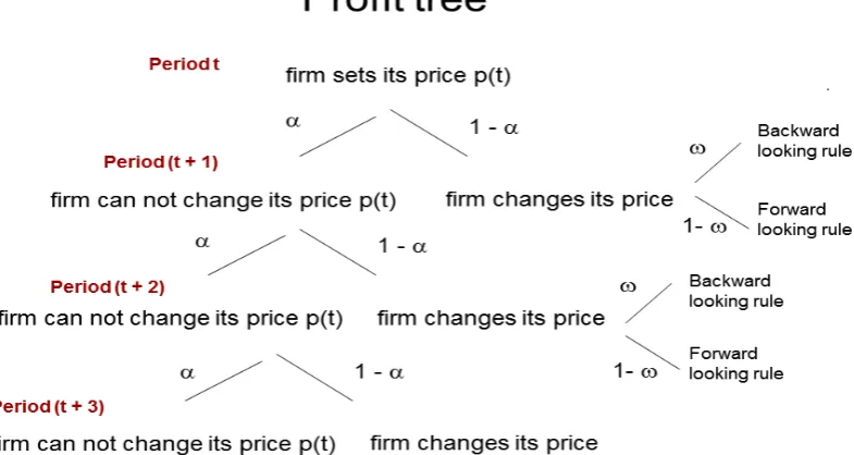
Figure 1.1: Pro…t tree: A share of 1 …rms are allowed to change their prices, from which ! …rms choose a price according rule of thumb.

group of …rms, with measure 1 !, set the price optimally. The complementary measure! set the price according to a rule of thumb. Firms may face two di¤erent situations: i) they are allowed to set their price (with probability 1 ); ii) they are not allowed to do so (with probability ). Hence, at each time t, a measure

(1 !) (1 )set the price optimally, and are labelledf; a measure!(1 )set the price according to a rule of thumb, and are labelled b; …nally, a measure leave the price unchanged, and are labelled s.

Optimal Prices

P_tf(i)to maximise its expected stream of pro…tsGt(i)subject to the technological constraint (represented by its production function)

max

Ptf(i) 1 X j=0 j_E t h

Qt;t+j Ptf(i)Yt+j(i) Wt+jNt+j(i)

i

;

subject to: Yt(i) = AtNt(i); and Yt(i) = Pt(i)

Pt

"

Yt;

(1.13)

where At is total factor productivity, which is common to all …rms. As already mentioned above, assume that the stock of capital is …xed, so labour is the only variable input in the production function, and its demand function given by

equa-tion (1.11). Hence, the …rst order condiequa-tion for this problem is

1 X j=0 j_E t "

Qt;t+j (1 ")Yt+j

P_tf(i)

Pt+j

! "

+"Wt+j P_tf(i)

Yt+j

At+j

P_tf(i)

Pt+j

! "!#

= 0.

De…ning the nominal marginal cost as

M Ct(i) =Wt=At=M Ct; (1.14) and using (1.7) together with the fact that, at time t, j = 0 and so j = 1 and

Q1;1 = 1, I can rewrite this expression to obtain

P_tf(i)Et

" ₁ X

j=0

j jUC;t+j

UC;t

Pt

Pt+j

1

Pt+j "

Yt+j

#

= "

" 1Et

" ₁ X

j=0

j jUC;t+j

UC;t

Yt+jM Ct+j

Pt

Pt+j

1

Pt+j "#

Multiplying both sides by(1=Pt) "

and UC;t yields

~

P_tf(i)Et

" ₁ X

j=0

j j

UC;t+jYt+j

Pt+j

Pt

" 1#

= "

" 1Et

" ₁ X

j=0

j j

UC;t+jYt+jM Cgt+j

Pt+j

Pt "#

;

(1.15)

whereP~_tf(i) = P_tf(i)=Pt is the relative forward looking price andM Cgt=M Ct=Pt is the real marginal cost. This equation can be written in terms of forward looking

price and in‡ation, using Pt+j=Pt = t+j t+j 1 ::: t+1 =

j

Y

k=1

t+k, where

t=Pt=Pt 1 is in‡ation in period t. It therefore holds that

~

P_tf(i) = Jt

Ht

: (1.16)

The variables Jt and Ht are respectively given by

Jt= UC;tYtM Cgt+ Et[( t+1)"Jt+1] (1.17)

and

Ht =UC;tYt+ Et ( t+1)" 1Ht+1 : (1.18)

The expression = "=(" 1) is the constant markup that the …rm charges by exploiting its monopolistic power. Recall that if the …rm faced perfect competition, this markup would disappear and …rms would set their (relative) prices equal to

Rule of Thumb and Staggered Prices

Consider now the!(1 )…rms, labelled b, that set their price at time t. These …rms do so according to a rule of thumb, i.e., by indexing the price to the last observed rate of in‡ation, t 1, yielding

P_tb(i) = t 1Xt 1 =Ptb; (1.19) where Xt 1 denotes the index of the prices set at date t 1. The rule of thumb

in relative terms, using the de…nition of relative prices P~b

t Ptb=Pt and X~t 1

Xt 1=Pt 1, is given by

~

P_tb = t 1

t

~

Xt 1: (1.20)

The new average price set in periodt is then de…ned by

Xt

h

(1 !)P_tf(1 ") +!P_tb(1 ")i

1 1 "

. (1.21)

and equivalently in relative terms by

~

Xt

h

(1 !) ~P_tf(1 ") +!P~_tb(1 ")i

1 1 "

. (1.22)

1.4.1

Derivation of the Phillips Curve

their prices at all so that for them

P_ts(i) = Pt 1; (1.23)

which in relative terms is

~

P_ts(i) = 1

t

. (1.24)

I obtain the Phillips curve representing the supply side of the model by ag-gregating the prices chosen by the di¤erent types of …rms. Hence, from equation (1.12), it follows that

1 =

1 Z

0

Pt(i)

Pt 1 " di = 2 6 4

(1 _Z)(1 !)

0 h

~

P_tf(i)i1 "di+

1 Z

(1 )(1 !)

h

~

P_tb(i)i1 "di+

1 Z

1 h

~

P_ts(i)i1 "di

3 7 5 1 1 " :

To simplify, I assume that all …rms face the same shock and share the same tech-nology. Therefore, all …rms of the same type will set the same price when allowed

to change it. ThereforeP~_tf(i) = ~P_tf and P~_tb(i) = ~P_tb and the Phillips curve is

1 = (1 ) (1 !) P~_tf

1 "

+ (1 )! P~_tb

1 "

+ ( t) " 1

: (1.25)

1.4.2

Price Dispersion

The dispersion between the …rm’s price and the aggregate price level is an

impor-tant source of social ine¢ ciencies. Given that some of the individual prices are staggered and that the aggregate price level changes, the relative prices of individ-ual goods change. Dispersion in relative prices Zt leads to output dispersion that in turn leads to an ine¢ cient level of aggregate production.

Aggregating the individual output across the …rms by using individual produc-tion funcproduc-tion (1.13) yields

Z 1

0

Yt(i)di =At

Z 1

0

Nt(i)di: From the de…nition of aggregate labour: Nt=

R1

0 Nt(i)di, this means that

Nt=

Z 1

0

Yt(i)

At

di:

Multiplying and dividing by Yt, and using equation (1.11)

Nt=

Yt

At

Zt; (1.26)

where Zt is a measure of relative price dispersion, given by

Zt=

Z 1

0

Yt(i)

Yt

di=

Z 1

0

Pt(i)

Pt "

di:

Together with equation (1.25), the measure of price dispersion can be rewritten as

Zt = (1 ) X~t "

Note that Yt 6=

R1

0 Yt(i)di; using a composite consumption together with the

market cleaning condition for closed economy, I get the composed expression for output

Yt=

0 @

1 Z

0

[Yt(i)]

" 1 " _di

1 A

" " 1

:

As Schmitt-Grohé and Uribe (2007) demonstrate, relative price dispersion is bound-ed below by Zt 1. Additionally, price dispersion can be disregarded in the …rst order approximation of the model. Woodford (2003) and Schmitt-Grohé and Uribe (2007) also show that, given a steady state with zero in‡ation ( = 1), price dis-persion is deterministic and follows a AR(1) process, and as such does not have any real e¤ect.

1.5

Non Policy Equilibrium and Steady state

After a brief discussion about a non-policy equilibrium of this model, in this sec-tion I introduce a deterministic environment around a steady state with non-zero in‡ation, and I compare it to a steady state with zero in‡ation, illustrating the similarities and pointing out the di¤erences.

1.5.1

Non Policy Equilibrium

Assume that the instantaneous utility function is time-separable and takes the

form

U(Ct; Nt) =

C_t1

1

N_t1+

where and are positive parameters, interpretable as constant relative risk aversion (CRRA) coe¢ cients, which determine the elasticities of substitution of consumption and labour supply. The marginal utility of consumption and marginal disutility of labour are given respectively by

UC;t =Ct and

UN;t= Nt:

For a closed economy, the equilibrium is speci…ed by Ct = Yt and Bt = 0, so that the Euler equation takes the form

Et

"

Yt+1

Yt

Pt

Pt+1 #

=Et[Qt;t+1]. (1.29)

1.5.2

The Steady State

In the literature, it is common to assume that in‡ation in steady state equals zero (i.e., the gross rate of in‡ation is = 1). However, as I demonstrate in this section, a moderate long run in‡ation, that is, a steady state non-zero in‡ation, can improve social welfare. This fact is exploited by the central planner in the case that ! > 0, i.e., in a model with (some) backward looking agents, as described in more details in Section 1.6.1. Prior to this, it is necessary to de…ne the

In short, I can summarise the overall e¤ect of a non-zero steady state in‡ation as follows. On the one hand, positive in‡ation generates greater price dispersion

Z, so the aggregate output tends to decrease. On the other hand, as I show below, positive (small) in‡ation leads to an increase in real marginal labour cost. Since wages are ‡exible, marginal cost equals real wage, thus positive (small) steady state in‡ation leads to a higher real wage. Higher real wage has both income and substitution e¤ects. The income e¤ect that follows from an increase in real

wages will cause an increase in both leisure and consumption. Therefore, labour supply decreases. However, because of the higher wage, workers also substitute their leisure with labour. A rise in the labour input induces an increase in aggre-gate output. Hence, as I will demonstrate below the e¤ect of in‡ation on output is determined by two countervailing forces, a positive e¤ect generated by induc-ing higher real wages and a negative e¤ect generated by inducinduc-ing greater price dispersion.

From the Euler equation in the steady state, using equation (1.29), it follows that the market discount factor equals its subjective counterpart

=Q; (1.30)

where is steady state in‡ation. Therefore, it holds that if in‡ation in steady state is non-zero, the discount factor Q is lower than the subjective household’s discount factor .

steady state real wage

W = UN

UC

: (1.31)

From the supply side, using equations (1.20), (1.22) and (1.25), all …rms allowed to change the prices set them equally, as a function of the level of steady state in‡ation, formally

Pb =X

and

Pf =X;

where:

X = 1 ( )

" 1

1

! 1

1 "

: (1.32)

Note that, if = 1, then also the new and old prices equal the CPI, and therefore the model delivers unit relative prices. In the case that the steady state in‡ation is positive, the nominal prices increase steadily. It follows from the de…-nition of the price index that this aggregator averages new and unchanged prices, so it holds that P < X = Pf _{= P}b_{. Thus, the new nominal price grows more} than the price index, which is pulled down by the lower prices chosen in the last periods, making the new relative price larger than one, formally

Pf = P

f

P >1:

The fact that zero in‡ation implies that all relative and nominal prices equal one

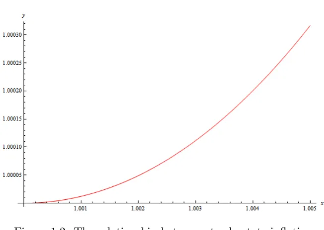
Figure 1.2: The relationship between steady state in‡ation (horizontal axis) and price dispersion (vertical axis).

the price dispersion is above one. Using equation (1.27) in steady state, price dispersion is a function of the new price and in‡ation, formally

Z = (1 )X

"

1 " : (1.33)

Price dispersion is directly related to in‡ation as long as the gross rate of in‡ation

is close to one. Figure 1.2 shows that a higher in‡ation generates larger steady state price dispersion. Solving (1.16) for marginal costs in terms of the rate of in‡ation yields

M C = 1 1

"

1 " 1 P

f_{: (1.34)}

markup, otherwise the real marginal costs also depend on the level of the steady state in‡ation. On one hand, if is close enough to one, the marginal costs are directly related to the rate of in‡ation. On the other hand, with higher steady state in‡ation, real marginal costs decrease.A small increase in the steady state in‡ation leads to higher real marginal costs. Given that the real marginal costs are proportional to the real wage, gross in‡ation slightly higher than 1 leads to an increase in the real wage.

Inserting the equality M C =W into equation (1.34) together with (1.32) and rearranging, I get

W = 1 1

"

1 " 1 X: (1.35)

At the …rm-level, for the production function and for the aggregate production function in steady state

Y (i) =N(i)

and

Y = N

Z:

The wedge between aggregate output and labour is the reciprocal of the price dispersion.

Finally, the level of output in steady state can be expressed as a function of steady state in‡ation

Y = 1

1 +

2

4 1 " 1

1

"( +1) " 1

(1 )1+ (1 " 1₎

(1 "_{) (1} " 1_{) (1} "₎

# 1

+

:

The steady state level of output (1.36) di¤ers from the natural level of output

Yn_{. The natural level of output arises when all prices are ‡exible (i.e., = 0), so} all …rms set their prices equal. For this reason, at the natural level of output all prices are equal to the consumer price index, i.e., Pt(i) = Pt, and it follows that

X =Pf _=Pb _{= 1. The natural level of output itself can be expressed as}

Yn= +1 :

Note that, in the case of zero in‡ation, steady state output equals its natural level, because any e¤ects from the presence of nominal distortions are neutralised by the equality of nominal and real prices for all …rms. Therefore, the output gap, de…ned as the ratio between actual and natural level of outputY~ =Y =Yn_{, equals} one.

In the case of non-zero in‡ation, the output gap is instead given by

~

Y =

2

4 1 ( )

" 1

1

! " " 1( +1)

(1 )1+ (1 " 1) (1 "_{) (1} " 1_{) (1} "₎

3 5

1 +

:

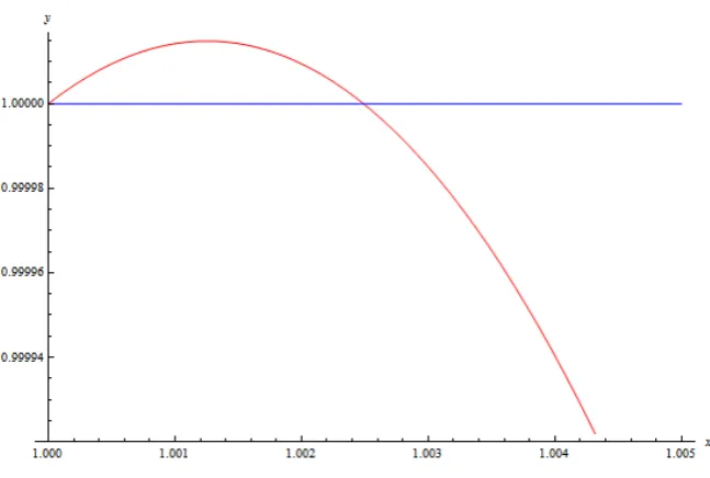
Figure 1.3 shows that a small level of in‡ation can increase steady state output

over its natural level. However, higher in‡ation is distortionary and leads to a negative output gap, i.e., Y <~ 1.

Figure 1.3: The relationship between steady state in‡ation (horizontal axis) and steady state output gap (vertical axis).

M P N equals the marginal rate of substitution M RSC;N.

The wedge between steady state output and its e¢ cient level therefore re‡ects the wedge between the marginal product of labourM P N =Y =N and the marginal rate of substitutionM RSC;N = UN=UC, which can be illustrated using (1.35) in conjunction with (1.36)

Y N =

UN

UC

(1 " 1_{) (1} "₎

(1 "_{) (1} " 1₎: (1.37)

1:5 inverse intertemporal elasticity of substitution

1 inverse elasticity of labour supply

0:99 subjective discount factor

2=3 parameter of price stickiness

" 4 elasticity of substitution between goods Table 1.1: Calibration of the model parameters

captured by the mark-up . Note that assuming perfect competition,"_{! 1}leads to a zero mark-up, where = 1.

Rotemberg and Woodford (1998) emphasise that the aim of the policy maker is to stabilise the economy around the e¢ cient level of outputYe

t . To this aim, they approximate the welfare of the representative household around the e¢ cient level of output. As mentioned above, nominal distortions in steady state disappear if in‡ation equals one. Real distortions generated by monopolistic competition can be o¤set by introducing employment subsidies that increase the output up to the desired e¢ cient level. Using equation (1.37), it follows that it is su¢ cient to introduce an output subsidy with rate such that (1 ) = 1. In other words, the subsidies can be expressed as = " 1 > 0, and the higher the elasticity of substitution,i.e., the lower the markup, the lower the subsidies required to obtain the e¢ cient level of output.

1.5.3

Innovations and Calibration of the model

In the last section, I described my model in its deterministic, perfect foresight,

steady state. In what follows I study the behaviour of the model in a stochastic environment where the source of uncertainty is represented by shocks to total factor productivity (TFP). The TFP innovation At measures the aggregate technology process, which (log-linearised) follows the stochastic AR(1) process

^

at= a^at 1+ a;t;

where a^t (logAt logA) denotes the deviation, in log terms, of TFP from its steady state value, _{a 2} [0;1) is the autocorrelation parameter, and

a i:i:d:(0; 2a) is a white noise shock.

In assigning numerical values to the structural parameters, I closely follow the

literature. Table 1.1 reports the calibrated values for the parameters of the model. The parameter is the inverse of the intertemporal elasticity of substitution (IES), and the elasticity is usually assumed to take values between 0.5 and 1. I choose

= 1:5so that the IES equals0:67. The labour disutility parameter is set equal to one, in accordance with the estimates from Smets and Wouters (2003).

Each time period in this model corresponds to a quarter of a year, hence

1.6

Welfare Loss Function and Welfare Loss

Mea-sure

There are several linear-quadratic approaches in the literature to approximating the welfare loss function. Generally, a linear-quadratic approach uses the …rst order approximation of the structural equations to obtain a second order approximation of the utility function to represent the social welfare function. There is an extensive literature devoted to the analytical derivation of the welfare loss function. This paper provides a welfare based analysis to measure the e¤ectiveness of di¤erent

monetary policy rules comparing two di¤erent approaches: the traditional linear-quadratic approach and the Hamiltonian approach.

The …rst approach is based on Levine, McAdam, and Pearlman (2007) and their Hamiltonian two-stage linear-quadratic approach. I show that, for a Ramsey planner and in the presence of backward looking …rms, it is desirable to impose a non-zero steady state rate of in‡ation.

In their work, Levine et al. (2007) develop a two-stage Ramsey policy, where in the …rst stage a steady state in line with a social planner allocation is found and corresponds to a best possible deterministic outcome. In the second stage, a monetary policy rule for a stochastic environment is determined, which leads to the lowest possible welfare loss (and therefore the closest to the steady state value

derived in the …rst stage). In this case, however, it is not possible to derive an analytical solution for the welfare loss function, so the model is solved numerically using Dynare/ACES software.

Steins-son (2003) and similar to Rotemberg and Woodford (1999), and enables me to compare my results with the numerical solution. Following Rotemberg and Wood-ford (1999), the second order approximation of the welfare loss function is derived together with the …rst order approximation of the equilibrium conditions. Two conditions are necessary to derive an accurate second order approximation of the welfare using this method. First, the real distortions following from monopolistic competition have to be eliminated by assuming labour subsidies, thus allowing

only for small distortions. Therefore, in the steady state, the output gap is zero and the model is log-linearised around its e¢ cient level. Second, the approxima-tion has to be calculated in a closed neighborhood of zero steady state in‡aapproxima-tion, so that in the steady state the price distortions are eliminated.

1.6.1

Welfare Loss Function using the Hamiltonian

Ap-proach

In this section, I explain how the welfare loss is calculated using the two-stage approach by Levine et al. (2007). In the …rst stage, the social planner chooses a steady state in‡ation level, which maximises steady state welfare. In the second stage, welfare in a stochastic environment around the …rst-stage steady state is maximised.

Generally, the goal of the central bank’s monetary policy is to maximise a social welfare function , which consists of the discounted stream of the households’ utility over the current and the future periods

=

1 X

t=0

t_U

where Ut is the instantaneous utility function of the representative household. Using (1.28), the nonlinear optimisation problem for the Ramsey planner is de…ned by

=E0 1 X t=0 t 2 4C j1 t 1 Z 1 0

N_tj(i) 1 + di

!1+ 3

5;

where C_tj =Ct for all households j, given the assumption that all household have identical preferences and resources. An individual j supplies N_tj labour in total, assuming that to each …rm i it supplies equal amount of labour N_tj(i). Given (1.26), the Ramsey planner problem can be rewritten as

=E0 1 X

t=0

t

"

C_tj1

1 1 1 + Yt At Zt 1+ #

and is maximised subject to the structural conditions (1.25), (1.16), (1.17), (1.18), (1.20), (1.22) and (1.27). In this …rst stage, it is only necessary to …nd the …rst

order conditions in a deterministic steady state. Thus, only the optimal steady state is identi…ed.

Using a Dynare based MATLAB software package called ACES (Analysis and Control of Economic Systems), and assuming that in‡ation is the instrument con-trolled by the central bank, the steady state of this problem is identi…ed as a non-zero steady state in‡ation when ! > 0. As illustrated in Figure 1.3, a mod-erate steady state rate of in‡ation leads to output rising above its natural level (e.g., Y > Yn_{) and it can be shown that the social planner chooses a positive} rate of steady state in‡ation whenever ! >0. Recall from Section 1.5.2 that, for

! W N C =Y

0 1 0:75 0:891299 0:891299 251:5670 0:3 1:00006 0:750002 0:8913 0:8913 251:5657 0:5 1:00013 0:750006 0:891302 0:891302 251:5656 0:8 1:00052 0:750021 0:891311 0:891308 251:5657

Table 1.2: Hamiltonian steady state outcomes for di¤erent shares of backward looking …rms.

that output may rise above its natural level. Therefore, there is a certain trade o¤ between these two e¤ects, where the positive e¤ects outweigh the negative ones if

in‡ation is positive but very small.

Given (1.38), social welfare in the steady state is measured as

= 1

1 U(C; N): (1.39)

As it is shown in Table 1.2, the social welfare rises as the value of the backward looking parameter!is increased.1 _{The higher the share of backward looking}

com-panies, the higher the trend in‡ation chosen by the social planner. Higher in‡ation leads to a higher real wage and an increase in labour because the substitution e¤ect dominates the income e¤ect. Although output increases with the level of steady state in‡ation, its rise is lower than that of labour, due to the additional price dispersion that higher in‡ation generates.

From the equations in Section 1.5.2, it is straightforward to notice that the

1_{For reference, note that the level of welfare generated in an e¢ cient level of output is}

steady state outcomes are not directly in‡uenced by the parameter!. As a result, one might be tempted to conclude that the social planner may choose steady state in‡ation independent of this parameter. However, Table 1.2 clearly points towards the opposite direction: the optimal social planner decision is a¤ected by the magnitude of the fraction of backward looking …rms. Zero in‡ation is optimally chosen only when all …rms are forward looking, and this also represents the steady state with the lowest level of output and welfare. As the fraction of backward

looking …rms increases, both in‡ation and welfare grow. This is suggestive of a positive ! being bene…cial for the economy.

One possible rationale for this …nding relies on the price dispersion being, under certain conditions and o¤ steady state, a negative function of !.2 In the presence of backward looking …rms, in fact, the social planner would exploit this negative link by letting in‡ation reach an optimal positive level in the steady state. In particular, the larger!, the higher the optimal steady state in‡ation. As explained above, a positive in‡ation increases welfare through the marginal costs channel, and decreases it by raising price dispersion. For any given! >0, it is then possible to …nd a level of positive in‡ation that would result in better outcomes than a zero

in‡ation (both in transition and, eventually, in the steady state). Suppose that the social planner attempted to impose the same level of steady state in‡ation

2_{More precisely, I can rewrite (1.27) as}

Zt= (1 ) (1 !) Ptf=Pt "

+! P_tb=Pt "

+ Zt 1 "t;

from which it follows that Ptf > Ptb entails dZt=d! < 0. This means that, whenever forward looking …rms (f) set a higher price than their backward looking counterparts (b), price dispersion is inversely related with the fraction ofb…rms. The conditionP_tf > Pb

with a lower !. Then, the fraction of forward looking …rms would possibly be su¢ ciently large to command a high price dispersion, whose negative e¤ects may overcome the positive ones due to the rise in labour supply. Of course, the social planner could not possibly exploit this channel to improve welfare when!= 0, as the forward looking NKPC would lack any in‡ation inertia.

The aim of the second stage of the Hamiltonian approach is to derive an accu-rate linear-quadratic approximation in a stochastic environment around a steady state level identi…ed in the …rst stage. Calculating the …rst order Taylor

approx-imation (log-linearisation) of the …rst order conditions and the constraints, to-gether with the second order Taylor approximation of the Hamiltonian with the Lagrangian problem, delivers a quadratic approximation of the utility expressed in terms of the state variables. In the presence of non-zero in‡ation, an analytical derivation of this function is not possible. Thus, at this point, I merely compare the welfare loss function obtained from analytical solution of simple linear-quadratic approach with the numerical results obtained directly using ACES.

1.6.2

Analytical Approximation of the Welfare Loss

Func-tion

Because the analytical derivation of the welfare function around a steady state with non-zero in‡ation is not possible, I compare my numerical result, obtained using the Hamiltonian approach described in previous section, with the result derived from the traditional approach, analogous to the one implemented by Steinsson (2003). This method is based on a linear-quadratic approach using the …rst order

the welfare function. The approximation of the second order of the welfare function is detailed in the appendix. The analytical welfare loss function also proves useful for a derivation of the optimal monetary policy under commitment.

I study the model in the neighborhood of its non-stochastic perfect-foresight steady state. There are two points worth mentioning. First, without any further assumptions, this steady state does not achieve the long run e¢ cient level of output because of the presence of nominal and real distortions. In particular, non-zero in‡ation in the steady state generates a degree of price dispersion that, together

with the …rms’ monopolistic power, implies lower output. This causes problems when calculating the second order approximation of the welfare, and therefore these distortions have to be neutralised, as discussed in Section 1.5.2.

Log-Linearisation

To derive analytically the loss function around the steady state with zero in‡a-tion, it is necessary to approximate the structural equations of the model in a close neighborhood of the model’s steady state. The log-linearisation of a generic variable Dt around its steady state valueD can be generally expressed as

Dt=DelogDt=D =DelogDt logD =De(dt d) =De

^

d _{D 1 + ^d} t :

However, some of the structural equations are linear in their logs so I can write directly logDt = dt. This holds for the Euler equation (1.29), whose log-linearisation is

yt=Et yt+1+

1

with % = log and where pt+1 pt t+1 and it = log (Qt;t+1). Assuming

that the variables do not deviate much from their steady state values, the Euler equation can be written as a deviation from its steady state level as

^

yt =Et y^t+1+

1

( t+1 ^{t) , (1.40)

where I employ the de…nitionsp^t+1 p^t t+1 and^{t [log (Qt;t+1) log (Q)].3

It is clear from (1.40) that, in a closed economy, the real interest rate,it t+1, is

pinned down by the real output growth rate. Hence, if prices are fully ‡exible and …rms are fully rational, central bank intervention modi…es the nominal interest rate, it. This change is fully anticipated by …rms that, by setting their prices accordingly, induce a proportional shift in the in‡ation rate t+1. If prices are

not fully ‡exible and/or …rms are not fully rational, then changes in the nominal interest rate induced by the central bank may have real e¤ects, as prices do not respond proportionally to variations in the nominal interest rate. As a result, in‡ation only partially responds to the central bank intervention, and real output growth, yt yt 1, also changes. The …nal result is that the Euler equation holds

with a modi…ed real rate of interest and a modi…ed degree of output growth.

For this reason, it is important to introduce the concept of natural equilibrium, where all …rms are fully rational and may adjust their prices every period. Denote the log-linearisation of the generic variableDt in its natural level as dnt logDtn. Following the de…nition of the natural level of a variable, I can also rewrite the log-linearised Euler equation in terms of the output gap (the deviation of the real variables from their natural levels), in turn de…ned as the log of the ratio between

3_{Note that since the steady state level of in‡ation is set to be zero, we can write^}

actual output and natural output, and denoted byy~t =yt ytn. Using (1.40) yields

~

yt=Et[~yt+1]

1

Et[it t+1 rnt]; (1.41) where rn

t is the Wicksellian natural rate of interest and it holds that rtn = %+

Et ytn+1 . For future reference, I also express (1.41) as a deviation from the

steady state level, formally

~

yt =Et[~yt+1]

1

Et[^{t t+1 ^rnt]: (1.42) In this case,r^_tn is the deviation of the Wicksellian natural rate of interest from its steady state level, and it holds that ^rn_t = Et ynt+1 .

Additionally, the log-linearisation of the labour supply delivers the relationship between the real wage, labour supply and output

^

wt= ^nt+ ^yt: (1.43)

Furthermore, as I describe in Appendix 1.B in more detail, the supply curve shows how in‡ation reacts to variations in real marginal costs as well as future and past in‡ation. I rewrite this as

with the parameters

= +!(1 (1 ))

f

= = ; b =!=

mc = (1 !) (1 ) (1 )= ;

where 0 < f_; b_;

mc < 1 and >1. Notice that, when ! 1, f + b = 1. Hence, in‡ation is a function of the convex combination of future and past in‡ation.

The measure of price dispersion in (1.27), log-linearised around the zero in‡a-tion steady state, delivers the AR(1) process

zt= zt 1;

which, as discussed in Schmitt-Grohé and Uribe (2007), is purely deterministic up to the …rst order, and does not have any real e¤ect on the rest of the model.

Similar to the Euler equation, the Phillips curve can also be rewritten in terms of the output gap. As mentioned earlier, in the natural state of the economy …rms can reset their prices in each period. Since I assume that all …rms are identical, they will all choose the same price, which equals the aggregate price level. Therefore, all relative prices in the natural level of output equal one.

Formally, it is straightforward to see that the natural level of the relative price (in logarithms) equals the real marginal cost in the natural level mcn

from its steady state level

c

mcn_t = 0: (1.45)

This is because the real marginal cost always equals the mark up, which does not deviate from its steady state level. Log-linearisation of equation (1.14), together with (1.8), yields

c

mct= ^nt+ ^yt at: (1.46)

Additionally, log-linearisation of (1.26), together with the fact that z^t can be dis-regarded, delivers

^

nt= ^yt at:

Inserting this back into (1.46), yields the real marginal cost

c

mct= ( + ) ^yt (1 + )at:

Combining the last expression with (1.45) delivers the natural level of output

^

y_tn= (1 + )

( + )at; (1.47)

and I can therefore express the the relationship between the marginal cost and output gap as

c

mct mcc n

t = ( + ) (^yt y^nt) (1 + )at+ (1 + )at:

Rearranging, and employing the de…nition of the output gap y~t = ^yt y^nt, yields

c

Plugging this equation into (1.44) delivers a hybrid NKPC in terms of the output gap, that is log-linearised around a steady state equilibrium with zero in‡ation

t = fEt[ t+1] + b t 1+ ~yt. (1.49) The parameter = mc( + ) > 0 is the slope of the Phillips curve expressed in terms of the output gap, and re‡ects the relationship between in‡ation and output.

Following Steinsson (2003), I consider four di¤erent values of the backward looking parameter !. The values for the composed parameters under these values of!are shown in Table 1.3. The …rst row corresponds to the standard NKPC with a purely forward looking component, as postulated by most contributions to the literature (e.g., Woodford, 2003). The second row corresponds to the values in the Galí-Gertler estimation for a rule of thumb model.4 As in Steinsson (2003), I refer to the third row as amidway case, where half of the …rms are rational, and half of them follow a rule of thumb. The fourth row correspond to a model with a large share of backward looking …rms and is a good proxy for the Fuhrer-Moore (1995) model. Even when omega is set this high, the Phillips curve is both forward and backward looking, with a slightly higher weight on the latter component. However, the curve becomes very inelastic to changes in the output gap.

Assuming that all …rms are purely backward looking, i.e., ! _! 1, does not directly reduce the Phillips curve to an acceleration Phillips curve, since f

!

=(1 + ). However, Steinsson (2003) shows that taking the limit ! _! 1,

4_{Galí and Gertler (1999) test empirically this hybrid NKPC and argue that, depending on}

! f b

0 0:99 0 0:43

0:3 0:68 0:31 0:21 0:5 0:57 0:43 0:12 0:8 0:45 0:55 0:04

Table 1.3: Structural parameters of the hybrid

NKPC for di¤erent shares of backward looking …rms.

the equation (1.49) has a unique bounded solution in which t = t 1. Hence, if

all …rms are backward looking, the price index in period t simply equals the price index in period t 1, and it holds that f; b; _{! f}0;1;0_g. In this case, the Phillips curve is vertical, which implies the absence of a trade-o¤ between output and in‡ation.

Welfare Loss Function for a Model with Zero Steady State In‡ation

Using the technique described in Rotemberg and Woodford (1999) and Steinsson (2003), and assuming that output is on its e¢ cient level in steady state, the an-alytical derivation of the second order approximation of the objective function is straightforward and is described in more technical details in Appendix 1.C.

Ignoring terms higher than the second order and those independent of policy, the welfare loss function can be approximated by

0 = E0

1 X

t=0

t 2

t +

2

where , y and are functions of the structural parameters of the model. In contrast to the traditional loss function derived by Rotemberg and Woodford (1999) for a model with purely forward looking NKPC, this expression contains the relative weight on the in‡ation growth ‡uctuation term = 1_{!=(1 !),}

which is positively related to the parameter !. That is, the larger the fraction of backward looking …rms, the higher the welfare loss caused by a ‡uctuation in the rate of in‡ation (relative to the level of in‡ation), since the share of prices based

on past information is relatively larger. However, this e¤ect is twofold, because a higher share of backward looking …rms also leads to higher in‡ation persistence, and therefore to smaller changes in in‡ation growth.

The relative weight on output gap ‡uctuations is increasing in and , and given by y = (1= ) (1 ) ( + )=". These two parameters govern the wedge between marginal rate of substitution and marginal product of labour, which measures the level of ine¢ ciency in the economy. The value of y is also decreasing in and ", which in turn govern the weight of output gap ‡uctuations relative to in‡ation ‡uctuations. With the calibration given in Section 1.5.3, the term varies positively with the parameter !. The relative weight on in‡ation growth strengthens as the value of ! is raised, since @2 =@!2 > 0, although it should be noted that increasing in‡ation persistence also implies a decreasing value of squared in‡ation growth deviation.

As long as approaches 1, the average welfare loss can be written as the unconditional expected average welfare loss

The traditional loss function can be found as a special case of (1.50) by imposing

! = 0, which leads to = 0. This loss function corresponds the one derived by Woodford (2003) or Galí (2008), formally

0 = [varf g+ yvarfy~g]: (1.51) In the literature, most contributions opt for this more conservative loss func-tion, even when (1.50) would possibly be the most suitable one, i.e., when the

model actually presents backward looking components (see, e.g., Clarida, Galí and Gertler, 1999).

In the next section, I compare the social welfare loss obtained using the Hamil-tonian approach from Section 1.6.1 with that resulting from the generalised loss function (1.50).

1.6.3

Welfare Measure

The welfare loss can be rewritten in terms of a compensating di¤erential, a mea-sure of how much households should be compensated in order to neutralise the welfare loss. To calculate the compensating di¤erential between two regimes, I use the de…nition of welfare given in (1.38). In this paper, the compensating di¤eren-tial is calculated as a di¤erence between the welfare obtained using the analysed monetary policy rule and the steady state value.

Generally it holds that the analysed rule generates welfare

=

1

X _t

which is compared with the benchmark welfare = 1 X t=0 t

U(C_t; N_t):

I am looking for a consumption compensating di¤erential that equates welfare to its analogous . Formally

1 X

t=0

t_U(C

t; Nt) =

1 X

t=0

t_{U((1 )C}

t; Nt): Putting the speci…c utility function (1.28), welfare reads

= 1 X t=0 t "

((1 )C_t)1 1

N_t1+

1 +

#

;

which can be expressed as

= + (1 )1 1

1 X t=0 tC 1 t 1 :

Solving for the compensating di¤erential, and using the term C =

P1

t=0

t Ct1 1

as the welfare following directly from consumption, I obtain

= 1

C

+ 1

1 1

When compared to the steady state value, welfare is given by

= 1

1 U C; N