1
Performance Analysis of Wells Turbine Blades Using the
1
Entropy Generation Minimization Method
2 3
Ahmed S. Shehata1, 3*, Khalid M. Saqr2, Qing Xiao 1, Mohamed F. Shehadeh 3, 4
Alexander Day1 5
6
1) Department of Naval Architecture, Ocean and Marine Engineering, University of
7
Strathclyde, Glasgow G4 0LZ, U.K
8
2) Mechanical Engineering Department, College of Engineering and Technology
9
Arab Academy for Science Technology and Maritime Transport, P.O. 1029 AbuKir, Alexandria,
10
EGYPT
11
3) Marine Engineering Department, College of Engineering and Technology
12
Arab Academy for Science Technology and Maritime Transport, P.O. 1029 AbuQir, Alexandria,
13
EGYPT
14
* Corresponding Author: Ahmed S. Shehata, E-mail address:
15
16 17
ABSTRACT 18
Wells turbine concept depends on utilizing the oscillating air column generated over
19
marine waves to drive a turbine. As a matter of fact, previous researches on the
20
performance analysis of such turbine were based on the first law of thermodynamics
21
only. Nonetheless, the actual useful energy loss cannot be completely justified by the
22
first law because it does not distinguish between the quantity and the quality of energy.
23
Therefore, the present work investigates the second law efficiency and entropy
24
generation characteristics around different blades that are used in Wells turbine under
25
oscillating flow conditions. The work is performed by using time-dependent CFD
26
models of different NACA airfoils under sinusoidal flow boundary conditions.
27
Numerical investigations are carried out for the incompressible viscous flow around the
28
blades to obtain the entropy generation due to viscous dissipation. It is found that the
29
value of second law efficiency of the NACA0015 airfoil blade is higher by
30
approximately 1.5% than the second law efficiency of the NACA0012, NACA0020 and
31
NACA0021 airfoils. Furthermore, it is found that the angle of attack radically affects
32
the second law efficiency and such effect is quantified for NACA0015 for angle of
33
attack ranging from -15o to 25o.
34
Keywords: Wells turbine; entropy generation; NACA airfoils; sinusoidal wave; CFD.
2 NOMENCLATURE
36
A Cross-sectional area of cylinder (m2)
B Cord of cylinder (cm)
f cycle frequency (Hz)
D
F In-line force acting on cylinder per unit length (gf)
KE Kinetic Energy (W/K)
L Blade Chord (m)
p Pressure field (Pa)
gen
S local entropy generation rate (W/m2K)
G
S Global entropy generation rate (W/K)
𝑆𝑖𝑗 Mean strain rate
t
S Thermal entropy generation rate (W/m2K)
V
S Viscous entropy generation rate (W/m2K)
o
T Reservoir temperature (K)
i
u Reynolds Averaged velocity component in i direction (m/s)
V Instantaneous Velocity (m/s)
a
V highest speed of axial direction (m/s)
o
V Initial velocity for computation (m/s)
rev
W Reversible work
Viscosity (Kg/ms)
𝜇𝑡 Turbulent viscosity
Density (Kg/m3)
𝜎𝜖, 𝜎𝑘 The turbulent Prandtl numbers for 𝜿 and 𝜺 respectively
uiuj
Reynolds stress tensor 373
1. INTRODUCTION
39 40
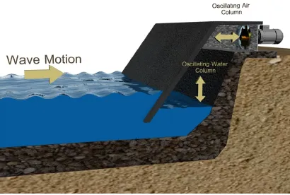
The major challenge facing oscillating water column systems is to find efficient
41
and economical means of converting oscillating flow energy to unidirectional rotary
42
motion, for driving electrical generators. A novel resolution for such challenge is the
43
Wells turbine [1-4], see figure 1(a, b) due to its simple and efficient operation. The
44
Wells turbine has already been applied in practice to gain energy from marine waves. In
45
the past two decades, experimental research of Wells turbine has mainly focused on
46
improving the turbine performance with emphasis on the overall operational
47
characteristics. The airfoils sections that are used in Wells turbine have been extensively
48
investigated in aeronautical applications. However, the operating conditions in Wells
49
turbine are completely different from such of the aeronautical applications. In Wells
50
turbine, the rotor contains multiple blades, which are confined by a shroud aiming at
51
harnessing the flow momentum to drive the rotor with the maximum torque. The flow
52
physics in such situations are still having several issues to investigate; besides, the
53
dynamical complexity resulting from an oscillating water column driven by random
54
irregular marine waves.
55
Second law analysis of energy conversion systems has become an important tool
56
for optimization and development during the past decade. In Fact, the second law of
57
thermodynamics is more reliable than the first law of thermodynamics analysis due to
58
the limitation of the first law efficiency in a heat transfer engineering systems as well as
59
heat transfer, mass transfer, viscous dissipation, etc. Moreover, the second law can be
60
used as the sources of entropy generation [5, 6].Consequently, This work utilizes
time-61
dependent numerical models of different NACA four-digit series blade profile under
62
oscillating flow conditions. Numerical investigations are carried out for the flow around
63
Wells turbine blades using sinusoidal wave boundary conditions to perform as realistic
64
characterization as possible of the flow field upstream and downstream of the turbine
65
during the passage of the wave. The Gouy–Stodola theorem [7] has been used to
66
compute the second law efficiency from the results of the numerical simulations. This
67
theorem postulates the difference between reversible and actual works in any
68
thermodynamic system which is the entropy generation in such system, as discussed
69
later in section 4. Such theorem is the foundation for the entropy generation
4
minimization method proposed by Bejan [8] to optimize finite size thermodynamic
71
systems.
72
A thorough literature survey has revealed that the second law analysis of the
73
oscillating flow around wells turbine has not been conducted before. However, this
74
section briefly reviews the most relevant studies to accentuate the scope of the present
75
work. In a number of previous studies, it is concluded that the delay of stall onset
76
contributes in improving Wells turbine performance. This delay can be achieved by
77
setting guide vanes on the hub near the rotor[9].
78
As far as the running and starting characteristics of the Wells turbine are
79
concerned, Wells turbine with 3D guide vanes are superior to those with 2D guide vanes
80
or without guide vanes[10, 11]. Furthermore, the presence of end plates is investigated
81
experimentally and numerically by [12, 13] where they conclude that the Wells turbine
82
with end plates is superior to those of the original Wells turbine(which was investigated
83
also in this work) because the peak efficiency and the stall margin increases by
84
approximately 4% and its characteristics are dependent on the size and position of end
85
plate.
86
87
Three dimensional numerical simulations are performed by Thakker et al [14] in
88
order to analyze the performance of a Wells turbine with CA9 blade profile, a maximum
89
efficiency of 70% is obtained. Moreover, Kim et al [15] uses numerical simulation to
90
study the effect of the blade sweep on the performance of a Wells turbine using either
91
NACA0020 or CA9 blade profiles. They were found that the performance of the Wells
92
turbines with NACA0020 and the CA9 blades are influenced by the blade sweep. As the
93
optimum rotor shape for a NACA0020 blade, a blade sweep ratio 35% is identified to
94
deliver the optimum performance. In general, the overall turbine performance for the
95
NACA0020 is better than such of the CA9, Also, Takao et al [16], presents
96
experimentally the suitable choice the sweep ratio of 0.35 for the cases of CA9 and
97
HSIM 15-262123-1576. In another study [17], the characteristics of a Wells turbine
98
with NACA0021 constant chord blades are investigated. They find from the numerical
99
results that the wakes behind the turbine blades merge rigorously in the portion of radius
100
ratio from 0.45 to 1.0, which leads the turbine to stall.
5
One and two stage Wells turbines involving symmetric airfoils and
Non-103
Symmetric airfoils are investigated by Mohamed [18, 19]. Numerical optimization
104
procedure has been carried out to optimize the performance of the turbine as a function
105
of the non-dimensional gap between the two rotors. It is leading to an optimal value of
106
the non-dimensional gap (The distance between the two stages / the blade chord) near
107
0.85 when considering the operating range. Moreover, the Evolutionary Algorithms are
108
used to estimate the optimum shape with an increase of efficiency (by 2.1%) and of
109
tangential force coefficient (by 6%), compared to the standard NACA 2421, as well as
110
the one-stage the optimum shape with an increase of efficiency (by 1%) and of
111
tangential force coefficient (by 11.3%), compared to the standard NACA 0021.
112 113
On the other hand, the hysteretic characteristics of monoplane and biplane have
114
been studied in a number of studies [20-26]. The objective of such works is mainly to
115
investigate the aerodynamic losses of Wells turbine. It is found that for the biplane, the
116
hysteretic behavior is similar to that of the monoplane at lower angles of attack, but the
117
hysteretic loop similar to the dynamic stall is observed at higher angles of attack.
118
Exergy analysis is performed using the numerical simulation for steady state biplane
119
Wells turbines [27] where the upstream rotor has a design point second law efficiency
120
of 82.3% although the downstream rotor second law efficiency equals 60.7%.
121 122
Most of the researchers who have investigated the performance of different
123
airfoils design and different operational condition have analyzed the problem using only
124
the parameter of first law of thermodynamic that lead to several contradicting
125
conclusions that can be observed, for example, in [28].This shows that the use of two
126
twin rotors rotating in the opposite direction to each other is an efficient means of
127
recovering the swirl kinetic energy without the use of guide vanes. On quite the
128
opposite, a contra-rotating W-T which is investigated in [29], it is found to have a
129
lower efficiency than a biplane or monoplane W-T with guide vanes. Another example,
130
we can observe this contradiction also in the comparison between the performances of
131
the Wells turbines in four different kinds of blade profile (NACA0020; NACA0015;
132
CA9; and HSIM 15-262123-1576). Which, the blade profile of (NACA0020) have the
133
best performance according to the result of [16, 30], but, according to the result of [31]
6
the blade profile of (NACA0015) achieve best result. Finally, the rotor geometry
135
preferred was the blade profile of (CA9) according to the result of [32, 33].
136
It is essential to look at the second law of thermodynamic to form a deeper
137
understanding, since it has shown very promising result in many applications, like wind
138
turbine in [34-38], Radial Compressor Stage [39], pipe flow [40], thermal power plants
139
[6], and Rotating disk [5].
140 141
The objective of the present work is essentially to investigate the entropy
142
generation, due to viscous dissipation, around Wells turbine airfoils in
two-143
dimensional unsteady flow configurations. The research aims to use the entropy
144
generation due to viscous dissipation around a Wells turbine blade as very
145
sensitive judged parameter on the turbine performance for any change in terms
146
of the operating condition (the flow Reynolds number up to 2.4×10⁵ and the
147
airfoil angle of attack from -15 to 25 degree), the blade design (four different
148
airfoils) and flow direction (sinusoidal wave with compression and suction
149
cycle). This work is limited to four airfoils namely NACA0012, NACA0015,
150
NACA0020 and NACA0021. These airfoils are common to use in Wells turbine
151
applications.
152 153
2. MATHMEATICAL MODEL AND NUMERICAL APPROACH
154 155
The mathematical model consists of the governing equations of turbulent
156
incompressible unsteady flow in two-dimensional generalized coordinates, which can be
157
written in vector notations as[41]:
158
Continuity:
0 i i u x t (1) 159
RANS:
i j
j i j ij i j j i j j j i i
i uu
x x u x u x u x x p u u x t
u
3 2 160 (2) 161
and turbulent flow is modeled using the Realizable k-e model, Transport equation of
162
turbulent kinetic energy (k)
163
164
𝜕
𝜕𝑡 𝜌𝑘 + 𝜌 𝜕
𝜕𝑥𝑖 𝑈𝑖𝑘 = 𝜕
𝜕𝑥𝑗 𝜇 + 𝜇𝑇 𝜎𝑘
𝜕
7
(3)
165
Specific dissipation rate equation is:
166 167 168 (4) 169 170 Where 171 172 173 (5) 174 Where 175 176 177
and the vorticity tensor
178 179
where u is the Reynolds averaged velocity vector. The present study adopts one and
180
two-equation turbulence models to close the Reynolds stress term
uiuj
of the181
RANS equation [42] as shown in the following section. The transport equations of such
182
models can be found in turbulence modeling texts such as [43].The second law of
183
thermodynamic defines the net-work transfer rate W as [8]:
184
gen o rev T S
W
W (6)
185 186
It is possible to express the irreversible entropy generation in terms of the
187
derivatives of local flow quantities in the absence of phase changes and chemical
188
reactions. The two dissipative mechanisms in viscous flow are the strain-originated
189
dissipation and the thermal dissipation Which correspond to a viscous and a thermal
190
entropy generation respectively [39]. Thus, it can be written,
191
th V gen S S
S (7)
192
𝜕
𝜕𝑡 𝜌𝜀 + 𝜌 𝜕
𝜕𝑥𝑖 𝑈𝑖𝜀 = 𝜕
𝜕𝑥𝑗 𝜇 + 𝜇𝑇 𝜎𝜀
𝜕
𝜕𝑥𝑗 𝜀 + 𝐶1𝜌𝑆𝜀− 𝐶2𝜌 𝜀2 𝑘 + 𝜈𝜀
𝐶1= 𝑚𝑎𝑥 0.43, 𝜂
𝜂 + 5 , 𝐶2= 1.9
𝐶𝜇 = 1
𝐴0+ 𝐴𝑠 𝑈∗ 𝑘 𝜀
𝐴0 = 4.0 , 𝑈∗ = 𝑆𝑖𝑗𝑆𝑖𝑗 + Ω𝑖𝑗Ω𝑖𝑗 , 𝐴𝑠 = 6 cos
1
3 𝑎𝑟𝑐𝑐𝑜𝑠 6𝑊 , 𝑊 =
8 𝑆𝑖𝑗𝑆𝑗𝑘𝑆𝑘𝑖
𝑆3
Ω𝑖𝑗 =
1 2
𝜕𝑢𝑖 𝜕𝑥𝑗 −
8
In incompressible isothermal flow, such as the case in hand, the thermal
193
dissipation term vanishes. The local viscous irreversibilities therefore can be expressed
194 as: 195 o V T
S (8)
196
where is the viscous dissipation term, that is expressed in two dimensional Cartesian
197
coordinates as [39]: 198 2 2 2 2 x v y u y v x u
(9)
199
and the global entropy generation rate is hence expressed as:
200
y x V G S dydxS (10)
201
and finely the second law efficiency is defined as :
202 G S S KE KE (11) 203
where 2
2 1
V KE 204
but the efficiency in first law of thermodynamics ( )is defined as:
205 206
𝜂𝑓 = 𝑁𝑒𝑡 𝑂𝑢𝑡𝑝𝑢𝑡 𝑇𝑜𝑡𝑎𝑙 𝑤𝑜𝑟𝑘 𝐼𝑛𝑝𝑢𝑡
207
2.1 Numerical Model Details 208
The computational domain is discretized to Cartesian structured finite
209
volume cells using GAMBIT code. Drichlet boundary conditions are applied on
210
the domain for the solution of momentum and continuity equations. The
211
application of such boundary condition types [21, 44-46] matches the
Green-212
Gauss cell based evaluation method for the gradient terms used in the solver
213
(ANSYS FLUENT). Numerous tests accounting for different interpolation
214
schemes used to compute cell face values of the flow field variables, the
215
variables of governing equation which are velocity and pressure, as well as
216
convergence tests have been undertaken. The second order upwind interpolation
217
scheme is used in this work because it yields results which are approximately
218
(12)
(13)
9
similar to such yielded by third order MUSCL scheme in the present situation. It
219
is also found that the solution reaches convergence when the scaled residuals
220
approaches 1×10⁻⁵. At such limit, the flow field variables holds constant values
221
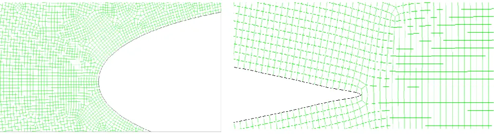
with the application of consecutive iterations. Figure (2); show the dimensions
222
of whole computational domain and location of airfoil. Figure (3) show the grid
223
distribution near the wall of the airfoil.
224
The axial flow of Wells Turbine is modeled as a sinusoidal wave in this
225
simulation. Therefore, Inlet boundary conditions are set to change as time. In
226
order to apply the inlet boundary condition, inlet velocity with periodic function
227
(see figure 4) is generated as follows.
228
𝑉 = 𝑉𝑜 + 𝑉𝑎(sin 2 𝜋 𝑓 𝑡)
229
where t is time period 6.7 seconds are set as one period in this simulation
230
considering to the literature survey [22, 23, 33]. Time step is set as 0.00009
231
second in order to satisfy CFL (Courant Friedrichs Lewy) [47] condition equal
232
to 1. the sinusoidal wave condition create various Reynolds number up to
233
2.4×10⁵ and this maximum value which is taken from many references such as
234
[13, 18, 20-23, 25, 48, 49]. Regarding the angle of attack, it covers wide range of
235
angles of attack in both directions (positive and negative) but it doesn’t need
236
more than this value because the stall condition [50].
237 238 239 240
2.2 Numerical Model Validation 241
In order to ensure that the numerical model is free from numerical errors,
242
several grids are tested to estimate the number of grid cells required to establish
243
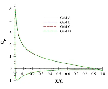
a grid-independent test. Table 1 shows the specifications of different grids used
244
in such test. Figure 5 shows the pressure coefficient (Cp) distribution on the
245
upper and lower surfaces of the airfoil as computed by the four grids. Grid C and
246
D have the same result, but the latter one required less time. So, Grid C is
247
chosen to conduct the analysis presented hereafter.
248
Many turbulence models are used to model the oscillating flow around
249
the object in order to determine the model which gives the best agreement with
250
10
experimental data adopted from [51]. The best result for S-A, k SST and
251
the Realizable kmodel but the latter one required less time [52]. As For the
252
near-wall treatment in both K-epsilon and S-A models have used the log law of
253
the wall but for k-omega models have used y plus less than one. This
254
experimental data for unsteady forces acting on a square cylinder in oscillating
255
flow with nonzero mean velocity are measured [51] where the oscillating air
256
flows are generated by a unique AC servomotor wind tunnel. The generated
257
velocity histories are almost exact sinusoidal waves. The measured unsteady FD 258
is computed from the Morison equation for the in-line force acting on the
259
cylinder per unit length:
260
U C A U U BC
FD D ~D
2
1
261
where U dU dt and the non-dimensional coefficient
D
C~ is the inertia
262
coefficient of the unsteady in-line force. This non-dimensional coefficient is
263
evaluated depend on [53, 54].
264
This data is the most experimental data that have available information for the
265
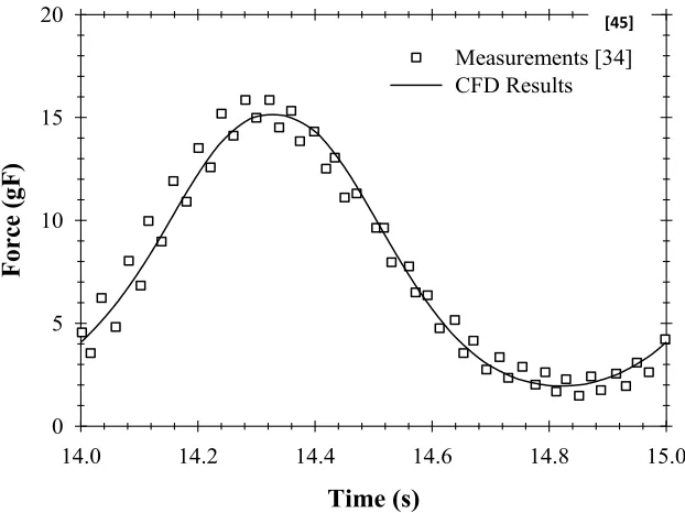
sinusoidal flow condition to validate our work; therefore, it is adopted in the
266
following simulation cases. Figure 6 (a), (b) show an excellent agreement
267
between measured drag force from reference and calculated drag force from
268
CFD at two different frequency.
269 270
3. RESULTS AND DISCUSSION
271
3.1 Evaluation of the second law efficiency of different NACA airfoils 272
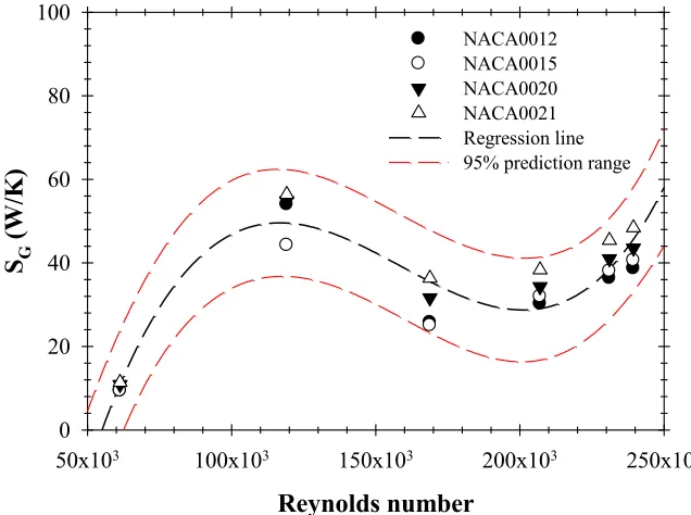
The numerical simulations are used to obtain local entropy viscosity
273
predictions of the different airfoil sections. Figure 7(a) and (b) highlight the
274
entropy behavior when a flow is accelerating in compression and suction cycle.
275
Consequently, the entropy generation ratio various with the Reynolds number at
276
certain angle of attack equal to 2 degree. The change of Reynolds number values
277
is due to using sinusoidal wave boundary conditions. At low values of Reynolds
278
number the stall condition occur at small value of angle of attack[50]. Hence, 2
279
degree angle of attack is chosen to avoid the stall condition.
280
11
The Reynolds number is calculated from equation (14). Otherwise, the value
281
of Reynolds number in this study can be controlled by the value of velocity while
282
keeping the other parameters constant.
283
VL
Re
284
The Reynolds number has radical effect on the entropy generation. This is
285
obvious in the accelerating flow in compression and suction cycle in Figure 7 (a,
286
b), where Reynolds number increase from 6×10⁴ to 1.2×10⁵. As a result, the global
287
entropy generation rate (i.e. integral) has increased correspondingly for more than
288
two folds of all airfoils. However, when Reynolds number has increased further to
289
1.7×10⁵ (2×10⁵ for NACA0012 at compression cycle) the global entropy
290
generation rate exhibited unintuitive values ranging from 50% less to 40% lower
291
than the corresponding value at Reynolds number equal to 1.2×10⁵ for all airfoils.
292
The reason behind such phenomena can be attributed to the nonlinear complexity
293
of the viscous dissipation term (equation 9) where both the square of mean rate of
294
strain and velocity divergence contributes to the local viscous irreversibilities.
295
This phenomenon suggests that possible existence of critical Reynolds number at
296
which viscous irreversibility takes minimum values. At high Reynolds number
297
(greater than 2×10⁵) the change in velocity value, see equation 14, is smaller than
298
low Reynolds number. Where, at 120000 Reynolds number the velocity equal to
299
17.5 m/s, then it increases to 24.8 m/s at 170000 Reynolds number (41%increase
300
rate). After that, it reaches to 200000 Reynolds number with velocity equal to 30.3
301
m/s (22%increase rate). On the other hand, at high Reynolds number (230000) the
302
velocity equal to 33.8 m/s (10%increase rate). Then, at 240000 Reynolds number
303
the velocity reach to maximum value equal to 35.04 m/s (3%increase rate), see
304
Figure 4. This leads to smaller change in flow field and entropy generation. The
305
last one was dependent on velocity analysis.
306 307
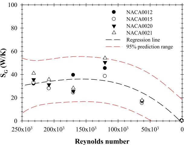
However, in figure 8 (a, b) for decelerating flow in compression and suction
308
cycle when Reynolds number, in Figure (8, a), is decreased further to 1.2×10⁵ the
309
global entropy generation rate exhibited unintuitive values ranging from 94%
310
(NACA0021, NACA0020) less to 59% (NACA0015) and 15% for (NACA0012)
311
12
higher than the corresponding value at Reynolds number equal to 1.7×10⁵. For
312
decelerating flow in suction cycle the global entropy generation rate, at Reynolds
313
number equal to 1.2×10⁵, exhibited unintuitive values ranging from 135%
314
(NACA0012) less to 83% (NACA0020) and 68% (NACA0021, NACA0015)
315
which is higher than the corresponding value at Reynolds number equal to
316
1.7×10⁵. Then, when Reynolds number is decreased further to a minimum value
317
the global entropy generation rate is decreased also to minimum value and not
318
equal to zero. From figure 7 and 8, at maximum Reynolds number, the
319
NACA0012 give lower entropy generation rate than other airfoil. From figure 9, it
320
is concluded that the NACA0015 give lower maximum value for the global
321
entropy generation rate than other airfoil in both cycles. The NACA0015 airfoil
322
section gives less average value ranging from 20% less to 10% of the global
323
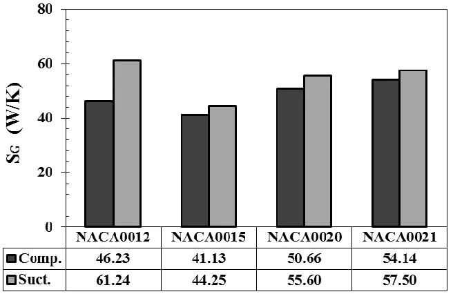
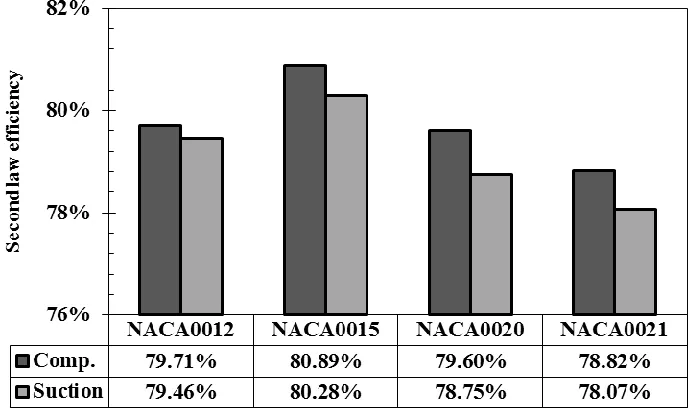
entropy generation rate during the sinusoidal wave cycle see figure 10. To confirm
324
these results we have made a comparison between the second law efficiency for
325
four different airfoils at compression and suction cycle (figure 11) and also for the
326
total average efficiency during the sinusoidal wave cycle (figure 12), NACA0015
327
gives best efficiency when it is compared with other airfoils in both compression
328
and suction cycle and therefore in total sinusoidal wave cycle ranging from 2%
329
less to 1%. In four different airfoils and at certain angle of attack, the efficiency
330
for compression cycle higher than suction cycle ranging from 1% less to 0.3%.
331
Equation (17) is defining the exergy value, which can be written as:
332
G
S KE Exergy 333
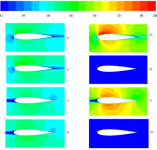
Contours of Exergy around the blade of NACA0015 for angle of attack 2 degree at
334
different time and different velocity along the sinusoidal wave can be seen in figure (13)
335
that the positive value of velocity refers to compression cycle and the negative value
336
refers to suction cycle. From this figure it can be observed that as the velocity increase
337
the value of exergy around the blade increase, otherwise, the leading and trailing edge
338
always have the lowest value, but at compression cycle the area around the trailing edge
339
has lower value than the leading edge, and in the suction cycle the area around the
340
leading edge has lower value than trailing one.
341
342
13
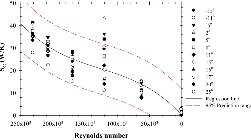
3.2 Effect of the angle of attack on entropy generation 343
The increase of angle of attack has a direct effect to the entropy generation in
344
the flow over the airfoil which is similar to the effect of Reynolds number.
345
However, as shown in figure 14(a) and (b), NACA0015 airfoil has a different
346
entropy generation signature for different angles of attack listed in table 2. For
347
accelerating flow in compression cycle, Figure 14 (a) at Reynolds number equal to
348
1.2×10⁵ the maximum value of global entropy generation rate occurs due to 2
349
degree angle of attack but the minimum value of it occurs due to -15 degree angle
350
of attack. The 17 degree angle of attack gives maximum global entropy generation
351
rate at 1.7×10⁵ Reynolds number, and the minimum value occurs due to -11
352
degree at the same Reynolds number. Finally, at Reynolds number equal to
353
2.3×10⁵ and 2.4×10⁵ the maximum global entropy generation rate occurs due to 17
354
degree and the minimum value occurs due to 5 degree.
355 356
The trend of global entropy generation rate at suction cycle is different
357
from the compression cycle at various angles which can be seen in figure 14 (b).
358
For decelerating flow in suction cycle at Reynolds number equal to 1.7×10⁵, the
359
maximum global entropy generation rate occurs at 5 degree angle of attack and the
360
minimum value occurs due to 25 degree. For Reynolds number equal to 1.2×10⁵
361
the maximum global entropy generation rate occurs due to 2 degree angle of attack
362
and the minimum value due to 25 degree. Low angles of attack around zero, both
363
positive and negative direction have higher global entropy generation rate and
364
lower entropy efficiency except at 17 degree so we can note that there is
365
unexpected increase in the value of global entropy generation rate accompanied by
366
a lack of the second law efficiency, see figure 15 and 16. As For angle of attack
367
from -5 to 5 degree the entropy efficiency for compression cycle higher than the
368
suction cycle ,but when the angle of attack increase in both directions the
369
efficiency for suction cycle exceeds the compression cycle, see figure 17. At same
370
angle of attack but in different direction, the positive direction gives higher
371
efficiency than the negative one. For example, the second law efficiency for 5
372
degree higher approximately 0.5% than -5 degree and approximately 0.1%
373
between 11 and -11 degree and finally 0.3% between 15 and -15 degree.
14 375
4. CONCLUSIONS
376
Second law analysis of Wells turbine requires accurate estimation of flow
377
irreversibilities around the turbine blades. Two-dimensional incompressible unsteady
378
flow simulations of different airfoils reveals that the geometry and the operating
379
conditions have radical effects on the global entropy generation rate in the flow around
380
turbine airfoil. The main conclusions are summarized as follows.
381
1- The relationship between the Reynolds number and the global entropy generation
382
rate haven’t a direct correlation but when compare between four airfoils at certain
383
angle of attack the maximum global entropy generation rate occurs at Reynolds
384
number of 1.2×10⁵ and at 1.7×10⁵ (2×10⁵ for NACA0012 in compression cycle)
385
less than halved.
386
2- NACA0015 gives less global entropy generation rate and higher efficiency
387
compare with other airfoil.
388
3- The efficiency for four different airfoils in compression cycle is higher than
389
suction cycle at 2 degree angle of attack. But when the angle of attack increase,
390
the efficiency for suction cycle increase also more than the compression one.
391
4- At zero and low angle of attack we have higher global entropy generation rate than
392
at high angle of attack.
393
5- From the study of the behavior of four different airfoils, NACA0015 isn’t the best
394
airfoil in all condition .For examples, at maximum Reynolds number NACA0012
395
gives less global entropy generation rate and NACA0020 create the minimum
396
value, so it is a good concept to create an optimum design airfoil gives better
397
result than NACA0015.
398
6- In general the global entropy generation rate due to viscous dissipation is a very
399
sensitive indicator for airfoils behavior at any change in design parameters, the
400
operating condition and also being affected by flow direction.
401 402
5. Acknowledgements 403
The authors would like to acknowledge the support provided by the Department of
404
Naval Architecture, Ocean and Marine Engineering at Strathclyde University and the
15
Department of marine Engineering at Arab Academy for Science, Technology and
406
Maritime Transport.
407 408
6. REFERENCES 409
410
[1] T.J.T.e.a. Whittaker, The Queen's university of Belfast Axisymmetric and
Multi-411
resonant Wave Energy Converters, Trans. ASME. J. Energy Resources Tech., 107
412
(1985) pp. 74-80.
413
[2] T.J.T.a.M. Whittaker, F. A. , Design Optimisation of Axisymmetric Tail Tube
414
Buoys, in: IUTAM, Symposium on Hydrodynamics of Ocean Wave Energy
415
Conversion, Lisbon,July., 1985.
416
[3] T.J.J. Whittaker, McIlwain, S. T. and Raghunathan, S. , Islay Shore Line Wave
417
Power Station, Proceedings European Wave Energy Symposium., Paper G6, Edinburgh.
418
(1993).
419
[4] S. Raghunathan, Theory and Performance of Wells Turbine, Queen's University of
420
Belfast, Rept. WE/80/13R (1980).
421
[5] M.M. Rashidi, M. Ali, N. Freidoonimehr, F. Nazari, Parametric Analysis and
422
Optimization of Entropy Generation in Unsteady MHD Flow over a Stretching Rotating
423
Disk Using Artificial Neural Network and Particle Swarm Optimization Algorithm,
424
Energy, 55 (2013) 497-510.
425
[6] S.C. Kaushik, V.S. Reddy, S.K. Tyagi, Energy and Exergy Analyses of Thermal
426
Power Plants: A Review, Renewable and Sustainable Energy Reviews, 15 (2011)
1857-427
1872.
428
[7] A. Bejan, Entropy Generation Minimization: The Method of Thermodynamic
429
Optimization of Finite-Size Systems and Finite-Time Processes, Taylor & Francis,
430
(1995).
431
[8] A. Bejan, Entropy Generation Minimization- The New Thermodynamics of Finite‐ 432
Size Devices and Finite‐Time Processes, Applied Physics Reviews, (1996).
433
[9] L.M.C. Gato, R. Curran, The Energy Conversion Performance of Several Types of
434
Wells Turbine Designs, Proceedings of the Institution of Mechanical Engineers, Part A:
435
Journal of Power and Energy, 211 (1997) 133-145.
436
[10] T. Setoguchi, Effect of Guide Vane Shape on the Performance of a Wells Turbine,
437
Renewable Energy, 23 (2001) 1-15.
438
[11] M. Takao, T. Setoguchi, T.H. Kim, K. Kaneko, M. Inoue, The Performance of a
439
Wells Turbine with 3D Guide Vanes, International Journal of Offshore and Polar
440
Engineering, 11 (2001) 72-76.
441
[12] M. Mamun, Y. Kinoue, T. Setoguchi, K. Kaneko, A.K.M.S. Islam, Improvement af
442
the Performance of the Wells Turbine by using a Very Thin Elongated Endplate at the
443
Blade Tip, in: the 3rd BSME-ASME International Conference on Thermal Engineering,
444
ASME, Dhaka, Bangladesh, 2006.
445
[13] M. Takao, T. Setoguchi, Y. Kinoue, K. Kaneko, Wells Turbine with End Plates for
446
Wave Energy Conversion, Ocean Engineering, 34 (2007) 1790-1795.
447
[14] A. Thakker, P. Frawley, E.S. Bajeet, Numerical Analysis of Wells Turbine
448
Performance Using a 3D Navier Stokes Explicit Solver, in: International Offshore and
449
Polar Engineerbtg Conference, Stavanger, Norway, 2001.
16
[15] Tae-Hun Kim, Yeon- Won Lee, Ill-Kyoo Park, Toshiaki Setoguchi, C.-S. Kang,
451
Numerical Analysis for Unsteady Flow Characteristics of the Wells Turbine, in:
452
International Offshore and Polar Engineering Conference, The International Society of
453
Offshore and Polar Engineers, Kitakyushu, Japan, 2002, pp. 694-699.
454
[16] T. Setoguchi, M. Takao, K. Itakura, M. Mohammad, K. Kaneko, A. Thakker,
455
Effect of Rotor Geometry on the Performance of Wells Turbine, in: The Thirteenth
456
International Offshore and Polar Engineering Conference, The International Society of
457
Offshore and Polar Engineers, Honolulu, Hawaii, USA, 2003, pp. 374-381.
458
[17] T.S. Dhanasekaran, M. Govardhan, Computational Analysis of Performance and
459
Flow Investigation on Wells Turbine for Wave Energy Conversion, Renewable Energy,
460
30 (2005) 2129-2147.
461
[18] M.H. Mohamed, G. Janiga, D. Th´evenin, Performance Optimization of a Modified
462
Wells Turbine using Non-Symmetric Airfoil Blades, in: Turbo Expo 2008: Power for
463
Land, Sea and Air GT, ASME, Berlin, Germany, 2008.
464
[19] M.H. Mohamed, Design Optimization of Savonius and Wells Turbines, in,
465
University of Magdeburg,Germany, Germany, 2011.
466
[20] Y. Kinoue, T.H. Kim, T. Setoguchi, M. Mohammad, K. Kaneko, M. Inoue,
467
Hysteretic Characteristics of Monoplane and Biplane Wells Turbine for Wave Power
468
Conversion, Energy Conversion and Management, 45 (2004) 1617-1629.
469
[21] M. Mamun, Y. Kinoue, T. Setoguchi, T.H. Kim, K. Kaneko, M. Inoue, Hysteretic
470
Flow Characteristics of Biplane Wells Turbine, Ocean Engineering, 31 (2004)
1423-471
1435.
472
[22] T. Setoguchi, Y. Kinoue, T.H. Kim, K. Kaneko, M. Inoue, Hysteretic
473
Characteristics of Wells Turbine for Wave Power Conversion, Renewable Energy, 28
474
(2003) 2113-2127.
475
[23] T.H. Kim, T. Setoguchi, Y. Kinoue, K. Kaneko, M. Inoue, Hysteretic
476
Characteristics of Wells Turbine for Wave Power Conversion, in: The Twelfth
477
International Offshore and Polar Engineering Conference, The International Society of
478
Offshore and Polar Engineers, Kitakyushu, Japan, 2002, pp. 687-693.
479
[24] T.M. Setoguchi T, Kaneko K., Hysteresis on Wells Turbine Characteristics in
480
Reciprocating Flow, International Journal of Rotating Machinery, 4 (1998) 17-24.
481
[25] Y. Kinoue, T. Setoguchi, T.H. Kim, K. Kaneko, M. Inoue, Mechanism of
482
Hysteretic Characteristics of Wells Turbine for Wave Power Conversion, Journal of
483
Fluids Engineering, 125 (2003) 302.
484
[26] M. Mamun, The Study on the Hysteretic Characteristics of the Wells Turbine in a
485
Deep Stall Condition, in: Energy and Material Science Graduate School of Science and
486
Engineering, Saga University, Japan, 2006, pp. 141.
487
[27] S. Shaaban, Insight Analysis of Biplane Wells Turbine Performance, Energy
488
Conversion and Management, 59 (2012) 50-57.
489
[28] L.M.C. Gato, R. Curran, Performance of the Contrarotating Wells Turbine,
490
International Journal of Offshore and Polar Engineering, 6 (1996) 68-75.
491
[29] M. Folley, R. Curran, T. Whittaker, Comparison of LIMPET Contra-rotating Wells
492
Turbine with Theoretical and Model Test Predictions, Ocean Engineering, 33 (2006)
493
1056-1069.
494
[30] Y. Kinoue, T. Setoguchi, T. Kuroda, K. Kaneko, M. Takao, A. Thakker,
495
Comparison of Performances of Turbines for Wave Energy Conversion, Journal of
496
Thermal Science, 12 (2003) 323-328.
17
[31] M. Takao, A. Thakker, R. Abdulhadi, T. Setoguchi, Effect of Blade Profile on the
498
Performance of a Large-scale Wells Turbine for Wave-energy Conversion, International
499
Journal of Sustainable Energy, 25 (2006) 53-61.
500
[32] A. Thakker, R. Abdulhadi, Effect of Blade Profile on the Performance of Wells
501
Turbine under Unidirectional Sinusoidal and Real Sea Flow Conditions, International
502
Journal of Rotating Machinery, 2007 (2007) 1-9.
503
[33] A. Thakker, R. Abdulhadi, The Performance of Wells Turbine Under
Bi-504
Directional Airflow, Renewable Energy, 33 (2008) 2467-2474.
505
[34] K. Pope, I. Dincer, G.F. Naterer, Energy and Exergy Efficiency Comparison of
506
Horizontal and Vertical Axis Wind Turbines, Renewable Energy, 35 (2010) 2102-2113.
507
[35] O. Baskut, O. Ozgener, L. Ozgener, Effects of Meteorological Variables on
508
Exergetic Efficiency of Wind Turbine Power Plants, Renewable and Sustainable Energy
509
Reviews, 14 (2010) 3237-3241.
510
[36] A.M. Redha, I. Dincer, M. Gadalla, Thermodynamic Performance Assessment of
511
Wind Energy Systems: An Application, Energy, 36 (2011) 4002-4010.
512
[37] O. Ozgener, L. Ozgener, Exergy and Reliability Analysis of Wind Turbine
513
Systems: A Case Study, Renewable and Sustainable Energy Reviews, 11 (2007)
1811-514
1826.
515
[38] O. Baskut, O. Ozgener, L. Ozgener, Second Law Analysis of Wind Turbine Power
516
Plants: Cesme, Izmir Example, Energy, 36 (2011) 2535-2542.
517
[39] C.L. Iandoli, 3-D Numerical Calculation of the Local Entropy Generation Rates in
518
a Radial Compressor Stage, International journal of thermodynamics, 8 (2005) 83-94.
519
[40] E.M. Wahba, A Computational Study of Viscous Dissipation and Entropy
520
Generation in Unsteady Pipe Flow, Acta Mechanica, 216 (2010) 75-86.
521
[41] S.D. Launder Be, The Numerical Computation of Turbulent Flows, Computer
522
Methods in Applied Mechanics and Engineering, 3 (1974) 269-289.
523
[42] D.C. Wilcox, Turbulence Modeling for Computational Fluid Dynamics, DCW
524
Industries, Incorporated, 2006.
525
[43] C. Hirsch, Numerical Computation of Internal and External Flows: The
526
Fundamentals of Computational Fluid Dynamics, Elsevier Science, 2007.
527
[44] R. Starzmann, T. Carolus, Model-Based Selection of Full-Scale Wells Turbines for
528
Ocean Wave Energy Conversion and Prediction of their Aerodynamic and Acoustic
529
Performances, Proceedings of the Institution of Mechanical Engineers, Part A: Journal
530
of Power and Energy, 228 (2013) 2-16.
531
[45] M.H. Mohamed, S. Shaaban, Optimization of Blade Pitch Angle of an Axial
532
Turbine Used for Wave Energy Conversion, Energy, 56 (2013) 229-239.
533
[46] M. Torresi, S.M. Camporeale, G. Pascazio, Detailed CFD Analysis of the Steady
534
Flow in a Wells Turbine Under Incipient and Deep Stall Conditions, Journal of Fluids
535
Engineering, 131 (2009) 071103.
536
[47] C.A.K. DE Moura, Carlos S., The Courant–Friedrichs–Lewy (CFL) Condition: 80
537
Years After Its Discovery, 1 ed., Birkhäuser Basel, Boston, 2013.
538
[48] M.H. Mohamed, S. Shaaban, Numerical Optimization of Axial Turbine with
Self-539
pitch-controlled Blades used for Wave Energy Conversion, International Journal of
540
Energy Research, (2013) n/a-n/a.
541
[49] M.H. Mohamed, G. Janiga, E. Pap, D. Thévenin, Multi-objective Optimization of
542
the Airfoil Shape of Wells Turbine used for Wave Energy Conversion, Energy, 36
543
(2011) 438-446.
18
[50] R.E. Sheldahl, P.C. Klimas, Aerodynamic Characteristics of Seven Symmetrical
545
Airfoil Sections Through 180-Degree Angle of Attack for Use in Aerodynamic Analysis
546
of Vertical Axis Wind Turbines, in: Sandia National Laboratories energy report, the
547
United States of America, 1981, pp. 118.
548
[51] T. Nomura, Y. Suzuki, M. Uemura, N. Kobayashi, Aerodynamic Forces on a
549
Square Cylinder in Oscillating Flow with Mean Velocity, Journal of Wind Engineering
550
and Industrial Aerodynamics, 91 (2003) 199–208.
551
[52] A.S. Shehata, K.M. Saqr, M. Shehadeh, Q. Xiao, A.H. Day, Entropy Generation
552
Due to Viscous Dissipation around a Wells Turbine Blade: A Preliminary Numerical
553
Study, Energy Procedia, 50 (2014) 808-816.
554
[53] T.M. A. Okajima, S. Kimura,, Force Measurements and Flow Visualization of
555
Circular and Square Cylinders in Oscillatory Flow, Proc. JSME B 63 (615), (1997) 58–
556
66.
557
[54] R.D. Blevins, Flow-Induced Vibration, 2nd Edition ed., Van Nostrand Reinhold,
558
New York, 1990.
20
Figure 1.a. An illustration of the principle of operation of OWC system, where the wave motion is used to drive a turbine through the oscillation of air column.
21
[image:20.612.136.478.92.318.2]Figure (2) the dimensions of whole computational domain and location of airfoil
[image:20.612.66.563.444.579.2]22
Figure 4.The sinusoidal wave boundary condition, which represent a regular oscillating water column
[image:21.612.143.494.375.664.2]23
Time (s)
14.0 14.2 14.4 14.6 14.8 15.0
Fo
rce
(g
F)
0 5 10 15 20
Measurements [34] CFD Results
Figure 6(a) Measured unsteady in-line force FD(angle of attack= 0 degree) and FDcalculated from CFD for frequency 2 Hz.
Time (s)
14.0 14.2 14.4 14.6 14.8 15.0
Forc
e
(g
F)
0 5 10 15 20
Measurements [34] CFD Results
Figure 6(b) Measured unsteady in-line force FD(angle of attack= 0 degree) and FDcalculated from CFD for frequency 1 Hz.
[45]
[image:22.612.169.479.112.349.2] [image:22.612.167.478.422.655.2]24
Reynolds number
50x103 100x103 150x103 200x103 250x103
S G
(
W
/K
)
0 20 40 60 80 100
NACA0012 NACA0015 NACA0020 NACA0021 Regression line 95% prediction range
Figure 7(a) the global entropy generation rate variation with different Reynolds's number at accelerating flow in compression cycle for four different airfoils
Reynolds number
50x103 100x103 150x103 200x103 250x103
S G
(
W
/K
)
0 20 40 60 80 100
NACA0012 NACA0015 NACA0020 NACA0021 Regression line 95% prediction range
[image:23.612.159.475.95.339.2] [image:23.612.157.475.406.643.2]25
Reynolds number
0 50x103
100x103
150x103
200x103
250x103
SG
(
W
/K
)
0 20 40 60 80 100
NACA0012 NACA0015 NACA0020 NACA0021 Regression line 95% prediction range
Figure 8(a) the global entropy generation rate variation with different Reynolds's number at decelerating flow in compression cycle for four different airfoils
Reynolds number
0 50x103
100x103
150x103
200x103
250x103
SG
(
W
/K
)
0 20 40 60 80 100
NACA0012 NACA0015 NACA0020 NACA0021 Regression line 95% prediction range
[image:24.612.163.469.96.336.2] [image:24.612.163.470.403.641.2]26
[image:25.612.120.489.389.555.2]Figure 9 The maximum value for the global entropy generation rate at compression and suction cycle
27
Figure 11 Comparisons between second law efficiency during the compression and suction wave cycle for four different airfoils
[image:26.612.116.532.398.587.2]28
a) b)
c) d)
e) f)
g) h)
[image:27.612.41.563.71.567.2]29 Reynolds number
50x103 100x103 150x103 200x103 250x103
S G
(W/K)
0 10 20 30 40 50
-15o
-11o -5o
2o 5o
8o 11o 15o
16o 17o
20o 25o
Regression line 95% Prediction range
Figure 14 (a) the global entropy generation rate variation with different Reynolds's at accelerating flow in compression cycle for NACA0015 airfoil with different angle of attack.
Reynolds number
0 50x103
100x103
150x103
200x103
250x103
SG
(
W/K)
0 10 20 30 40 50
-15o -11o -5o 2o 5o 8o 11o 15o 16o 17o 20o 25o
Regression line 95% Prediction range
[image:28.612.108.531.105.328.2] [image:28.612.108.529.395.630.2]30
Angle of attack (degrees)
-20 -10 0 10 20 30
SG
(W
/K
)
[image:29.612.161.472.91.316.2]20 40 60 80
Figure 15 the global entropy generation rate during the sinusoidal wave cycle for different angle of attack. The dotted line indicates a fitting with a Gaussian distribution function.
[image:29.612.139.465.379.629.2]31
19
Table 1 Specification of different grids used in the grid independence test
Grid No. of Cells first cell Growth rate Aspect ratio EquiAngle skew
A 112603 1 x 10⁻⁴ 1.02 1.996 0.429
B 200017 1 x 10⁻⁵ 1.015 2.466 0.475
C 312951 1 x 10⁻⁵ 1.012 2.376 0.514
D 446889 1 x 10⁻⁶ 1.01 2.551 0.513
Table 2 the direction for positive and negative value of angle of attack.
Angle of attack x component of velocity direction y component of velocity direction
-15 0.965926 -0.258819
-11 0.981627 -0.190809
-5 0.996195 -0.087156
0 1 0
2 0.999391 0.0348995
5 0.996195 0.087156
8 0.990268 0.139173
11 0.981627 0.190809
15 0.965926 0.258819
16 0.961262 0.275637
17 0.956305 0.292372
20 0.939693 0.342020
[image:31.612.96.516.267.564.2]