Quantifying and improving laser range data when scanning industrial materials



Abstract— This paper presents the procedure and results of a performance study of a miniature laser range scanner, along with a novel error correction calibration. Critically, the study investigates the accuracy and performance of the ranger sensor when scanning large industrial materials over a range of distances. Additionally, the study investigated the effects of small orientation angle changes of the scanner, in a similar manner to which it would experience when being deployed on a mobile robotic platform. A detailed process of error measurement and visualisation was undertaken on a number of parameters, not limited to traditional range data but also received intensity and amplifier gain. This work highlights that significant range distance errors are introduced when optically laser scanning common industrial materials, such as aluminum and stainless steel. The specular reflective nature of some materials results in large deviation in range data from the true value, with mean RMSE errors as high as 100.12 mm recorded. The correction algorithm was shown to reduce the RMSE error associated with range estimation on a planar aluminium surface from 6.48% to 1.39% of the true distance range.

Index Terms— Laser Radar, Sensor Characterization, Signal Processing

I. INTRODUCTION

ith a concerted and growing emphasis on human safety [1] and the environment [2], greater information is required on the current state and condition of the world infrastructure. Higher operational demands such as greater working loads and longer working lifetimes [3], coupled to reduced capital investment in replacement designs has exerted greater strain and stress on numerous components, critically affecting their condition and safe working lifetime [4] .

To ensure that infrastructure owners, operators and planners have sufficient information readily available to them regarding the state and condition of their asset, numerous advances and developments have been demonstrated in the field of Non Destructive Evaluation (NDE) [5-10].

The integration of NDE techniques and robotic inspection platforms, offer performance and coverage benefits but

Manuscript received June 9, 2016: revised August, 2016.Accepted for publication August, 2016.

This work was supported in part by the Engineering and Physical Sciences Research Council and forms part of the core research programme within the U.K. Research Centre for NDE.

C. N. Macleod, R. Summan, S. G. Pierce, and G. Dobie are with the Centre for Ultrasonic Engineering, Department of Electronic and Electrical Engineering, University of Strathclyde, Glasgow G1 1XW, U.K. (e-mail:[email protected];[email protected],

[email protected]; [email protected];

present significant positional requirements in terms of path planning, obstacle avoidance, defect localisation and quantification. When considering path planning and obstacle avoidance, incorrect and inaccurate robot, object, sensor or defect positions can result in incorrect decisions and potentially dangerous situations. Increased positional uncertainty accentuates the problems of remote structural inspection from two perspectives. Firstly, the location of a defect in the structure is important, with increased positional uncertainty leading to increased error in detection of defect locations. Secondly and more importantly, is that many NDE modalities require a carefully controlled stand-off distance from the surface for accurate defect detection and sizing [11-13]. A further challenge of NDE based localisation is that the typical environments into which platforms are deployed differ substantially, in terms of core materials and surfaces, to those discussed in localisation literature [14]. Materials such as carbon and stainless steels, aluminium, concrete and certain plastics are commonly utilised in dark, damp, humid, high temperature and potentially radioactive conditions [15].

When operated in areas with zero or limited a priori

knowledge of the structure, robotic vehicles must rely on on-board sensors to determine pose. Range sensing of distance to nearby objects is a well-established method utilised in robotic applications for obstacle avoidance and mapping [16-18]. Signal processing techniques and algorithms such as Simultaneous Localisation and Mapping (SLAM) [19] utilise such sensor data to develop 2D and 3D models of the surroundings. From these models maps can be constructed, on and off-line, to generate path plans, to firstly reach the region of interest and secondly to scan and inspect the desired area.

Range sensing for robotic scanning applications has been investigated utilising ultrasonic [20], visual [21,22], and laser based sensing modalities [23]. Although commonplace in research applications, significant uncertainty with regards to sensor accuracy still exists in industrial scenarios [14, 24, 25]. Of all such technologies laser based mapping has undergone the greatest research, development and deployment based on a metrics such as performance, accuracy, ease of operation, [26,27] and it being a “range bearing” system which makes range and bearing immediately available, unlike cameras which require comparably more processing. Single point range estimation can be undertaken by the reflection of a transmitted beam from an object placed within the line of sight of the emitted beam. 2D plane scanning can then be developed by the movement of such a single beam in a planar manner. 3D scanning can be further achieved through movement of such a 2D system in the final axis [28]. Research has investigated 2D laser based range scanning for applications such as object

Quantifying and Improving Laser Range Data

When Scanning Industrial Materials

Charles N. MacLeod, Rahul Summan, Gordon Dobie & S. Gareth Pierce

tracking [29], obstacle avoidance [30-32], mapping [33, 34], localisation [35, 36] and feature extraction [37-39].

II. LASER RANGE FINDING

Traditional Laser Range Finders (LRF) typically utilise either Time of Flight (TOF) or Amplitude Modulated Continuous Wave (AMCW) phase shift to determine the distance to objects [40]. The former as its name suggests measures the time of flight of an emitted pulse to return and from knowledge of the speed of light the distance to the reflecting surface can determined. AMCW phase shift measurement utilises the phase difference between the transmitted and object reflected beam to calculate the sensor to surface distance (SSD) as shown in Equation 1 [41].

𝑆𝑆𝐷 =_4𝜋𝑓𝜙𝑣 (1)

Where SSD is the Sensor to Surface Distance in mm, ϕ is the phase difference in radians, v is the speed of light in mm/s and

f is the modulation frequency in Hz.

A challenge associated with phase measurement is the task of handling and detecting cyclic changes greater than one period with a single wave strategy [41]. Thus typically alternate modulation frequencies are deployed on the transmitted output wave to circumvent this [41].

One such sensor that utilises AMCW phase measurement and commonly used for robotic range measurement is that of the Hokuyo URG-04LX. This is due to its small form factor (50x50x70 mm), low mass (170 g) and documented specification [41].

III. HOKUYO URG-04LX

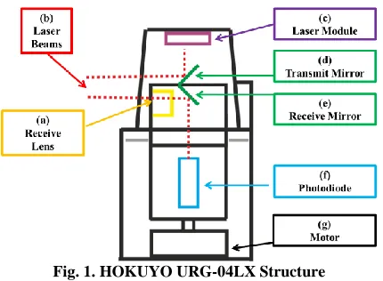
Developed specifically for robot platform navigation applications, the Hokuyo URG-04LX, features a 785nm Class 1 laser scanning a maximum 240° sweep angle, with an angular resolution of 360/1024° and a quoted maximum range of 4095 mm. Accuracy is quoted as ±10 mm at range distances of up to 1000 mm and rising to ±2% of the total distance for the remainder of the range scale. Two alternate modulation frequencies (46.55 and 53.2 MHz) are employed on transmitted light beams, while two ADCs sample the received optical beam for subsequent digital phase difference measurement [41]. A simplified scanner model is shown in Fig. 1. The infrared laser projects downward to an inclined mirror mounted on an optically encoded rotary stage, resulting in a horizontal output beam. The returning beam is focussed on another inclined mirror and converted to a vertical beam for reception on the horizontal faced photodiode. A brushless motor rotates the rotary stage, with position feedback provided by an optical encoder. An Application Specific Integrated Circuit (ASIC) features two ADC’s, motor position measurement control electronics and frequency specific clock and timing signals necessary for operation. RS232 and USB communication buses are available and offer the potential of real time data transmission and capture. A proprietary Hokuyo ASCII based communication protocol exists codenamed Scanning sensor Command Interface Protocol (SCIP) to allow

control of sensor operation and features such as resolution, sweep angle and operation.

Fig. 1. HOKUYO URG-04LX Structure

This sensor has been utilised on a variety of wheeled, crawler and aerial platforms [42-45]. The author, system developers, and adopters have both documented and experienced measurement errors when dealing with glossy reflective surfaces [14, 28, 41, 46, 47], due to the effects of specular reflection and saturation of the photodiode [41].

A. Reflected & Received Optical Beam

Accurate information and knowledge of surface condition and properties, prior to and during LRF scans is challenging. As the optical intensity of the transmitted laser remains approximately constant due to the fixed input power, the effect of Sensor to Surface Distance (SSD) and surface local conditions affect the intensity of the reflected laser beam. Therefore parameters of the received optical signal are a function of the local surface condition and can therefore be used to infer information regarding the surface.

Recent developments with respect to firmware and communication protocol (SCIP 2.0) have enabled operators of the Hokuyo URG-04LX to measure and monitor a number of additional received signal parameters such as the received optical intensity and gain controller values [48]. Received optical intensity is related to the reflected optical intensity after removing the effects of distance and inclination [47]. As discussed in [46], saturation of the Avalanche Photodiode (APD) during operation, particularly with highly glossy surfaces, requires use of an inbuilt Automatic Gain control Circuit (AGC). Only consistent or unmodified received signal intensity data permits discrimination of parameters related to the surface material. Work undertaken in [47] to establish the transfer function of the AGC determined the relationship was nonlinear with the original unmodified received optical luminous intensity (Restored Intensity) (Ir) given by Equation 2.

𝐼

=

𝑉𝑎 (2) Where:

Additionally, based on the measured Ir it is possible to record rejected or zero range data at a particular scan point due to excessively low or excessively high reflected light [33].

IV. EXPERIMENTAL MOTIVATION

Much of the previous work relating to the operation, use and characterisation of the Hokuyo URG-04LX and other similar laser range scanners, have focused on single beam analysis, on simple matt materials, where the remaining 2D sweep angle scanning potential is neglected [14, 33, 46]. This approach is limited in practice due to the potential large volume of data available when fully utilising a sweeping laser range scanner. Furthermore, considering the widespread industrial use of materials such as carbon and stainless steels, aluminium, concrete and plastics, all with widely varying surface reflectance characteristics, it is essential to further evaluate performance operating with such surfaces.

To fully characterise the LRF for industrial deployment it is clear that a full sweeping scan, with variation in material surfaces such as those found in a practical inspection scenario has to be considered. The materials considered, based on their use in industrial environments, were aluminium, carbon steel, stainless steel, portland cement concrete, plywood, polyvinyl chloride (PVC), Poly(methyl methacrylate) (PMMA) also known as acrylic glass or Perspex representing transparent surfaces such as windows and finally white paper symbolising matt surfaces such as plasterboard. Many typical industrial surfaces are of large area often consisting of multiple sheets of plate (2000 x 1000 mm) or mass poured concrete sections (> 5000 mm wide). Therefore a large as possible surface sweeping scan was desired to analyse the system performance. A sample area of 800 mm width was selected on the basis of being both acceptable in terms of size, while also being practically manageable. Due to the practicalities of undertaking a portland cement concrete inspection a pre-cast slab was selected with a limited sample surface width of 700mm. The selected samples are shown in Table 1.

Material Sample Surface

Description

Paper (PAP)

White coated woven paper Media Weight:120g/m2 Area Dimension: 900 x 600 mm Aluminum

(ALU)

Aluminum Sheet, Thickness Alloy:1050, Standard: EN 485 Area Dimension: 900 x 600 mm Carbon

Steel (ST)

Cold Reduced Steel Sheet Standard: BS EN 10131 Area Dimension: 900 x 600 mm

Stainless Steel (SS)

Cold Rolled Stainless Steel Sheet

Specification:1.4301 2B Standard: BSEN 10088-4 Area Dimension: 900 x 600 mm

Concrete (CON)

Standard Finish British Standard Paving Standard: BS EN 1339

Area Dimension: 700 x 600 mm PVC

(PVC)

Polyvinyl Chloride (PVC) Sheet,

Standard:ASTM-D-1784-99, Class 12454-B Area Dimension: 900 x 600 mm

Wood (WO)

Structural Hardwood Plywood Sheet, Standard:EN13986, BS EN 636-2, BS EN 314 Area Dimension: 900 x 600 mm

Perspex (PER)

Clear Cast Perspex Sheet Standard:ISO7823-1

Area Dimension: 900 x 600 mm

Table 1. Test Sample Surface Information Reference

Prior knowledge of typical pose variations and scanning limitations, when deploying mobile NDE inspection platforms [7, 49] defined the maximum angular deviation to be considered in each axis as ± 4°.

V. EXPERIMENTAL CONCEPT

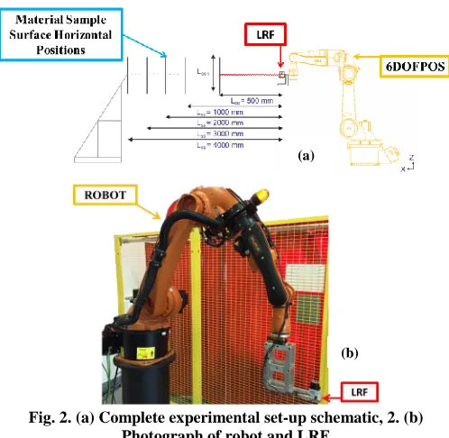
The LRF was mounted on the end of an industrial six Degree Of Freedom (D.O.F.) robot [50]. This approach allowed for controlled movement and repeatable scanning positions, not only in traditional 3 DOF (x,y,z) positions but also in roll (C), pitch (B) and yaw (A) orientation angles. The LRF pose was remotely controlled with custom code implemented through the KUKA Robot Sensor Interface [51], providing bi-directional pose information every 12 ms. Therefore the desired pose could be transmitted from a remote computer and the actual pose as measured from the internal encoders received by the external computer.

A manually operated linear rail allowed movement of the material sample along the X-axis direction of the robot with a maximum sensor to surface distance (SSD) of approximately 4 m, matching the specified detection range of the LRF. This is illustrated and shown below in Fig. 2.(a) with a close up photograph of the robot and LRF shown in Fig. 2.(b).

Fig. 2. (a) Complete experimental set-up schematic, 2. (b) Photograph of robot and LRF

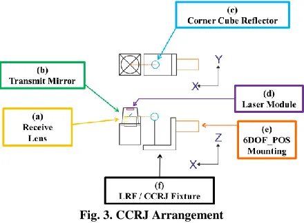
A metrology based Leica laser tracker [52] utilising an interferometer measurement system, which can measure the 3 DOF position of a retro reflector in free space to accuracies of ±0.2µm + 0.15µm/m, was used for measurement distance and alignment tasks. A Corner Cube Reflector Jig (CCRJ) was produced which when substituted with the LRF on the end of the robot, had its reflector centre vertical height matched to the midpoint height between the LRF transmit mirror and LRF receive lens. (Fig. 3). A simplification assumption was made that this point matched both the transmit and receive beam exit and entry point. This allowed the LRF position in free space to be estimated.

(a)

Fig. 3. CCRJ Arrangement

Five different SSD distances were investigated of nominal values 500, 1000, 2000, 3000, 4000 mm. These were selected to best represent the typical range of industrial stand-off distances compatible with the Hokuyo sensor.

The linear rail was aligned normal to the robot Y- axis along the full range, to ensure the sample remained parallel to the XY plane of the robot. Secondly, the SSD was measured accurately by direct measurement of 3 points on the sample surface, to give the surface plane and its normal distance between it and the nominal zero angle orientation pose of the CCRJ. The actual measured SSD were then obtained to be 532.0, 1020.4, 2001.1, 2993.9 and 3994.2 mm. These specific values were a limitation of the scanning rail. The home position of the robot was varied to account for any offset resulting from the thickness of the various samples. This process allows all measurement samples to be at accordingly similar SSD.

As the SSD increased and each sample scan area width remained constant, the scanning sweep angle was reduced to allow the LRF sweep to remain on the sample. The scan angles and corresponding number of sweep points were reduced as the SSD increased (Table 2).

SSD (mm)

Sweep Angle (°)

Potential Sweep Points

Actual Sweep Points

Sweep Angle (°)(Concrete)

Sweep Points (Concrete)

Actual Sweep Points (Concrete) 532.00 73.88 210.15 209 66.68 189.67 189 1020.44 42.80 121.76 121 37.86 107.69 107 2001.15 22.61 64.30 63 19.84 56.46 55 2993.93 15.22 43.29 43 13.34 37.93 37 3994.22 11.42 32.53 31 10.016 28.49 27

Table 2. LRF Scanning Parameters

The actual number of sweep points per distance was reduced to an odd number, to ensure there was a single normal beam with an even number of points both clockwise (right) and anti-clockwise (left) of it.

As discussed previously, the maximum angular deviation to be considered in each axis was ± 4°, with 2° increments giving therefore five distinct angular orientations per position. Furthermore each angle was varied systematically in turn so as to analyse the effects of rotation changes in all three axes independently.

When considering angle orientation (A, B & C) and the five possible values (-4°, -2°, 0°, 2° & 4°), a total of 125 discrete

measurement points are produced, spaced between 25 separate Cartesian (X,Y,Z) positions.

To ensure the LRF swept laser points remained within range on the sample surface, it was clear that any deviation in the yaw and pitch angles, required corrective deviations in the Y and Z axes respectively. This ensured that the central normal LRF beam remained positioned in the same point on the sample surface throughout all angular movements. Measurements undertaken at increased SSD therefore featured increased Y and Z travel of the LRF from the nominal centre to ensure the central perpendicular beam was reflected from the same point on the surface.

As the Hokuyo sensor can only output one measurement parameter (range, intensity or AGC) at a time, if it is desired to maintain the lowest minimum angular spacing, a number of measurements were undertaken at each discrete pose in a sequential fashion. Ten scans were undertaken of each parameter to evaluate noise and variation in the data measurement

After reviewing the separate modulation frequency received intensity (Io) and AGC values, and noting the minimal variation existing between each of the corresponding sets, a decision was taken to average both. Therefore the final measurement output at each pose location is summarised in Fig. 4:

Fig. 4. LRF Scanning Procedure

It must be noted that the LRF was operating for a minimum of 90 minutes prior to any measurement or scanning as recommended in [14, 28]. This reduced any potential drift effects present in the measurement data, due to an increase in internal operating temperature [28]. Additionally all measurement scans were undertaken in normal indoor laboratory ambient lighting conditions.

In order to evaluate the error in the range data captured by the LRF, this data firstly had to be transformed into a common global coordinate frame. The laser tracker provided the absolute ground truth positioning system and all measurements are with respect to the frame of reference of the laser tracker. The 3 D.O.F. Cartesian position of the CCRJ at the each of the 25 distinct measurement locations, where the five orientations angles are manipulated, were measured and recorded by the laser tracker. The remaining 3 D.O.F. orientation angles of the CCRJ were measured by the KUKA manipulator and then coordinate transformed, using a least squares fitting method, into the frame of reference of the laser tracker using the known 3 D.O.F. Cartesian position data [53]. A final coordinate transform was used to transform the LRF measurement data into the frame of reference of the laser tracker.

10x LRF range scans with corresponding scan angle & points for given SSD

10x Averaged received intensity scans with corresponding scan angle & points, for given SSD, across both modulation frequencies

10x Averaged AGC scans with corresponding scan angle & points, for given SSD, across both modulation frequencies

VI. LRF CHARACTERISATION AND PERFORMANCE VALIDATION

Given the large volume of measurement data recorded during the complete study, it is worth summarising that with each distinct material distance trial, 125 separate range scans, each nominally consisting of a minimum of 27 to a maximum of 209 distinct points, are measured along with their corresponding intensity and AGC values. Simple analysis of such data, bearing in mind the large number of varying parameters, is not easily practical and required some compromise to aid overall understating.

A. PMMA Perspex Surface Inspection

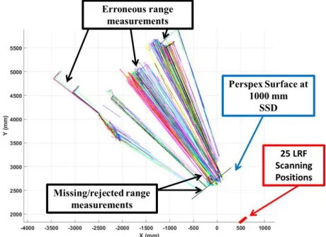
The high light transmission properties of the Perspex surface presented a highly challenging surface on which to perform optical based laser range scanning [54,55]. After reviewing the raw data, the authors are of the opinion that it was not suitable to perform credible error or accuracy characterisation on the material given the large scale and variation in range errors recorded. For reference, it was analysed that a minimum of 91.39% of the measured scan points, across all SSD’s, were classed as rejected by the LRF or outwith ±10% of the nominal SSD. The scan plan view for Perspex at SSD of 500 mm is shown below (Fig. 5), highlighting the raw range data and the clear large-scale errors recorded by the LRF.

Fig. 5. PMMA Perspex LRF Scan Plan View showing large quantity of missing and inaccurate range measurements data

B. Distance Error Quantification

Distance error was calculated for each individual scan point as the shortest perpendicular distance between the point and the sample surface. This was achieved by projecting each scan point into the global 3D world coordinate system. Therefore for each scan, a number of error measurements were recorded corresponding to the number of individual scan points specified in the acquisition. The Root Mean Square Error (RMSE) of the LRF distance error with respect to each material surface was computed to generate a single error.

Across all samples, it was consistently found that RMSE mean error increased nonlinearly with increased yaw and pitch angles, with negligible effect from roll rotation. Therefore, in order to simplify the analysis and presentation of the data, the

yaw and pitch angles were combined to form a single angle. This single value is computed and represented by the angle between the normal of the material plane and the roll axis of the LRF. As such, 5 RMSE measurements were computed at each position. For illustrative purposes, the mean RMSE value, plotted against the corresponding combined angle, is shown for both paper and aluminum at a nominal SSD in Figs. 6. Due to the symmetry of the orientation sweep pattern, where the unique values were 5.65 ̊, 4.47 ̊, 4.00 ̊, 2.83 ̊, 2.00 ̊, 0 ̊ , multiple mean RMSE values map to the same combined angle with the exception of the zero angle. The RMSE mean and standard deviation for each material and SSD is tabulated in Table 3. For brevity, the maximum error at each SSD is highlighted in bold and correspondingly the lowest in italics.

Fig. 6. (a) AB Angle LRF RMSE Mean Error Nominal SSD 4000 mm (Paper), 5. (b) AB Angle LRF RMSE Mean Error Nominal

SSD 4000 mm (Aluminium)

Property Nominal

SSD (mm) PAP ALL ST SS CON PVC WO

RMSE Mean (mm)

500 35.25 77.67 55.47 37.37 20.8 31.96 57.13

1000 50.21 46.72 33.82 42.78 55.98 30.82 70.91

2000 48.80 76.09 26.00 89.82 65.28 76.62 83.18

3000 69.70 48.57 48.17 94.92 88.00 100.12 95.99

4000 68.02 49.67 50.72 94.04 90.73 76.67 99.32

Distance Error (Combined

Angle) Standard Deviation (mm)

500 1.50 2.44 0.82 0.75 1.60 1.83 1.26

1000 3.87 6.74 2.48 2.26 11.12 2.91 2.31

2000 6.20 11.2 5.29 4.93 7.92 6.75 4.67

3000 9.22 8.72 9.74 9.44 7.60 8.11 11.05

4000 11.62 16.39 13.35 11.06 15.22 14.8 11.38

Table 3. Distance error quantification for all materials at varying SSD, with varying pose orientation angle

When considering RMSE Mean error it is clear that not only considerable magnitude error exists across all materials, ranging from a minimum of 20.8 mm to a maximum of 100.12 mm. For reference, the minimum RMSE mean error measured across the Perspex surface was evaluated to be 499.77 mm at a nominal SSD of 3000 mm. Additionally, distinct variation exists when considering each separate material and the general trend of these errors with respect to increasing SSD. Across all samples, it was consistently found that RMSE mean error increased with increased orientation angle from the zero value, with a nonlinear trend beginning to be discernible with combined angle orientation. Additionally, it was clear that increased nonlinearity was evident at increased SSD. Furthermore, when considering RMSE mean error no nonlinear effects were witnessed when considering increased roll angle rotation. It is clear that the standard deviation of the distance error increased with increasing SSD.

C. Overall Distance Error Quantification

To simply highlight the magnitude and polarity of the distance error of all scans across the complete angular

orientation window, a normal distribution histogram was introduced to represent and encompass the range distance from the LRF to each individual scan point in the complete measurement scan. This was plotted against the true SSD as measured by the laser tracker.

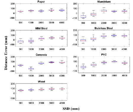
The magnitude and polarity of the distance error of all scanned points across the complete angular orientation window was evaluated for each material at the five distinct SSD’s. Figure 7 highlights mean, maximum, minimum and 5/95% Interquartile Range (IQR) error in typical boxplot fashion

Fig. 7. Magnitude and polarity of distance errors across all sample surfaces. It should be noted that SSD (mm) corresponds to the X-Axis of all subplots and correspondingly Distance Error

(mm) to the Y-Axis.

While for matt surfaces such as paper and wood the error always remained positive, it can be seen that all three metallic surfaces and PVC they exhibit a change of polarity from negative to positive from nominal SSD of 500 to 2000 mm. Additionally, as can be seen, all three metallic surfaces exhibit a larger IQR, which nominally reduces with distance.

D. Restored Intensity Quantification

Using Equation 2the restored intensity for each scan across the whole scanning window can be calculated. Calculation of the area under this curve yields a single value to describe the intensity of the reflected scan. Similarly to the above distance error, the Restored Intensity Area mean and standard deviation were computed from the data measured at each combined angle and are highlighted in Table 4. Again, the maximum value at each SSD is highlighted in bold and correspondingly the lowest in italics. As noted in [47] Restored Intensity is a unitless quantity and hence quantities in the following table are unitless.

Property Nominal

SSD (mm)

PAP ALL ST SS CON PVC WO

Restored Intensity Area Mean

500 54242.80 21711.60 33386.10 33313.70 43928.30 40537.00 53777.70 1000 28571.00 13152.60 19118.80 18262.50 35525.50 17990.60 28556.50 2000 13292.80 7005.02 7650.40 8230.51 7214.63 5973.49 13463.40

3000 6015.19 5148.29 3114.57 4469.79 2339.84 2289.70 6258.85

4000 2531.76 3948.78 1456.78 2722.75 1068.24 1118.19 2324.02 Restored

Intensity Area (Combined

Angle) Standard Deviation

500 52.45 674.53 235.28 309.88 80.58 348.92 352.39

1000 46.88 885.58 357.68 240.53 339.05 409.25 270.43

2000 52.78 977.18 579.15 281.82 338.96 577.54 243.44

3000 50.05 901.62 520.29 259.41 153.12 349.64 427.11

4000 32.26 1061.31 280.03 606.8 84.46 204.11 182.23

Table 4. Restored Intensity quantification for all materials at varying SSD, with varying pose orientation angle

As can be seen by comparison of Tables 3 & 4, no direct correlation exists between mean RMSE and the restored intensity area mean. What is clear from Table 4 is that the lowest overall intensity standard deviation return was always from the paper surface, while generally the highest was from the aluminum. Again it was generally found that Restored Intensity Area Mean increased with increased orientation angle from the zero value, with a nonlinear trend beginning to be discernible when considering increased combined orientation angle. While generally similar with regards to increased nonlinearity being evident at increased SSD, those materials with larger standard deviations feature a pronounced variability in nonlinearity. Again, when considering Restored Intensity Area Mean, no nonlinear effects were evident when considering increased roll angle rotations.

E. Scan Point Rejection Quantification

As discussed above, rejected measurement points, based on low or high reflected intensity error codes, are logged at any particular scan point and hence complete scan window. Additionally for the purposes of this study points outwith ±10 % of the nominal SSD were also classed as rejected, based on overall desired acceptable performance level. Therefore the percentage of rejected points per scan window was calculated. The overall percentage rejection mean and standard deviation, as a function of combined angle, is documented in table below Table 5. Again, the maximum value at each SSD is highlighted in bold and correspondingly the lowest in italics. NPR denotes No Points Rejected in the scan.

Property Nominal

SSD (mm) PAP ALL ST SS CON PVC WO

Percentage Rejections Mean

500 NPR 34.32 30.47 NPR NPR NPR NPR

1000 NPR 5.11 NPR NPR NPR NPR NPR

2000 NPR 10.46 NPR NPR NPR NPR NPR

3000 NPR 55.85 6.55 28.50 NPR 23.91 NPR

4000 NPR 65.99 28.33 42.10 6.59 49.84 NPR

Percentage Rejections (Combined Angle) Standard Deviation

500 N/A 2.95 3.32 N/A N/A N/A N/A

1000 N/A 6.65 N/A N/A N/A N/A N/A

2000 N/A 8.18 N/A N/A N/A N/A N/A

3000 N/A 17.46 8.55 15.05 N/A 18.07 N/A

4000 N/A 21.51 15.99 20.25 11.04 20.52 N/A

Table 5. Rejected measurement point quantification for all materials at varying SSD, with varying pose orientation angle

metallic surfaces, concrete and PVC feature rejections at higher SSD. Steel surfaces document both high percentage rejection and corresponding standard deviations particularly at the lowest SSD.

F. Measurement Rejection Prediction

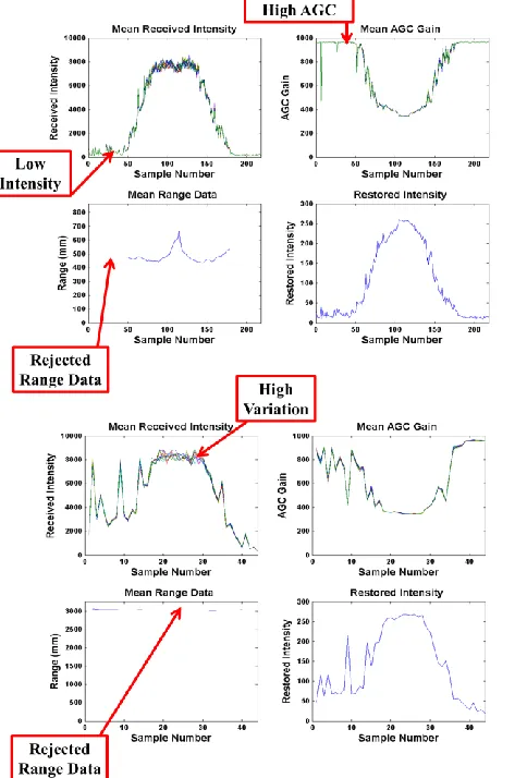
From study of measured parameters, range, received intensity and AGC, it became clear from observation, that large variation in received intensity between each subsequent scan corresponds to measurement points which are rejected as they fall out with a specified tolerance (±10 % of SSD ) and do not produce a corresponding intensity based error code.

Low received intensity values presented problems for the sensor and often resulted in rejected range data, with corresponding high AGC gain, shown in Fig. 8.(a). These low intensity values produced a corresponding error code however no specific value was identified to a represent a low received intensity error. Similarly received intensity data greater than the high intensity threshold (Fig. 8(b)) often produced erroneous range data but did not always produce the according error message.

Fig. 8 Aluminium Sheet LRF Rejected Range Data Points a) Nominal 500 mm SSD, b) Nominal 3000 mm SSD

To evaluate the probability of bad or rejected measurement data based on restored intensity variation, the following procedures were undertaken. The standard deviation of restored intensity data from each of the individual ten mean

values sampled at each pose was calculated. Concurrently the range data from each corresponding sample point was classified as a valid or rejected point. Therefore the validity of all measurement points across a full scan can be plotted against the restored intensity standard deviation.

The data was further divided by binning all data within bins of incremental width of standard deviation 10, chosen based on a compromise of resolution and knowledge of the full scale range. Across each bin the validity of range measurement, in a range of zero to one, is calculated by:

𝑉𝑀𝑃 =_{𝑁𝑉𝑃+𝑁𝑅𝑃} 𝑁𝑉𝑃 (3)

Where:

VMP-Valid Measurement Probability, NVP -Number of Valid Measured Points and NRP-Number of Rejected Measured Points

Therefore within each bin a validity measurement probability value was calculated and could then be plotted accordingly for the whole range (Fig. 9) and documented in Table 6. The lowest VMP mean, standard deviation and maximum recorded standard deviation at each SSD is highlighted in bold. Again, aluminum features the greatest decrease in VMP with a corresponding increase in VMP standard deviation. Additionally, what is clear is the correlation between higher restored intensity standard deviation and rejected measurements and hence lower VMP.

Fig. 9. LRF Range Validity as a function of Restored Intensity Standard Deviation Nominal SSD 4000 mm (Aluminium)

Property Nominal

SSD PAP ALL ST SS CON PVC WO

VMP (Mean)

500 1 0.92 0.80 1 1 1 1 1000 1 0.99 1 1 1 1 0.98

2000 1 0.99 1 1 1 1 1

3000 1 0.304 1 0.40 1 1 1 4000 1 0.31 1 0.42 1 0.96 1

VMP Standard Deviation

500 0 0.24 0.19 0 0 0 0

1000 0 0 0 0 0 0 0

2000 0 0 0 0 0 0 0

3000 0 0.36 0 0.41 0 0 0 4000 0 0.34 2 0.40 0 0 0

Max Received Intensity Standard Deviation

500 371 1371 421 1211 351 401 361

1000 441 1721 411 401 1061 401 381

2000 361 1461 341 351 181 221 331

3000 171 451 271 371 91 131 221

4000 101 431 151 381 91 81 111

Table 6. Received Intensity Performance Metrics

G. Range Data Stability

pose is shown below for each material in Table 7. Again, Aluminium exhibits the largest variance from mean in individual range measurements.

Property SSD

(mm) PAP ALL ST SS CON PVC WO

Histogram Sigma (mm)

500 2.75 3.56 2.76 2.97 2.69 2.54 2.48

1000 3.23 9.41 3.08 3.23 12.88 3.07 3.40

2000 2.50 4.00 2.62 3.73 2.51 2.72 2.73

3000 2.48 4.25 3.23 3.20 2.35 3.78 2.29

4000 2.66 4.72 3.92 3.71 3.62 6.63 2.57

Table 7. Standard Deviation of range data, at normal 0, 0, 0 orientation

VII. LRF SURFACE IDENTIFICATION

For the surfaces sampled in this study, it was proposed that it was possible to identify the surface being scanned based on the parameters evaluated above. In turn, determination of the surface allow correction factors to be applied to improve the LRF performance

As found above and in [42] and through observation of the measured datasets, there existed a relationship between the optical luminous intensity (Ir), across the swept angle range, and the sample surface. Therefore through analysis of the restored intensity a broad appreciation of the sample surface can be determined [56-58]. It is worth noting that for the purposes of this study the overall sample surface parameter being identified, consists of the combined effect of surface gloss, surface texture, often defined by surface roughness, and surface colour [59]. Given the variation in each of these parameters, especially surface colour, across the seven materials sampled, a valid assumption and approximation can be made that basic material identification can be therefore achieved. For simplicity and an initial undertaking, only the zero orientation datasets (A=B=C=0°) were considered. A polynomial was selected to best fit all restored intensity curves for every material at each SSD. Through inspection of the data it was established a fifth order polynomial sufficiently captured the overall curve trends.

Discrimination and therefore identification of the surface based on the restored intensity of the LRF was deemed feasible, due to the variation in coefficient values with each material. For classification to occur similar coefficients are computed for a scanned surface received intensity profile. These coefficients are subsequently compared on a per-coefficient basis, in terms of Euclidean distance, to the coefficients previously computed for each material. The surface classification is achieved through that with the greatest consensus in terms of total minimum Euclidean distance.

An assumption was therefore made that the scanned environment could be viewed to be composed of linear segments located to and scanned perpendicularly by the LRF. This was deemed suitably valid for many large industrial scanning scenarios, particularly when mainly considering large surfaces such as walls and roofs.

VIII. LRF RANGE CALIBRATION

With knowledge of the material, it is then conceivable that correction factors can be applied to calibrate the LRF for range accuracy, when scanning challenging surfaces. This is a further development of the material agnostic calibration

methods presented previously [14, 33, 46, 60, 61]. Such strategies could be established using reference calibration data acquired in a similar manner to the above body of work, across many sample surfaces and ranges, while estimating correction parameters related to correction factors based on material surface, range and sweep angle point. Such a technique would ultimately establish calibration factors for each scan point, which could then be applied to future measured points based on the current estimation of material surface identification and range. Such a procedure was established for the Hokuyo LRF to correct for the errors identified and documented previously. The calibration procedure accounts and compensates for artefacts and errors documented previously when scanning common industrial surface materials. Again the assumption was made that the scanned environment could be viewed to be composed of linear segments between scanned points, which again is normally valid for many large industrial scanning scenarios. Only range data acquired perpendicular to the material surface, (A=B=C=0°) collected during the sensor characterisation phase was utilised. This simplification was introduced for practical and computational reasons.

Using the range data previously acquired at each of the five specific SSD distances, for each material, a curve fitting procedure (fifth order Gaussian) was applied to the range data. A Gaussian based fitting approximation curve was chosen on the basis of suitability, with respect to lowest fitting error. The resultant range scale mapping of the fitted curve to the true range measured by the LAT was determined at each distinct scan point. Following this procedure, a correction curve corresponding to each LAT measured SSD, for each material, was generated. This allowed a resultant correction curve, per scan point and material, to be stored for further operations.

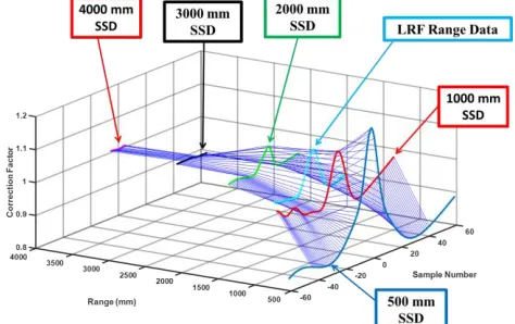
Correction curves for true distances lying between those recorded using the laser tracker were obtained via linear interpolation, for simplicity, between each of the five distinct laser tracker measured SSD distances. During online operation, the mean range of the received range measurement was computed. This distance was used to generate the corresponding correction curve, located on a point between the five nominal SSD distances (Fig. 10.). This is an obvious approximation as the true range distance may not correspond to the mean range. This assumption was made due to the calibration algorithm requiring a range measurement estimation.

The corresponding correction scaling factor per scan point, based on the acquired mean range data, can then be applied to the received range measurement data to correct for and reduce the overall distance error.

The calibration and correction procedure was then applied to the previously acquired datasets, with different SSDs and materials. The RMSE across the complete scan window at each nominal SSD, for the zero orientation angle pose, for each material is recorded in Table 8. (Uncorrected -U) and (Corrected -C). Highlighted is the overall reduction in RMSE with the corrected calibration procedure.

Nominal SSD (mm)

RMSE (mm) Material

Paper Aluminum Steel Stainless

Steel Concrete PVC Wood

U C U C U C U C U C U C U C

500 45.34 12.17 XOB XOB XOB XOB 37.92 9.93 26.00 11.79 23.65 11.69 68.36 14.13

1000 53.42 7.64 49.98 19.16 25.91 24.20 50.91 6.29 50.68 12.40 37.05 5.96 74.39 8.73 2000 41.77 5.93 84.95 6.69 22.86 7.09 91.26 6.39 50.60 1.65 72.34 6.74 79.11 5.46 3000 62.32 5.78 XNVD XNVD 35.58 3.89 83.21 7.59 76.53 2.87 86.22 5.89 83.78 5.48

4000 XOB XOB XOB XOB XOB XOB XOB XOB XOB XOB XOB XOB XOB XOB

Table 8. Uncorrected & Corrected LRF Range RMSE

Where XOB is defined as a dataset where mean range

measurement is out with the minimum (532.00) and maximum (3994.22) SSD distance, yielding the correction inoperable. Similarly, XNVD is defined as a dataset which contains no valid

data to perform a corresponding scaling correction factor. This was found to occur when high intensity points, with corresponding error code, were detected and constitute the complete correction window allowing no scaling correction data to be generated.

A. Industrial Sample Range Scanning Correction

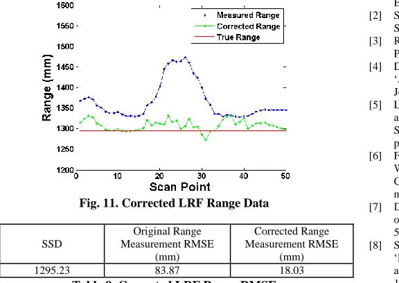
To highlight successful proof of principal a separate test sample was scanned and measured to ascertain the calibration correction algorithm performance. The aluminum sample surface was scanned at a laser tracker measured SSD of 1295.23 mm. After correct classification of surface material, the correction algorithm was applied and its result is shown in Fig. 11. RMSE of the original and corrected range measurement data is shown in Table 9.

Fig. 11. Corrected LRF Range Data

SSD

Original Range Measurement RMSE

(mm)

Corrected Range Measurement RMSE

(mm)

1295.23 83.87 18.03

Table 9. Corrected LRF Range RMSE

As shown by Fig. 9. and the reduced RMSE (Table 9.), such an approach further improves the performance and accuracy of the optical based LRF sensor. This has clear benefits to any automated NDE system, deploying such an LRF for pose estimation, albeit based on a priori calibration data.

IX. LRF SURFACE SCANNING, MATERIAL IDENTIFICATION AND CALIBRATION CONCLUSION

A thorough study of the performance of the Hokuyo URG-04LX and characterisation of the system when scanning various commonly found industrial materials was undertaken. Specifically, the study investigated the effects of small orientation angle changes of the LRF, in a similar manner to which it would experience when being deployed on a mobile robotic platform. A detailed process of error measurement and visualisation was undertaken on a number of parameters, not limited to traditional range data but also received intensity and AGC gain. This work highlights that significant range distance errors are introduced when optically laser scanning common industrial materials. The specular reflective nature of some materials, such as aluminum, stainless steel and PVC, results in large deviation in range data from the true value, with mean RMSE errors as high as 100.12 mm recorded.

A detailed procedure for evaluating the performance of other laser range sensors, while operating under similar industrial conditions has been established, encompassing parameters such as sensor orientation angle, surface material and reflectivity.

Furthermore, a novel computationally inexpensive algorithm for range correction in industrial scenario was proposed and developed. The correction algorithm was shown to reduce the RMSE error associated with range estimation on a planar aluminium surface from 6.48% to 1.39% of the measured SSD. This new research approach will be further developed to handle incidence angles other than normal and greater material combinations, to allow future industrial deployment.

REFERENCES

[1] HSE ‘The Health and Safety of Great Britain’ Health and Safety Executive 2009, http://www.hse.gov.uk/, Accessed Apr. 2014.

[2] SEPA ‘Protecting Scotland’s Environment – A 10 Year Perspective’ Scottish Environmental Protection Agency, 2011.

[3] Ramírez, P. A. P. and Utne, I. B. ‘Challenges due to aging plants’, Process Safety Progress, vol. 30, issue 2, pp. 196–199, 2011.

[4] Dobie, G., Summan, R., Pierce, S. G., Galbraith, W. and Hayward, G., ‘A noncontact ultrasonic platform for structural inspection’ Sensors Journal, IEEE , vol.11, no.10, pp. 2458-2468, Oct. 2011.

[5] Lim, R.S.; Hung Manh La; Weihua Sheng, "A Robotic Crack Inspection and Mapping System for Bridge Deck Maintenance," Automation Science and Engineering, IEEE Transactions on , vol.11, no.2, pp.367,378, April 2014

[6] Friedrich, M., Dobie, G., Chan, C.C., Pierce, S.G., Galbraith, Marshall, W. S., and Hayward, G., ‘Miniature Mobile Sensor Platforms for Condition Monitoring of Structures’. Sensors Journal, IEEE , vol.9, no.11, pp.1439-1448, Nov. 2009.

[7] Dobie, G., Summan, R., MacLeod, C.N. and Pierce, S.G., ‘Visual odometry and image mosaicing for NDE’. NDT and E International, vol. 57, pp. 17-25, 2013

[9] C. N. Macleod, S. G. Pierce, J. C. Sullivan, A. G. Pipe, G. Dobie and R. Summan, "Active Whisking-Based Remotely Deployable NDE Sensor," in IEEE Sensors Journal, vol. 13, no. 11, pp. 4320-4328, Nov. 2013. [10] Dobie, G., Spencer, A., Burnham, K., Pierce, S. G., Worden, K.,

Galbraith, W. and Hayward, G. ‘Simulation of ultrasonic lamb wave generation, propagation and detection for an air coupled robotic scanner’, Ultrasonics, vol. 51, issue 3, pp. 258-269, 2011.

[11] Morrison, J. P., Dixon, S. M., Potter, D. G. and Jian, X., ‘Lift-off compensation for improved accuracy in ultrasonic lamb wave velocity measurements using electromagnetic acoustic transducers (EMATs)’, Ultrasonics, vol. 44, pp. 1401–1404, Dec. 2006.

[12] Huang, S., Zhao, W., Zhang, Y. and Wang, S., ‘Study on the liftoff effect of EMAT’, Sens. Actuators A, Phys., vol. 153, no. 2, pp. 218–221, Aug. 2009.

[13] Lee, J. Y., Hwang, J. S., Lee, K. E. and Choi, S. H. ‘A Study of leakage magnetic flux detector using hall sensors array’, Key Eng. Mater., vols. 306–308, pp. 235–240, Mar. 2006.

[14] Kneip, L., Tache, F., Caprari, G. and Siegwart, R., ‘Characterization of the compact Hokuyo URG-04LX 2D laser range scanner’, Robotics and Automation, ICRA '09. IEEE International Conference on , pp.1447-1454, May 2009.

[15] Iborra, A., Pastor, J.A., Alvarez, B., Fernandez, E. and Merono, J.M.F., ‘Robots in radioactive environments’, Robotics & Automation Magazine, IEEE , vol.10, no.4, pp.12-22, Dec. 2003.

[16] Hebert, M., ‘Active and passive range sensing for robotics’, Robotics and Automation, Proceedings. ICRA '00. IEEE International Conference on , vol.1, pp.102-110 vol.1, 2000.

[17] Curtis, P. and Payeur, P., ‘An integrated robotic laser range sensing system for automatic mapping of wide workspaces’, Electrical and Computer Engineering, Canadian Conference on, vol.2, pp.1135-1138, May 2004.

[18] Curtis, P., Yang, E.S. and Payeur, P., ‘An Integrated Robotic Multi-Modal Range Sensing System’, Instrumentation and Measurement Technology Conference, IMTC, Proceedings of the IEEE , vol.3, pp.1991-1996, May 2005.

[19] Thrun, S., Burgard, W. and Fox., D., Probabilistic Robotics. MIT Press, Cambridge, MA, 2005.

[20] Hua, H., Wang, Y. and Yan, D., ‘A low-cost dynamic range-finding device based on amplitude-modulated continuous ultrasonic wave’, Instrumentation and Measurement, IEEE Transactions on, vol. 51, no. 2, pp. 362-367, Apr. 2002.

[21] Loianno, G., Lippiello, V. and Siciliano, B., ‘Fast localization and 3D mapping using an RGB-D sensor’, Advanced Robotics (ICAR), 16th International Conference on, pp. 1-6, Nov. 2013.

[22] Souza, A.A.S. and Maia, R.S., ‘Occupancy-Elevation Grid Mapping from Stereo Vision’, Robotics Symposium and Competition (LARS/LARC), Latin American, pp. 49-54, Oct. 2013.

[23] Smith, P.W., Nandhakumar, N. and Chien, C.-H., ‘Object motion and structure recovery for robotic vision using scanning laser range sensors’, Robotics and Automation, IEEE Transactions on, vol. 13, no. 1, pp. 74-80, Feb. 1997.

[24] F. Santoso, M. A. Garratt, M. R. Pickering and M. Asikuzzaman, "3D Mapping for Visualization of Rigid Structures: A Review and Comparative Study," in IEEE Sensors Journal, vol. 16, no. 6, pp. 1484-1507, March15, 2016.

[25] Z. J. Diggins et al., "Range-Finding Sensor Degradation in Gamma Radiation Environments," in IEEE Sensors Journal, vol. 15, no. 3, pp. 1864-1871, March 2015.

[26] Chen, Y. D. and Ni, J., ‘Dynamic calibration and compensation of a 3D laser radar scanning system’, Robotics and Automation, IEEE Transactions on, vol. 9, no. 3, pp. 318-323, Jun. 1993.

[27] Adams, M.D., ‘Lidar design, use, and calibration concepts for correct environmental detection’, Robotics and Automation, IEEE Transactions on, vol.16, no.6, pp.753-761, Dec. 2000.

[28] Okubo Y., Ye E. and Borenstein J., ‘Characterization of the Hokuyo URG-04LX laser rangefinder for mobile robot obstacle negotiation’, Proc. SPIE 7332, Unmanned Systems Technology XI, Apr. 2009. [29] Kogut, G., Ahuja, G., Sights, B., Pacis, E.B. and Everett, H.R., ‘Sensor

Fusion for Intelligent Behaviour on Small Unmanned Ground Vehicles’, Proc. SPIE 6561, Unmanned Systems Technology IX, 65611V, May 2007.

[30] Chang, Y., Kuwabara, H. and Yamamoto, Y., ‘Novel Application of a Laser Range Finder with Vision System for Wheeled Mobile Robot’, ProE. of IEEE/ASME Int. Conf. on Advanced Intelligent Mechatronics, pp. 280-285, 2008.

[31] Zeng, S. and Weng, J., ‘Online-learning and Attention-based Approach to Obstacle Avoidance Using a Range Finder’, Journal of Intelligent Robot System 50, pp. 219-239, 2007.

[32] Choi, Y., Hong, J. and Park, K., ‘Obstacle Avoidance using Active Window and Flexible Vector Field with a Laser Range Finder’, Int. Conf. on Control, Automation and Systems, pp. 2123-2128, 2007. [33] Ye, E. and Borenstein, J., ‘A New Terrain Mapping Method for Mobile

Robots Obstacle Negotiation’, Proc. SPIE 5083, Unmanned Ground Vehicle Technology V, Sept. 2003.

[34] Ueda, T., Kawata, H., Tomizawa, T., Ohya, A. and Yuta, S., ‘Mobile SOKUKI Sensor System: Accurate Range Data Mapping System with Sensor Motion’, Int. Conf. on Autonomous Robots and Agents, pp. 309-314, 2006.

[35] Sohn, H. and Kim, B., ‘A Robust Localization Algorithm for Mobile Robots with Laser Range Finders’, ProE. IEEE Int. Conf. on Robotics and Automation, pp. 3545-3550, 2005.

[36] Lingemann, K., Nüchter, A., Hertzberg, J., Surmann, H., ‘High-speed laser localization for mobile robots’, Robotics and Autonomous Systems, vol. 51, issue 4, pp. 275-296, June 2005.

[37] Borges, G. and Aldon, M., ‘Line Extraction in 2D Range Images for Mobile Robotics’, Journal of Intelligent and Robotic Systems, vol. 40, issue 3. pp. 267-297, 2004.

[38] Nguyen, V.; Martinelli, A.; Tomatis, N. and Siegwart, R., ‘A comparison of line extraction algorithms using 2D laser rangefinder for indoor mobile robotics’, Intelligent Robots and Systems, IROS, IEEE/RSJ International Conference on , pp.1929-1934, Aug. 2005. [39] M. Dekan, F. Duchoň, A. Babinec, P. Hubinský, M. Kajan and M.

Szabová, "Versatile Approach to Probabilistic Modeling of Hokuyo UTM-30LX," in IEEE Sensors Journal, vol. 16, no. 6, pp. 1814-1828, March15, 2016.

[40] Koskinen, M., Kostamovaara, J. T. and Myllylae R.A., ‘Comparison of continuous-wave and pulsed time-of-flight laser range-finding techniques’, Proc. SPIE 1614, Optics, Illumination, and Image Sensing for Machine Vision VI, Mar. 1992.

[41] Kawata H., Ohya A., Yuta S., Santosh W. and Mori T., ‘Development of ultra-small lightweight optical range sensor system’, ProE. IEEE/RSJ Int. Conf. on Intelligent Robots and Systems, Edmonton, pp. 1078-1083, 2005.

[42] Łabęcki, P., Nowicki, M. and Skrzypczyński, P., ‘Characterization of a compact laser scanner as a sensor for legged mobile robots’, Management and Production Engineering Review, vol. 3, issue 3, pp. 45–52, Oct.2012.

[43] Winkvist, S., Rushforth, E. and Young, K.. ‘Towards an autonomous indoor aerial inspection vehicle’, Industrial Robot: An International Journal, vol. 40 issue 3, pp.196- 207, 2013.

[44] Pouliot, N., Richard, P. and Montambault, S., ‘LineScout power line robot: Characterization of a UTM-30LX LIDAR system for obstacle detection’, Intelligent Robots and Systems (IROS), IEEE/RSJ International Conference on, pp.4327-4334, Oct. 2012.

[45] Luo, R.E. and Lai C. C., ‘Indoor mobile robot localization using probabilistic multi-sensor fusion’, Advanced Robotics and Its Social Impacts, ARSO, IEEE Workshop on, pp. 1-6, Dec. 2007.

[46] Park, C.H., Kim D., You, B.J. and Oh, S.O, ‘Characterization of the Hokuyo UBG-04LX-F01 2D laser rangefinder’, RO-MAN, IEEE , pp. 385-390, Sept. 2010.

[47] Kawata, H., Miyachi, K., Hara, Y., Ohya, A. and Yuta, S., ‘A method for estimation of lightness of objects with intensity data from SOKUIKI sensor’, Multisensor Fusion and Integration for Intelligent Systems, MFI, IEEE International Conference on, pp. 661-664, Aug. 2008. [48]

http://www.hokuyo-aut.jp/02sensor/07scanner/download/data/URG_SCoku20.pdf Accessed Apr. 2014.

[49] MacLeod, C.N., Pierce, S.G., Summan, R., Dobie, G., Sullivan, J. C., Pipe, A. and Cao, J., ‘Remotely deployable aerial inspection using tactile sensors’, 40th Annual Review of Progress in Quantitative Nondestructive Evaluation, pp. 1873-1880, Baltimore, Maryland, USA, 2013

[50] KUKA KR5 ARC HW, http://www.kukarobotics.com, Accessed 04/2014.

[51] http://www.kuka-robotics.com, Accessed Apr. 2014.. [52]

http://www.hexagonmetrology.co.uk/leica-absolute-tracker-at901_283.htm, Accessed Apr. 2014..

[54] S. W. Yang and C. C. Wang, "On Solving Mirror Reflection in LIDAR Sensing," in IEEE/ASME Transactions on Mechatronics, vol. 16, no. 2, pp. 255-265, April 2011.

[55] X. Chen, D.Wang, and H. Li, “A hybrid method of reconstructing 3D airfoil profile from incomplete and corrupted optical scans,” Int. J. Mechatron. Manuf. Syst., vol. 2, no. 1/2, pp. 39–57, 2009

[56] Kirchner, N., Dikai Liu and Dissanayake, G., ‘Surface Type Classification With a Laser Range Finder’, Sensors Journal, IEEE , vol. 9, no. 9, pp. 1160-1168, Sept. 2009.

[57] Kirchner , N., Taha, T., Liu, D. and Paul, G., ‘Simultaneous material type classification and mapping data acquisition using a laser range finder’, Proc. Int. Conf. on Intelligence Technologies: Intelligent Technology in Robotics and Automation, 2007.

[58] J. Hancock, Laser intensity-based obstacle detection and tracking, Doctoral Dissertation, 1999.

[59] Sanmartín, P., Silva, B., and Prieto, B., ‘Effect of Surface Finish on Roughness, Color, and Gloss of Ornamental Granites’, J. Mater. Civ. Eng., vol. 23, issue 8, pp. 1239-1248, 2011.

[60] Kurisu, M., Muroi, H. and Yokokohji, Y., ‘Calibration of laser range finder with a genetic algorithm’, Intelligent Robots and Systems, IROS, IEEE/RSJ International Conference on, pp.346-351, 2007.