Identification of monetary policy in SVAR models: A data-oriented perspective

City, University of London Institutional Repository

Citation

: Fragetta, M. and Melina, G. (2013). Identification of monetary policy in SVAR

This is the unspecified version of the paper.

This version of the publication may differ from the final published

version.

Permanent repository link:

Link to published version

: http://dx.doi.org/10.1007/s00181-012-0632-y

Copyright and reuse:

City Research Online aims to make research

outputs of City, University of London available to a wider audience.

Copyright and Moral Rights remain with the author(s) and/or copyright

holders. URLs from City Research Online may be freely distributed and

linked to.

City Research Online: http://openaccess.city.ac.uk/ [email protected]

Identification of Monetary Policy in SVAR Models: A

Data-Oriented Perspective

Matteo Fragettaa _{and Giovanni Melina}∗b,c a_{University of Salerno, Italy}

b_{Birkbeck, University of London, UK} c_{University of Surrey, UK}

First version: 29th September 2011 This version: 9th May 2012

Abstract

In the literature using short-run timing restrictions to identify monetary policy shocks in vector-autoregressions (VAR) there is a debate on whether (i) contemporaneous real activity and prices or (ii) only data typically observed with high frequency should be as-sumed to be in the information set of the central bank when the interest rate decision is taken. This paper applies graphical modelling theory, a data-based tool, in a small-scale VAR of the US economy to shed light on this issue. Results corroborate the second type of assumption.

Keywords: Monetary policy; SVAR; Graphical modelling.

JEL Codes: E43; E52.

∗_{Corresponding author. Tel: +44 (0) 1483 689924; Fax: +44 (0) 1483 689 548.}

1

Introduction

Vector-autoregressions (VARs) are a widely used tool to provide stylized facts about responses of macroeconomic variables to structural shocks. These facts are usefulper se and also serve as guidelines in evaluating or calibrating theoretical business cycle models. The literature employing VARs to identify and estimate the effects of monetary policy shocks using short-run timing restrictions tipically distinguish among three sets of variables: (i) the information set, i.e. the set of variables known to the monetary authorities when the policy decision is taken; (ii) the policy instrument; (iii) the set of variables the value of which is known only after the policy is set. Such a distinction often suggests a block-recursive structure exploitable in identifying the VAR. Most of the existing empirical papers in the field can be classified into two broad groups, which differ in the content of the information set of the monetary authority. The first group of papers, that can be thought of following a “workhorse” approach, include, among many others, Christiano and Eichenbaum (1992), Christiano et al. (1996) as well as the influential paper by Christiano et al. (2005). These studies hold that the central bank has at its disposal sources of information about the economy well beyond the published data. In fact, policymakers have access to monthly or even daily estimates of a series of indicators on economic activity and prices sufficient to provide them with a clear and prompt indication of the state of the economy. Consistently with this argument, the assumption made is that, among other variables, the monetary authority is capable to observe the contemporaneous (within quarter) values of output and domestic prices (GDP deflator) at the time of the monetary policy decision.

is set, since such indeces are released at monthly and daily frequencies, respectively. On the contrary, proper measures of variables such as the real GDP and the GDP deflator are assumed to be known to policymakers only with a lag.1

Both approaches make use of reasonable and convincing arguments, hence in principle there is no clear-cut reason why one should be preferred to the other. This makes the task of imposing

a-priori short-run identifying restrictions contetious and complex. In fact, especially in small-scale VARs, conditional also on the degree of correlation betweeen reduced-form residuals, results depend (at least quantitatively) on the various possible timing restrictions imposed.

This paper applies Graphical Modelling (GM) theory to a small-scale VAR of the US economy to establish whether the data are informative on which of the two approaches is preferable. The methodology is well-suited to establish short-run timing restrictions, as it is able to characterize the relationship between contemporaneous variables in terms of linear predictability. It is therefore helpful in clarifying the issue from a statistical point of view. Reale and Wilson (2001) and Wilson and Reale (2008) show how the theory can be used in a VAR, while Oxley et al. (2009) and Fragetta and Melina (2011) are examples of how the method can be applied to macroeconomic analysis.

Results are in line with the “alternative” approach. In other words, GM suggests that only high-frequency data are in the information set of the central bank when it sets the interest rate. For the sake of completeness also impulse-response analysis is presented. This exercise unveils that the two approaches generate similar responses to an interest rate shock, featuring only minor quantitative differences, although real output shows a faster and longer lived response with the workhorse approach compared to the alternative approach.

The remainder of the paper is structured as follows. Section 2 describes the econometric methodology. Section 3 presents the data. Section 4 illustrates the results. Finally, Section 5 concludes.

2

Econometric methodology

This section presents the econometric strategy adopted in the analysis. Subsection 2.1 illus-trates the basic tools of graphical modelling theory, while Subsection 2.2 shows how these tools can be applied in the identification of a SVAR.

2.1 Graphical modelling

GM is a statistical approach aiming at uncovering statistical causality from partial correlations observed in the data, which can be interpreted as linear predictability in the context of least-square estimation. Primal contributions to the methodology are due to Dempster (1972) and Darroch et al. (1980).

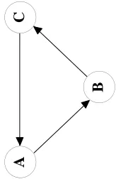
Agraph is formally a pairG= (V, E)where the elements ofV are calledvertices (ornodes) and the elements ofE are callededges orlines. The most informative object of the procedure is the Directed Acyclic Graph (DAG), in which directed edges (arrows) link initial nodes (or

parents) toterminal nodes (orchildren). Figure 1.C2 shows a typical and simple DAG, where nodes A, B and C represent random variables and the directed edges connecting A and B, and B and C indicate the direction of a statistical causality. When undirected edges replace the arrows of a graph, a Conditional Independence Graph (CIG) is obtained. In a CIG, a link represents a significant partial correlation between any two random variables conditional on all the remaining variables of the model. Figure 1.A shows an example of a CIG. The edge connecting nodes A andB represents a significant partial correlation between A and B

conditional on C, while the edge connecting nodes B and C represents a significant partial correlation betweenB and C conditional onA. In Figure 1.A, the absence of an edge linking

Aand C implies that, if A,B and C are distributed as a multivariate Gaussian distribution,

Aand C are independent conditional on B, hence the name CIG.

DAGs and CIGs imply a different definition of joint probability. For example if we consider a DAG such as the one in Figure 1.C2, this has a joint distribution equal to:

while if we take a CIG such as the one in Figure 1.A, we can assert that A and C are independent, conditional on B. Therefore, the implied joint distribution is the following:

fA,C|B(·) =fA|B(·)fC|B(·).

However, there is a correspondence between the two, represented by the so-calledmoralization rule, as firstly shown by Lauritzen and Spiegelhalter (1988), who introduced the verb “marry-ing” instead of “link“marry-ing” two nodes and defined a graph where two parents of a common child are married (i.e. linked) to be moral. The moralization rule states that, in order to derive a unique CIG from a given DAG, arrows should be transformed into undirected edges and unlinked parents of a common child should be linked with an edge. In other words, when two nodes jointly cause a third node and they do not cause each other, from a statistical point of view, there will be a significant correlation between the two. In the DAG shown in Figure 1.B1,A and C are parents of B and do not cause each other. In order to obtain the corresponding unique CIG, arrows must be transformed into edges and a moral edge has to be added between parents A and C as in Figure 1.B2. Putting it differently, when both A

andC determine B, a significant partial correlation (due to moralization) should be observed betweenA and C.2

While there is a unique CIG deriving from a given DAG, the reverse is not true. What the econometrician can observe in the data is a CIG, where every edge can assume two possible directions. Therefore, for any given CIG, there are 2n hypothetical DAGs, where n is the number of edges. Figure 1.C shows all the hypothetical DAGs corresponding to the CIG in Figure 1.A. The DAG in Figure 1.C1 is not compatible with the CIG, because the moralization rule requires a moral edge betweenAand C, which is not captured by the CIG.3

2

While the reader is referred to Lauritzen and Spiegelhalter (1988) for a formal proof of the moralization rule, an example should provide an intuitive insight into the issue: if one wants to become a famous football player (P), he/she must gifted with good skills (S) and/or must work hard (W). ThereforeS andW are the causes ofP. Suppose that we know that one individual did not work hard. Thisper se does not provide any information on whether he/she had good skills. However if the individual is a famous football player, the only thing we can conclude is that he/she had good skills. Therefore, observingP – which is the effect and not the cause ofS andW – is crucial in establishing the partial correlation betweenS andW.

3_{In the process of obtaining plausible DAGs from an observed CIG, it may also be possible that some of}

Any DAG, by definition, has to satisfy the principle of acyclicality. Therefore, the graph depicted in Figure 2 cannot be a DAG as it is clearly cyclic. The acyclicality in a DAG allows to completely determine the distribution of a set of variables and implies a recursive ordering of the variables themselves, where each element in turn depends on none, one or more elements. For example, in the DAG in Figure 1.C2, A depends on no other variables, B depends on A

andC on B.

2.2 Identification of a SVAR with graphical modelling

GM theory can be applied to obtain identification of a structural VAR (SVAR), as shown by Reale and Wilson (2001) and Oxley et al. (2009) among others.

Any SVAR may be turned into a DAG where current and lagged variables are represented by nodes and causal dependence by arrows. After collecting the endogenous variables of interest in the k-dimensional vectorXt, the associated reduced-form, or canonical, VAR can

be written as:

Xt=A(L)Xt−1+ut, (1)

whereA(L)is a polynomial in the lag operatorLandutis ak-dimensional vector of

reduced-form disturbances withE[ut] = 0and E[utu′t] = Σu.

As reduced-form disturbances are correlated, in order to identify structural shocks, the reduced-form model has to be trasformed into a structural model. Pre-multiplying both sides of equation (1) by the(k×k) matrixA0, yields the structural form:

A0Xt=A0A(L)Xt−1+Bet. (2)

The relationship between the structural disturbancesetand the reduced-form disturbancesut

is described by the following:

A0ut=Bet, (3)

Suchdemoralization process, in most cases, can be assessed by considering some quantitative rules. Let us suppose we observe a CIG such as the one in Figure 1.B2. If the true corresponding DAG were the one in Figure 1.B1, then the partial correlation betweenAandC,ρ(A,C|B), should be equal to−ρ(A,B|C)×ρ(B,C|A).

whereA0 also describes the contemporaneous relations among the endogenous variables and

B is a(k×k) matrix. In the structural model, disturbances are assumed to be uncorrelated with each other. In other words, the covariance matrix of the structural disturbances Σe is

diagonal.

As it is, the model described by equation (2) is not identified because there may be possibly many matrices A and B that satisfy (2). Therefore, first matrix B can be restricted to be a (k×k) diagonal matrix. Second, in order to impose identifying restrictions on matrix A0,

graphical modeling theory can be applied to trace DAGs of the contemporaneous variables. The acyclicality of DAGs implies a recursive ordering of the variables that makes A0 a

lower-triangular matrix. A0has generally zero elements also in its lower triangular part, hence,

in general, the model is over-identified. The GM methodology has the distinctive feature that the variable ordering and any further restrictions come from statistical properties of the data. First, as shown by Oxley et al. (2009) in order to construct the CIG among contem-poraneous variables one has to derive the sample partial correlation between each pair of contemporaneous variables, conditioned on the values of the remaining contemporaneous vari-ables and the lagged values of all varivari-ables. This can be computed from the inverseWˆ of the sample covariance matrixVˆ:

ˆ

ρ(xi,t, xj,t|{xk,t}) =−

ˆ Wij

√

( ˆWiiWˆjj)

, (4)

where{xk,t} is the whole set of variables excluding the two considered. Whenever a sample

correlations are obtained, they suggest utilising prior economic information in order to draw a causal order. As also remarked by Swanson and Granger themselves, the structural form of dependence between variables is equivalent to a DAG. With GM and its rules, starting from pairwise partial correlations, it is possible to construct a CIG which imply data-determined constraints on permissible DAGs. As a result, the approach offers a data-driven systematic procedure that leads to the selection of the best DAG, which has the interpretation of statistical causation (or linear predictability in the context of a SVAR).

All possible DAGs (satisfying the moralization rule) which represent alternative compet-itive models are compared via likelihood based methods – such as the Akaike Information Criterion (AIC), the Hannan and Quinn Information Criterion (HIC) or the Schwarz Informa-tion Criterion (SIC) – and/or based on their out-of-sample forecasting performances, and the best-performing one is chosen. In order to construct an empirically well-founded SVAR, one has to assure that the covariance matrix of the resulting residuals is diagonal. A first diagnostic check is thus inspecting the significance of such correlations. Further diagnostic checks are advisable. For instance, as this procedure typically entails the imposition of over-identifying restrictions, aχ2 likelihood-ratio test should be conducted.4

3

Data

The empirical analysis presented in the remainder of the paper employs quarterly US data over the period 1965:1-2007:4. The starting year coincides with that used by Christiano et al. (1999, 2005) while the end date falls in a pre-crisis quarter.

The model is a four-variable VAR including: (i) the log of real GDP, yt; (ii) the effective

federal funds rate (quaterly average),rt; (iii) the log the GDP implicit price deflator, pt, and

(iv) the log of the quarterly average of a commodity price index (producer price index),cpt.

The variables are representative of the real activity, monetary policy and price dynamics.

4_{In some cases, the distributional properties of the variables for different DAGs are likelihood equivalent,}

Such a model specification represents a minimal setting similar to those adopted by Stock and Watson (2001) – for illustrative purposes – and by more recent contributions such as Primiceri (2005) and Koop et al. (2009). The addition of a commodity price proves helpful in ruling out theprice puzzle.5 Giordani (2004) argues that the commodity price index solves the price puzzle not because it is useful in forecasting inflation (as it is often argued in the literature), but rather because it is correlated with the output gap (typically omitted in VARs). In the context of this paper, the commodity price index represents a high-frequency variable the central bank looks at and, in accordance with Giordani (2004), this variable may act as an indicator of the state of the business cycle. The absence of monetary aggregates is due to a preference for parsimony coupled with the fading role of monetary aggregates in the conduct of monetary policy as empirically shown by Estrella and Mishkin (1997), among others, and theoretically explored by Woodford (2008).

A constant is included in the VAR and results are reported both for a VAR in levels, with and without a deterministic trend,6 and for a VAR in which the logs of GDP, the GDP deflator and the commodity price index have been first differenced. The sampling properties of GM are valid regardless of the presence of unit roots in the data, as shown by Wilson and Reale (2008). In fact, we show below that the three model specifications give rise to the same CIGs and DAGs.

All series are extracted from the ALFRED database of the Federal Reserve Bank of St. Louis. The commodity price index was adjusted for seasonality using the Census X12 method, while the other variables were seasonally adjusted by the source.

5

The termprice puzzleis due to Sims (1992). Christiano et al. (1999) show that omitting a commodity price index from the VAR specification delivers a rise in the price level that lasts several years after a contractionary monetary policy shock.

6_{We prefer to report results for both cases, as in the literature both options are explored. For instance,}

rt yt pt cpt rt yt pt cpt

rt 1.000 rt 1.000

yt 0.183* 1.000 yt 0.185** 1.000

pt 0.121 -0.096 1.000 pt 0.062 -0.121 1.000

cpt 0.202*** -0.067 0.387*** 1.000 cpt 0.211*** -0.016 0.435*** 1.000

(a) Model in first differences (b) Model in levels

rt yt pt cpt

rt 1.000

yt 0.219** 1.000

pt 0.011 -0.088 1.000

cpt 0.220*** -0.026 0.439*** 1.000

(c) Model in levels with deterministic trend

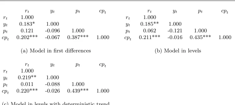
Note: *,** and *** denote significance at 0.10, 0.05 and 0.01 levels, respectively. The corresponding threshold values for the baseline model are 0.1270, 0.1504 and 0.1963, respectively.

Table 1: Estimated partial correlations of the variables

4

Results

DAGs are obtained by fitting the data to equation (1). The lag order is selected via the AIC.7 Table 1 reports the estimated partial correlation matrices of the series and their significance at 0.10, 0.05 and 0.01 levels. The partial correlation matrices are constructed by computing the sample correlations between each pair of contemporaneous variables, conditioned on the values of the remaining contemporaneous variables and the lagged values of all variables.

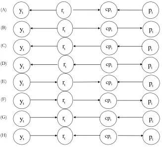
Both the matrix coming from the model in first differences and those coming from the model in levels (with and without trend) translate into the same CIG depicted in Figure 3. The three edges in the CIG cannot be moral, as moral edges link parents of a common child. The 23 _{= 8 possible DAGs implied by the CIG are reported in Figure 4. The moralization}

rule implies that DAGs (A), (E), (G) and (H) can be discarded as they are not compatible with the observed CIG. In fact, in (A) and (E), rt and pt are parents of common child cpt,

which would imply a moral edge betweenrtandptthat does not appear in the observed CIG.

7

In (G) and (H), yt and cpt are parents of common childrt, which would imply a moral edge

betweenyt and cpt that again does not appear in the observed CIG.

(A) (B) (C) (D) (E) (F) (G) (H) t

p

r

y

p

r

y

p

r

y

p

r

y

p

r

y

p

r

y

p

r

y

p

r

y

Figure 4: All possible DAGs deriving from the estimated CIG

The four remaining models are compared via the information criteria mentioned in Section 2. Table 2 shows that the three information criteria for all model specifications are minimised by the model implied by DAG (C), which in turn implies that, within the same quarter, the Federal funds rate is not affected by shocks to the general price level and the real output, while it is affected by shocks to the commodity price.

1980:1-2007:4, i.e. conditional only on the information up to the date of the forecast and with subsequent reestimation every time a new observation was included in the sample.

Model AIC HIC SIC Model AIC HIC SIC

B -418.56 -398.24 -368.48 B -466.06 -445.74 -415.98 C -453.05 -433.17 -403.42 C -521.79 -501.46 -471.71 D -358.26 -337.94 -308.19 D -484.43 -464.11 -434.35 F -405.32 -385.00 -355.24 F -471.50 -451.17 -421.42

(a) Model in first differences (b) Model in levels

Model AIC HIC SIC

B -469.87 -444.47 -407.27 C -525.34 -499.94 -462.74 D -488.20 -462.79 -425.60 F -463.66 -438.26 -401.06

(c) Model in levels with deterministic trend

Note: AIC = Akaike Information Criterion; HIC = Hannan-Quinn Information Criterion (HIC); SIC = Schwarz Information Criterion.

Table 2: Information criteria associated to feasible DAGs

FD LEV LEV-TR FD LEV LEV-TR

B/C 1.24 1.14 1.13 B - C 2.84** 1.70* 1.30 D/C 1.18 1.02 1.02 D - C 2.22** 3.44** 4.13** F/C 1.26 1.04 1.06 F - C 3.05** 1.03 1.15

(a) Ratios of A-MSFEs (b) Diebold-Mariano test statistics

Note: FD = Models in first differences; LEV = Models in levels; LEV-TR = Models in levels with deterministic trend;

A-MSFE = Average Mean Square Forecast Error

* and ** indicate significance of the Diebold-Mariano test statistics at 0.05 and 0.10, respectively.

Table 3: Out-of-sample predictability associated to feasible DAGs relative to model (C) over 1980:1-2007:4.

ϵrt ϵ y

t ϵ

p

t ϵ

cp

t ϵ

r

t ϵ

y

t ϵ

p

t ϵ

cp t

ϵr

t 1.000 ϵrt 1.000

ϵyt 0.026 1.000 ϵ

y

t 0.022 1.000 ϵpt 0.092 -0.112 1.000 ϵ

p

t 0.036 -0.144 1.000 ϵcpt -0.043 -0.048 0.000 1.000 ϵ

cp

t -0.018 -0.020 0.000 1.000

(a) Model in first differences (b) Model in levels

ϵr

t ϵ

y

t ϵ

p

t ϵ

cp t ϵrt 1.000

ϵyt 0.020 1.000

ϵpt 0.035 -0.146 1.000

ϵcpt -0.018 -0.010 0.000 1.000

(c) Model in levels with deterministic trend

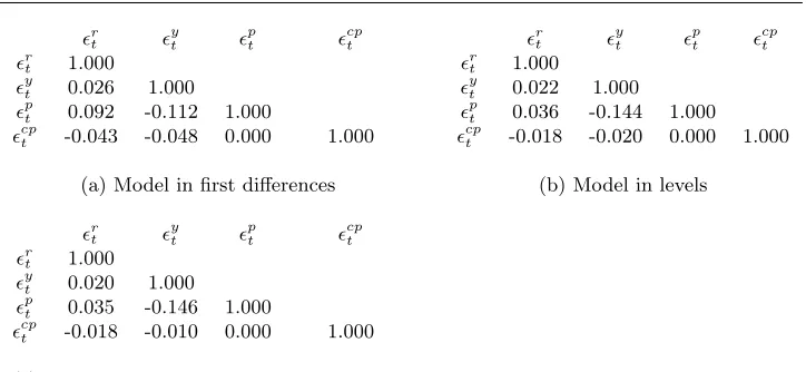
Note: The two-standard-error band for a sample size of 204 is±0.1538

Table 4: Correlations between residuals of the DAGs fitted to the VAR estimated innovations

forecast accuracy of model C is highest in every specification given that the ratios are all larger than unity. To take the possible uncertainty around parameter estimates into account, the models are compared also by means of the Diebold-Mariano (DM) test (Diebold and Mariano, 1995). Table 3b reports the DM test statistics computed on the differences between the MSFE of each competing model and that of model (C). In accordance with Table 3a, the test statistics are systematically positive. The null hypothesis of zero difference is rejected in most cases, at least at a 0.10 significance level. In particular, for the models in first differences the null is always rejected at a 0.05 level. As shown by Inoue and Kilian (2006), a biunivocal correspondence between model rankings based on (in-sample) information criteria and (out-of-sample) forecast errors, does not always hold. In the specific case of this paper, however, it is reassuring to observe that model comparisons made with out-of-sample methods clearly go into the direction of corroborating the results obtained via in-sample criteria.

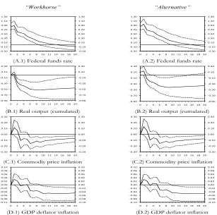
overidentying restrictions which are not rejected at any conventional significance level. For the sake of completeness, Figure 5 reports the impulse responses to a positive Federal funds rate shock obtained by adopting both the “workhorse” and the “alternative” identifica-tion approaches, the latter being consistent with GM. The two approaches generate impulse responses with small quantitative differences, although real output shows a faster and longer lived response with the workhorse approach compared to the alternative approach.

5

Conclusion

The empirical approaches aiming at identifying monetary policy shocks can be classified into two groups: the “workhorse” approach, which assumes that the central bank has sufficient information to accurately infer what contemporaneous real output and GDP deflators are when it takes the monetary policy decision; and the “alternative” approach, which assumes that only variables observed with high frequency, such as commodity prices, are in the information set of the central bank at the time of policy setting. This paper makes use of GM theory to identify a small-scale VAR of the US economy and finds that the application of such a data-based tool give rise to identifying restrictions consistent with the “alternative” approach. When impulse-response analysis is concerned, however, the “workhorse” approach and the model identified by imposing restrictions suggested by GM – coinciding with the “alternative” approach – generate responses to a Federal funds rate shock featuring only small quantitative differences, although real output shows a faster and longer lived response with the workhorse approach compared to the alternative approach.

References

Bernanke, B. S. (1986). Alternative explanations of the money-income correlation. Carnegie-Rochester Conference Series on Public Policy, 25(1):49–99.

Christiano, L. J., Eichenbaum, M., and Evans, C. (1996). The effects of monetary policy shocks: Evidence from the flow of funds. The Review of Economics and Statistics, 78(1):16– 34.

Christiano, L. J., Eichenbaum, M., and Evans, C. (1999). Monetary policy shocks: What have we learned and to what end? In Woodford, M. and Taylor, J. B., editors, Handbook of Macroeconomics, volume 1, chapter 2, pages 65–148. Elsevier, North Holland: Amsterdam.

Christiano, L. J., Eichenbaum, M., and Evans, C. (2005). Nominal rigidities and the dynamic effects of a shock to monetary policy. Journal of Political Economy, 113(1):1–45.

Clarida, R. H., Sarno, L., Taylor, M. P., and Valente, G. (2006). The role of asymmetries and regime shifts in the term structure of interest rates. The Journal of Business, 79(3):1193– 1224.

Darroch, J. N., Lauritzen, S. L., and Speed, T. P. (1980). Markov fields and log-linear inter-action models for contingency tables. The Annals of Statistics, 8(3):522–539.

Dempster, A. P. (1972). Covariance selection. Biometrics, 28(1):pp. 157–175.

Diebold, F. X. and Mariano, R. S. (1995). Comparing predictive accuracy.Journal of Business & Economic Statistics, 13(3):253–63.

Estrella, A. and Mishkin, F. S. (1997). Is there a role for monetary aggregates in the conduct of monetary policy? Journal of Monetary Economics, 40(2):279–304.

Fragetta, M. and Melina, G. (2011). The effects of fiscal policy shocks in SVAR models: A graphical modelling approach. Scottish Journal of Political Economy, 58(4):539–567.

Garratt, A., Lee, K., Pesaran, M. H., and Shin, Y. (2003). A long run structural macroecono-metric model of the UK. Economic Journal, 113(487):412–455.

Hall, P. (1992). The Bootstrap and Edgeworth Expansion. Springer-Verlag, New York.

Inoue, A. and Kilian, L. (2006). On the selection of forecasting models. Journal of Economet-rics, 130(2):273–306.

Kilian, L. (2001). Impulse response analysis in vector autoregressions with unknown lag order.

Journal of Forecasting, 20(3):161–79.

Kim, S. and Roubini, N. (2000). Exchange rate anomalies in the industrial countries: A solution with a structural VAR approach. Journal of Monetary Economics, 45(3):561–586.

Koop, G., Leon-Gonzalez, R., and Strachan, R. W. (2009). On the evolution of the monetary policy transmission mechanism. Journal of Economic Dynamics and Control, 33(4):997 – 1017.

Lauritzen, S. L. and Spiegelhalter, D. J. (1988). Local computations with probabilities on graphical structures and their application to expert systems. Journal of the Royal Statistical Society. Series B (Methodological), 50(2).

Oxley, L., Reale, M., and Wilson, G. (2009). Constructing structural VAR models with conditional independence graphs. Mathematics and Computers in Simulation, 79(9):2910– 2916.

Primiceri, G. E. (2005). Time varying structural vector autoregressions and monetary policy.

Review of Economic Studies, 72(3):821–852.

Reale, M. and Wilson, G. (2001). Identification of vector AR models with recursive structural errors using conditional independence graphs. Statistical Methods and Applications, 10:49– 65.

Sims, C. A. (1992). Interpreting the macroeconomic time series facts : The effects of monetary policy. European Economic Review, 36(5):975–1000.

Stock, J. H. and Watson, M. W. (2001). Vector autoregressions. Journal of Economic Per-spectives, 15(4):101–115.

Swanson, N. R. and Granger, C. W. J. (1997). Impulse response functions based on a causal approach to residual orthogonalization in vector autoregressions. Journal of the American Statistical Association, 92(437):pp. 357–367.

Wilson, G. T. and Reale, M. (2008). The sampling properties of conditional independence graphs for I(1) structural VAR models. Journal of Time Series Analysis, 29(5):802–810.

(A) A C

IG

(B1)

(B2)

(B) A DAG and its corresponding CIG

(C1)

(C2)

(C3)

(C4)

(C) Hypothetical DAGs deriving from CIG in (A)

A

B

C

A

B

C

A

B

C

A

B

C

A

B

C

A

B

C

A

B

C

Figure 1: Conditional independence graphs and directed acyclic graphs

A

B

C

t

p

r

y

Figure 3: Sample CIG

“Workhorse” “Alternative”

(A.1) Federal funds rate (A.2) Federal funds rate

(B.1) Real output (cumulated) (B.2) Real output (cumulated)

(C.1) Commodiy price inflation (C.2) Commodity price inflation

(D.1) GDP deflator inflation (D.2) GDP deflator inflation

! !"#$" !"#%" "#%" "#$" "#&" "#'" "#(" %#%" %#$" !"#$" !"#%" "#%" "#$" "#&" "#'" "#(" %#%" %#$"

" ) * + , %"%) %*%+ %, )"

!"#$" !"#%" "#%" "#$" "#&" "#'" "#(" %#%" %#$" !"#$" !"#%" "#%" "#$" "#&" "#'" "#(" %#%" %#$"

" ) * + , %" %) %*%+ %, )"

!"#$" !"#%" !"#&" !"#'" !"#(" "#(" "#'" !"#$" !"#%" !"#&" !"#'" !"#(" "#(" "#'"

" ) * + , ("() (*(+ (, )" !"#$" !"#%" !"#&" !"#'" !"#(" "#(" "#'" !"#$" !"#%" !"#&" !"#'" !"#(" "#(" "#'"

" ) * + , (" () (*(+ (, )"

!"#$" !"#%" !"#&" "#"" "#&" "#%" "#$" !"#$" !"#%" !"#&" "#"" "#&" "#%" "#$"

" % ' ( ) &"&% &'&( &) %"

!"#$" !"#%" !"#&" "#"" "#&" "#%" "#$" !"#$" !"#%" !"#&" "#"" "#&" "#%" "#$"

" % ' ( ) &" &% &'&( &) %"

!"#$" !"#"% !"#"& !"#"' !"#"( "#"" "#"( "#"' "#"& "#"% "#$" !"#$" !"#"% !"#"& !"#"' !"#"( "#"" "#"( "#"' "#"& "#"% "#$"

" ( ' & % $"$( $'$& $% ("

!"#$" !"#"% !"#"& !"#"' !"#"( "#"" "#"( "#"' "#"& "#"% "#$" !"#$" !"#"% !"#"& !"#"' !"#"( "#"" "#"( "#"' "#"& "#"% "#$"

" ( ' & % $" $( $'$& $% ("

Note: Dashed lines represent 90% confidence intervals computed according to Hall (1992) algorithm with 2000 bootstrap replications. Responses are shown for a 20-quarter horizon.