Identification of broadband source-array responses from sensor second order statistics

Identification of Broadband Source-Array

Responses from Sensor Second Order Statistics

S. Weiss

, N.J. Goddard

, S. Somasundaram

, I.K. Proudler

, and P.A. Naylor

†_{DSTL Portsdown, Fareham, Hampshire PO17 6AD, UK} ‡_{Thales Underwater Systems, Cheadle, Stockport SK3 0XB, UK}

§_{School for Mechanical, Electrical and Manufacturing Eng., Loughborough University, Leicestershire LE11 3TU, England} ¶_{Dept. of Electrical & Electronic Engineering, Imperial College London, London SW7 2AZ, UK}

e-mail: [email protected]

Abstract—This paper addresses the identification of

source-sensor impulse responses from the measured space-time covari-ance matrix in the absence of any further side information about the source or the propagation environment. Using polynomial matrix decomposition techniques, the responses can be narrowed down to an indeterminacy of a common polynomial factor. If at least two different measurements for a source with constant power spectral density are available, this indeterminacy can be reduced to an ambiguity in the phase response of the source-sensor paths.

I. INTRODUCTION

Second order statistics of sensor array data have been used in numerous ways to characterise signal processing parameters. In the case of sources in the array’s far-field, and in the absence of multipath propagation, for example the angles of arrival can be estimated for both narrowband [1], [2] and broadband signals [3]–[5]. For near-field or multipath propagation, signal parameters have been extracted for the narrowband case, see e.g. [6], but the broadband approach is more difficult and often can only be made sufficiently robust to multipath effects without directly exploiting or extracting these [7].

However, the extraction of parameters such as a source’s power spectral density (PSD), as well as multipath charac-teristics of the transfer paths can be usefully exploited to obtain clues about the propagation environment, which in turn can assist in locating a source. For example, in [8] a model of the propagation environment has been extracted from a single impulse response. Similarly, impulse responses of a single input multiple output sysyte can be utilised to infer the geometry of an acoustic room [9] or attempt to acoustically image the propagation environment and locate the source [10]. Therefore, this paper investigates to which extend poly-nomial matrix decomposition techniques [11] can assist in resolving the desired impulse responses. To do this, Sec. II describes the model for the scenario, and the data that is acquired. Sec. III reviews the polynomial eigenvalue decompo-sition (PEVD) and ambiguities associated with its polynomial matrix factors. Sec. IV outlines that with the source in a single position, not much can be determined. If measurements include a relocation of the source (by either movement of the

source or the sensor array), then the source power spectral density and the magnitude responses of the transfer paths can be extracted, as demonstrated in Sec. V. While this leaves us with a phase ambiguity, the polynomial approach is still capable to retrieve significantly more information than a frequency-bin approach would be capable of achieving, as shown in Sec. VI. A numerical example is provided in Sec. VII.

II. SOURCEMODEL

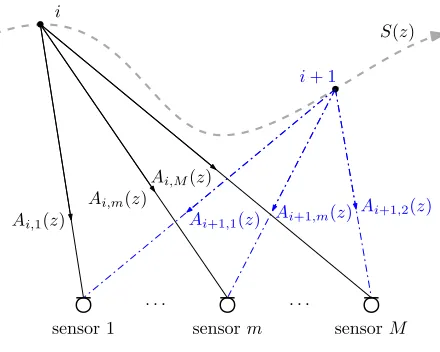
We assume a single source that illuminates anM-element sensor array as shown in Fig. 1. The transfer functions between the source and the sensor elements are contained in a vector

ai(z)∈CM,

a_i(z) =



 

Ai,1(z)

.. .

Ai,M(z)





 , (1)

where i is a measurement campaign index. A measurement campaign is here defined as a data acquisition over a brief period of time over which the propagation paths between source and array are stationary, such that transfer functions as shown in (1) can be defined. The source is assumed to be wide sense stationary with a PSD S(z). From one measurement campaign to the next, a variation of the transfer functions in a_i(z) is expected to occur and may arise from a relative change between the source and the sensor array, i.e. either through a movement of the source, a change in the array’s position, orientation, or configuration, or through a change in the propagation environment.

If the sensor signals are collected in a vector x_i[n] ∈

CM_{, then the sensor covariance matrix is R}

i[τ] =

E

xi[n]xHi [n−τ] . The cross-spectral density (CSD) during

thisith campaign is

R_i(z) =

∞

X

τ=−∞

R_i[τ]z−τ (2)

=ai(z)S(z)aPi(z) +σ

2

nIM (3)

whereσ2

nis the power of spatially and temporally uncorrelated

A_i;1(z)

A_i;m(z₎

A_i+1;2(z)

A_i+1;1(z)

S₍z₎ i

i+ 1

A_i;M(z₎

A_i+1;m(z)

sensor 1 sensorm sensorM

: : : : : :

Fig. 1. Model with source power spectral densityS(z)and two measurements campaigns along the source’s trajectory relative to the sensor array with transfer functions Ai,m(z),m= 1. . . M, between the source and theM

sensors.

operator, such that aP

i(z) = aH(1/z

∗

) is the Hermitian transposed time-reversed version of a(z). Because of its dependence on z, the CSD matrix R(z) is referred to as a polynomial matrix. WithR[τ]in (3) being composed of auto-and cross-correlation terms, due to its inherent symmetryR(z) represents a parahermitian matrix, such that R(z) =RP(z). This property is an extension of the symmetric or Hermitian property of real and complex-valued matrices, respectively, to the ring of polynomial matrices.

We assume that the source maintains the same power spectral density, but that due to non-stationarity or movement of the source, the vector of transfer functions changes between measurement campaigns.

III. POLYNOMIALEIGENVALUEDECOMPOSITION

The eigenvalue decomposition (EVD) of Hermitian matrices is a central operation in signal processing, and below we will discuss some aspects of defining an extension of the EVD to parahermitian polynomial matrices, called a polynomial EVD (PEVD) [11].

A. Existence

For a parahermitian matrix R(z), the PEVD currently has not yet been proven to exist, but it is claimed that a good approximation by means of FIR paraunitary matrix factorQ(z)and a diagonal and spectrally majorisedΛ(z)of sufficient order can be found [12], such that the PEVD [11] or McWhirter decomposition

R(z)≈Q(z)Λ(z)QP(z) (4)

holds. Spectral majorisation implies that when evaluat-ing the polynomial eigenvectors contained in Λ(z) = diag{λ0(z) . . . λM−1(z)} on the unit circle, the power

spec-tral densities fulfil

λm(ejΩ)≥λm+1(ejΩ) ,∀Ω m= 0. . .(M −2). (5)

This restricts an ambiguity of the decomposition w.r.t. a potential frequency-dependent permutation of eigenvalues and -vectors.

Instead of spectral majorisation, if an analytic R(z) is evaluated on the unit circle, R(ejΩ_{) = R(z)|}

z=ejΩ, Fourier

domain factors for eigenvalues and -vectors can be selected analytic inΩ[13]. These can be extended to eigenvalues and -vectors that are analytic, i.e. maximally smooth, functions in

z. This now enables an exact decomposition with equality (4), but must be based on Laurent series, since the factorsΛ(z)and

Q(z) may be of infinite length i.e. potentially transcendental functions inz. Below, we assume that such an analytic rather than a spectrally majorised PEVD is selected, and exists with equality in (4).

The columns of Q(z) are the polynomial eigenvectors

um(z),

Q(z) =

q0(z) . . . q_M−1(z)

. (6)

Based on the polynomial eigenvalues and -vectors, the PEVD can also be written as

R(z)≈

M−₁

X

m=0

λm(z)qm(z)q

P

m(z). (7)

B. Ambiguity

To explore ambiguity, we assume that the PEVD in (7) exists with equality. For the eigenvectors,

q_m(z)qP_n(z) =δ(n−m), (8)

holds withm, n= 1. . . M. They can be modified as

q′_m(z) =Um(z)qm(z), (9)

by an arbitrary allpass filterU(z), such that theq′

m(z),m=

0. . .(M−1) will still form valid eigenvectors satisfying (8). This allpass filter must be common to all elements ofq_m(z), and can in the simplest case form a delay [14]. Note that thereforeq_m(z)andq′_m(z)will have an identical magnitude but different phase responses.

This ambiguity is a generalisation of the ambiguity of eigenvectors of a non-polynomial eigenvalue problem, where both sides of Av = λv can be multiplied by an arbitrary phase shiftejϕ_{, such thatv}′

=vejϕ _{akin to (9).}

C. Iterative PEVD Algorithms

Iterative PEVD algorithms currently belong to the families of sequential best rotation (SBR2) [11] and sequential ma-trix diagonalisation (SMD) [15] algorithms. These perform an approximate iterative diagonalisation by FIR paraunitary factors. The type of rational function represented by an allpass filter implementing an arbitrary phase response is likely to be approximated by a large number of zeros. This ambiguity in (8) may be hidden, but motivates the comparison of transfer functions across every eigenvector q_m(z), m = 1. . . M of

Q(z)for common zeros, and particular delays [14].

case of SBR2 can even be proven [16]. In case that eigenvalues intersect on the unit circle, spectral majorisation will enforce the approximation of non-analytic eigenvalues and -vectors. To guarantee analytic eigenvalues even in case of eigenvalues intersecting on the unit circle, algorithms different from SBR2 or SMD are required, with a DFT-base approach in [17] a first step.

IV. EXTRACTIONBASED ON ASINGLECAMPAIGN

We assume that for a single measurement campaigni, the CSD matrix R_i(z)according to (2) has been estimated, and its PEVD exists and is known, such that

R_i(z) =

q_i(z)q⊥_i (z)

γi(z) +σn2

σ2

nIM−₁

qP_i(z)

q⊥_i,P(z)

(10) =q_i(z)γi(z)qPi(z) +σ

2

nIM . (11)

The difference between the source model in (3) and the PEVD in (11) is that q_i(z) is by definition normalised whileai(z)

is unnormalised,

qP_i(z)q_i(z) = 1 (12)

aP_i(z)a_i(z) =Ai(z) =A

(+)

i (z)A

(−)

i (z) (13)

=A(+)_i (z)A_i(+),P(z), (14) whereAi(z)is a PSD andAi[τ]◦—•Ai(z)has the symmetry

properties of an auto-correlation function, i.e.Ai(z) =APi(z),

andA(+)_i (z)is the minimum-phase part ofAi(z). It is assumed

thatAi(z)has no spectral zeros. Normalisation of ai(z)can

therefore be accomplished by setting

a_i,norm(z) = ai(z)

A(+)_i (z). (15)

With this normalisation, (3) can be rewritten as

R_i(z) =a_i,norm(z)A(+)_i (z)S(z)A(+)_i ,P(z)aP_i,norm(z) +σ2

nIM.

(16) Comparing (16) to (11), with γi(z)the dominant eigenvector

minus the noise floor in the PEVD in (11), we can extract

q_i(z) = ai(z)

A(+)_i (z) (17)

γi(z) =A

(+)

i (z)S(z)A

(+),P

i (z), (18)

such that the vector of transfer functions and the source power spectral density can be determined except for unknown scaling factors1/A(+)_i (z)andA_i(+)(z)A(+)_i ,P(z), respectively, and the phase-indeterminacy inherent in the eigenvectors of the PEVD.

V. EXTRACTIONBASED ONMULTIPLECAMPAIGNS

Instead of a single campaign, now multiple measurement campaigns have been performed and the decompositions (17) and (18) are available fori= 1. . . I. If there are no roots that are common to allA(+)_i (z), then the source PSD represents the greatest common divisor (GCD) across all instances of (18),

ˆ

S(z) =GCD{γ1(z) . . . γI(z)}. (19)

From this, estimates of the scaling termsAˆ(+)_i (z) remaining in (17) and (18) can be extracted for every measurement campaign.

The estimation of the scaling termAˆ(+)_i (z)now leads to a more precise estimate of the source-array transfer functions from (17), whereby only an indeterminacy remains in the phase response for every aˆ(z) due to the ambiguity charac-terised in Sec. III-B, leading to

ˆ

ai(z) = ˆA

(+)

i (z)Ui(z)qi(z) (20)

with Ui(z) an arbitrary allpass filter according to (9). With

the ambiguity restricted to the phase responses, however the magnitude responses of the source-array transfer paths are now fully determined.

The viability of this approach depends on an accurate determination of a GCD, i.e. of finding common zeros across multiple polynomials. This problem has been addressed by Euclid in his 7th book ofElementsaround 300BC [18], by a method referred to as Euclid’s algorithm. Because its robust-ness deteriorates quickly with the order of the polynomials, refinements are still being made to date, see e.g. [19]–[25].

As we will explore through an example in Sec. VII, extract-ing a GCD even for a controlled scenario is difficult based on recent algorithms such a [25]. However, the aim here is to highlight the general approach independent of the problem of root finding, where perhaps robust approaches such as Gr¨obner bases may provide viable future alternatives.

VI. SOLUTION ININDEPENDENTFREQUENCYBINS

Classically, broadband problems are often addressed by solving a number of narrowband or discrete Fourier transform (DFT)-domain problems independently in adjacent frequency bins. In this section, we consider an approach where the input signal is split into K such frequency bins, and compare this as a benchmark to the findings of Secs.IV and V.

ApplyingK-point discrete Fourier transforms to the mea-sured signals, then with sufficient averaging K narrowband covariance matrices Ri,k arise at the normalised angular

frequencies Ωk = 2_Kπk, k = 0. . .(K −1) during the ith

measurement campaign,

R_i,k =R_i(ejΩk_{) =a}

i(ejΩk)S(ejΩk)aHi (ejΩk) +σn2I (21)

=q_i,kλi,kqHi,k, (22)

where Ri(ejΩk) = R(z)|z=ejΩk is the evaluation of (2) on the unit circle for frequencyΩk.

The principal eigenvectors and eigenvalues for the measure-ment campaigns are

q_i,k = ai(e

jΩk)

|a_i(ejΩk)| , (23)

λi,k =S(ejΩk)|ai(ejΩk)|2, (24)

which again are discrete evaluations of (17) and (18) on the unit circle.

0 0.05 0.1 0.15 0.2 0.25 0.3 0.35 0.4 0.45 0.5 −10

−8 −6 −4 −2 0

normalised angular frequency Ω/(2π)

normalised power spectral density / [dB]

S(z) λ

1(z) λ

2(z) λ

1(z)/|A1 (+)_(z)|2

λ 2(z)/|A1

(+)_(z)|2

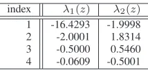
Fig. 2. Source PSDS(z)compared to eigenvalues λi(z)calculated from

R_{i(z)of both measurement campaigns, with the scaled versions to correct}

for (18). All PSDs are normalised to a maximum value of unity.

bins in the independent frequency bin representation has been lost compared to (17) and (18). Also, (23) has an indetermi-nacy w.r.t. angle since adding multiples of2πto the phase and therefore imposing a delay will not change the vector. Part of this indeterminacy could be removed by considering coherence across frequency bins and thus unwrapping the phase; this process is however not directly obvious from (23) and (24), and requires additional processing.

Therefore, without additional processing to account for co-herence between bins, the independent frequency bin method exhibits an indeterminacy in terms of both amplitude and delay, and can retrieve neither the transfer functionsAi,m(z)

nor the source power spectral density S(z).

VII. NUMERICALEXAMPLE

As an example, a source with power spectral density

S(z) = 1 2z+

5 4+

1 2z

−₁

(25)

illuminates an M = 2 element array during measurement campaign i= 1 via the transfer function vector

a1(z) =

1 + 1 2z

−1 3

4 − 1 2z

−1

, (26)

and during measurement campaign i= 2via

a2(z) =

4

5 − 1 2z

−1

−1

2 + z

−1

. (27)

The PSD and various magnitude responses are shown in Figs. 2–4; for easier comparison with some of the calcula-tions further below, the curves are normalised such that their maximum value is unity.

Using the SMD algorithm [15] to estimate the PEVD, the eigenvalues λi(z), i = 1,2 are determined; their PSDs

are displayed in Fig. 2. These bear no resemblance with the source PSD; neither can the principal eigenvectors q_i(z) reveal anything about the source-array transfer functions when considered in isolation. Evaluated on the unit circle, the

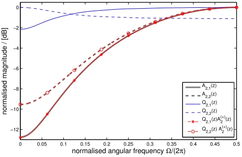
TABLE I

ROOTS OF POLYNOMIAL EIGENVALUESλi(z),i= 1,2.

index λ1(z) λ2(z) 1 -16.4293 -1.9998 2 -2.0001 1.8314 3 -0.5000 0.5460 4 -0.0609 -0.5001

magnitudes responses of the given source-array paths and the determined principal eigenvectors in Figs. 3 and 4 do not match, as expected from Sec. IV.

To identify the common scaling factors across both cam-paigns, we closer inspect the eigenvalues λi(z), i = 1,2.

Since the toy problem is noise-free, we have γi(z) = λi(z)

w.r.t. (11). After trimming the order of the polynomial matrix factors in the PEVD, the principal eigenvalues campaigns both have four roots each as listed in Tab. I. Two roots atz=−2 and z = −1

2 match closely, but do not entirely coincide due to estimation errors by the SMD algorithm as well as due to trimming of the polynomial matrix factors [14]. As a results, root finding algorithms such the one in [25] cannot determine the GCD exactly, and roots here have been matched by inspection.

The matching zeros of Tab. I form the GCD, which now represents the estimate for the source PSD according to (19). This is demonstrated by the close agreement between the orginal and the estimated source PSDs in Fig. 2. From the remaining zeros in Tab. I with |z| < 1, the minimum phase correction factors

A(+)1 (z) = 1 + 0.0609z

−₁

(28)

A(+)2 (z) = 1−0.5460z

−1

(29)

are extracted. These enable the estimation of the transfer function vectors via (20), with ambiguity of the phase response but matching magnitude responses as seen for the paths of campaigni= 1in Fig. 3 and for campaigni= 2in Fig. 4.

VIII. CONCLUSIONS

This paper has explored the possibility of extracting source-sensor paths and source power spectral densities based on the second order statistics of data collected by the sensors only. If only a single measurement is available, the transfer paths have an ambiguity with respect to an unknown common poly-nomial factor, i.e. neither amplitude nor phase response can be determined precisely. By having at least a second measurement campaign — defined as a separate measurement of the same source but with different transfer functions — this ambiguity can in principle be narrowed down to the phase response. We have assumed that multiple measurement campaigns are taken over time, but this can be equally performed spatially, e.g. by partitioning the array.

0 0.05 0.1 0.15 0.2 0.25 0.3 0.35 0.4 0.45 0.5 −15

−10 −5 0

normalised angular frequency Ω/(2π)

normnalised magnitude / [dB]

A 1,1(z) A

1,2(z) Q

1,1(z) Q

1,2(z) Q

1,1(z)A1 (+)_(z)

Q 1,2(z)A1

(+)_(z)

Fig. 3. Transfer functions and principal eigenvector components for measure-ment campaigni= 1, with corrected eigenvectors based on both campaigns.

0 0.05 0.1 0.15 0.2 0.25 0.3 0.35 0.4 0.45 0.5

−12 −10 −8 −6 −4 −2 0

normalised angular frequency Ω/(2π)

normalised magnitude / [dB]

A 2,1(z) A

2,2(z) Q

2,1(z) Q

2,2(z) Q

2,1(z)A2 (+)_(z)

Q 2,2(z) A2

(+)_(z)

Fig. 4. Transfer functions and principal eigenvector components for measure-ment campaigni= 2, with corrected eigenvectors based on both campaigns.

approach, which retains an ambiguity with respect to phase and magnitude even for multiple measurement campaigns due to the negligence of coherence across frequency bins.

Extraction of accurate magnitude responses of the source-sensor paths depends on robustly determining the greatest common divisor across several polynomials. Estimation errors in the covariance matrices and approximations inherent in iterative PEVD algorithms make this difficult, and robust root finding methods will be crucial for developing this approach further. This may well pose practical limitations for the proposed approach, but does not limit the theoretical findings of this paper.

ACKNOWLEDGEMENT

This work was supported in parts by the Engineering and Physical Sciences Research Council (EPSRC) Grant number EP/K014307/1 and the MOD University Defence Research Collaboration in Signal Processing.

REFERENCES

[1] A. Paulraj, R. Roy, and Kailath. A subspace rotation approach to signal parameter estimation. Proc. IEEE, 32(7):984–995, July 1986. [2] R. O. Schmidt. Multiple emitter location and signal parameter

estima-tion. IEEE Trans. Ant. Prop., 34(3):276–280, Mar. 1986.

[3] H. Wang and M. Kaveh. Coherent signal-subspace processing for the detection and estimation of angles of arrival of multiple wide-band sources. IEEE Trans. ASSP, 33(4):823–831, Aug. 1985.

[4] H. Wang and M. Kaveh. On the performance of signal-subspace processing–part ii: Coherent wide-band systems. IEEE Trans. ASSP, 35(11):1583–1591, Nov. 1987.

[5] M. Alrmah, S. Weiss, and S. Lambotharan. An extension of the MUSIC algorithm to broadband scenarios using polynomial eigenvalue decom-position. InEUSIPCO, pp. 629–633, Barcelona, Spain, Aug. 2011. [6] V. Reddy, A. Paulraj, and T. Kailath. Performance analysis of the

optimum beamformer in the presence of correlated sources and its behavior under spatial smoothing. IEEE Trans. on Acoustics, Speech, and Signal Processing, 35(7):927–936, Jul 1987.

[7] W. Liu. A novel approach to adaptive beamforming for multi-path broadband signals. InIEEE Workshop on Statistical Signal Processing, pages 197–200, Aug 2009.

[8] I. Dokmani´c, Y. Lu, and M. Vetterli. Can one hear the shape of a room: the 2-d polygonal case. InIEEE Int. Conference on Acoustics, Speech, and Signal Processing, 2011.

[9] F. Antonacci, J. Filos, M. R. P. Thomas, E. A. P. Habets, A. Sarti, P. A. Naylor, and S. Tubaro. Inference of room geometry from acoustic impulse responses. IEEE Trans. Audio, Speech, and Language Proc., 20(10):2683–2695, Dec. 2012.

[10] L. Remaggi, P. J. B. Jackson, and P. Coleman. Source, sensor and reflector position estimation from acoustical room impulse responses. In22nd Int. Congress Sound & Vibration, Florence, Italy, July 2015. [11] J. G. McWhirter, P. D. Baxter, T. Cooper, S. Redif, and J. Foster.

An EVD Algorithm for Para-Hermitian Polynomial Matrices. IEEE Trans. Signal Processing, 55(5):2158–2169, May 2007.

[12] S. Icart and P. Comon. Some properties of Laurent polynomial matrices. InIMA Conf. Maths in Signal Proc., Birmingham, UK, Dec. 2012. [13] F. Rellich. St¨orungstheorie der Spektralzerlegung. iii. Mitteilung.

Ana-lytische, nicht notwendig beschr¨ankte St¨orung.Mathematische Annalen, 116:555–570, 1939.

[14] J. Corr, K. Thompson, S. Weiss, I. Proudler, and J. McWhirter. Row-shift corrected truncation of paraunitary matrices for PEVD algorithms. In 23rd Europ. Signal Proc. Conf., pp. 849–853, Nice, France, Aug. 2015. [15] S. Redif, S. Weiss, and J. McWhirter. Sequential matrix diagonalization algorithms for polynomial EVD of parahermitian matrices. IEEE Trans. Signal Processing, 63(1):81–89, Jan. 2015.

[16] J. G. McWhirter and Z. Wang. Insight into the SBR2 algorithm. InIMA Conf. Maths in Signal Proc., Birmingham, UK, Dec. 2016.

[17] M. Tohidian, H. Amindavar, and A. M. Reza. A dft-based approximate eigenvalue and singular value decomposition of polynomial matrices. EURASIP J Advances in Signal Proc., 2013(1):1–16, 2013.

[18] Euclid. Euclide’s elements; the whole fifteen books compendiously demonstrated. [. . . ]. Isaac Barrow, London, 1751.

[19] S. Barnett. Greatest common divisor of several polynomials. Math. Proc. Cambridge Philosophical Society, 70:263–268, 9 1971. [20] A. Conflitti. On computation of the greatest common divisor of several

polynomials over a finite field. Finite Fields and Their Applications, 9(4):423–431, 2003.

[21] D. Henrion and M. Sebek. Reliable numerical methods for polynomial matrix triangularization. IEEE Trans. Aut. Contr., 44(3):497–508, Mar. 1999.

[22] E. Kaltofen, Z. Yang, and L. Zhi. Approximate greatest common divisors of several polynomials with linearly constrained coefficients and singular polynomials. In Proc. International Symposium on Symbolic and Algebraic Computation, pages 169–176, New York, NY, 2006. [23] P. van Dooren. Rational and polynomial matrix factorizations via

recursive pole-zero cancellation. Linear Algebra and its Applications, 137-138(0):663–697, 1990.

[24] A.-G. Wu, G.-R. Duan, and Y. Xue. Kronecker maps and sylvester-polynomial matrix equations. IEEE Trans. Automatic Control, 52(5):905–910, 2007.