Convergence of calculated transition loci during computational analysis of transonic aerofoils and infinite swept wings

City, University of London Institutional Repository

Citation

:

computational analysis of transonic aerofoils and infinite swept wings. Paper presented at the 29th Congress of the International Council of the Aeronautical Sciences, ICAS 2014, 7-12 Sep 2014, St Petersburg, Russia.

This is the accepted version of the paper.

This version of the publication may differ from the final published

version.

Permanent repository link:

Link to published version

:

Copyright and reuse:

City Research Online aims to make research

outputs of City, University of London available to a wider audience.

Copyright and Moral Rights remain with the author(s) and/or copyright

holders. URLs from City Research Online may be freely distributed and

linked to.

City Research Online: http://openaccess.city.ac.uk/ [email protected]

Abstract

The effect of intermittent re-calculation of transition position is analysed using a low-order VII platform coupled to an Orr-Sommerfeld-type stability analysis method. Transonic aerofoil and infinite-swept wing flows are studied. Where the transition mechanisms are weakly dependent on the gross flow field characteristics, as few as ten transition updates may be required over a 1000-iteration CFD solution, if correctly timed.

1 Introduction

Within the European research community, the combination of transition prediction models with RANS-type computations was first piloted in the 1990s as a spin-off from the development of low-cost transition prediction codes during the EU-funded laminar flow control projects (e.g. ELFIN, ELFIN 2, HYLDA, HYLTEC, ALTTA). These studies focussed mainly on simple aerofoil and infinite-swept wing test cases for which the early transition prediction codes were well suited. Subsequent work to apply transition prediction to more complex CFD analyses has resulted in the analysis of UCAV configurations [1], [2], transport aircraft in cruise and high-lift configurations [3] and separation-bubble dominated flows [4]. Transition prediction methodologies have included empirical criteria, stability analysis with the semi-empirical eN transition criterion, and intermittency transport equations solved alongside models of turbulence [5].

One of the differences between the modelling of turbulence and transition is that turbulence interacts directly with the wider flow field, by means of mass, momentum and energy transfer, while transition can be thought of as a topological feature with indirect (albeit significant) influence delivered through the varying extent of laminar and turbulent flow. Except for more sophisticated studies such as [4] in which stability results were used to propose initial Reynolds-stress distributions for turbulence transport equations, transition modelling is normally used merely to adjust the position of a virtual transition ‘trip’ at which the source terms in turbulence models are switched on. This distinct influence on the flow admits the possibility of re-calculating the transition locus less frequently than, for example, the Reynolds-stress terms in a RANS simulation.

During the early experiments to include transition modelling in RANS, efforts were always made to employ database-type methods as the computational cost of a full stability analysis usually dwarfed that of the host RANS simulation. The simplest, algebraic transition criteria were usually found to be deficient in cases where the onset of transition was controlled by the tailoring of pressure distributions (natural laminar flow) or by the use of active techniques, such as surface suction (laminar flow control) – or indeed combinations of the two (hybrid laminar flow control). The better database methods were essentially curve fits to stability analysis results and could therefore deliver much more realistic transition

CONVERGENCE OF CALCULATED TRANSITION LOCI

DURING COMPUTATIONAL ANALYSIS OF

TRANSONIC AEROFOILS AND INFINITE SWEPT

WINGS

C J Atkin*

*City University London, UK

C J ATKIN

trends than the simple criteria, but at comparable cost. However, with increasing complexity of laminar flow test cases (involving sweep, flow curvature, suction control) the database methods can become unwieldy as the number of dimensions of the stability problem – and therefore the effort to populate database-type models – increases. As a result it is still common to find full stability analysis codes, of the Orr-Sommerfeld or PSE type, coupled to CFD methods for the purposes of transition prediction. In these cases it is worthwhile to explore whether the analysis of transition can be carried out to a much coarser resolution, both spatially and temporally, than employed for the other fluid phenomena, to avoid soaring computational costs. This is the objective of the present study.

2 Numerical approach

The platform used for the work is the Airbus Callisto code, a turbulent boundary layer method based on the von Karman momentum integral equations, incorporating the Lag-Entrainment model of Green et al. [6], and modelling three-dimensional turbulence using the streamline analogy. The rationale behind the Callisto development was to develop a Lag-Entrainment code which could be coupled to many different inviscid solvers, and indeed to develop an object-oriented (OO) coupling framework which could be exploited by other boundary layer methods. The viscous-coupled approach is described in detail by Lock & Williams [7], and has the advantage of requiring considerably less computing resource than RANS, with comparable accuracy for attached flows, while intrinsically delivering a breakdown of drag into friction, form and wave drag components.

Callisto has now been coupled to a wide range of codes: the BAE Systems codes RANSMB (structured multi-block) and Flite3D (unstructured Euler); Fluent, via UDFs; and the DLR Tau code. The method is accessed by the inviscid solvers as a shared library: this software architecture means that the same modelling, implemented via the same lines of code, is accessed by each method. As well as meeting the re-usability objective for OO software, this approach simplifies the transfer of novel viscous

modelling (for example, flow control) from research-type to industrial methods with some confidence.

Therefore, in order to permit rapid conceptual flow control studies on transonic wing geometries, Callisto was also coupled to the full potential aerofoil method of Garabedian & Korn [8], extended to handle infinite-swept wing flows using Lock’s transformation [9]. Callisto Viscous Garabedian & Korn, or CVGK, is therefore a quasi-3D version of the BVGK method developed at the Royal Aircraft Establishment (RAE) [10]. A recent numerical study conducted by Atkin and Gowree [11] demonstrated that CVGK can predict the drag on swept wings in transonic flow with good accuracy.

Transition modelling is implemented in Callisto by means of further coupling to the QinetiQ boundary layer and stability analysis codes, BL2D and CoDS. BL2D is a classical, finite-difference, parabolic solver of the type described by Horton & Stock [12]. These methods were used, along with BVGK, during the HYLTEC project to assess the performance of a hybrid laminar flow control system fitted to a conventional turbulent wing design [13]. The earlier Lag-Entrainment codes developed by the RAE employed a simple Thwaites method for the laminar part of the boundary layer, and so the coupling with BL2D meets another objective of the OO design of Callisto, namely to facilitate coupling of a number of different boundary layer methods. BL2D is a differential method, whereas the Thwaites and Lag-Entrainment methods are of the integral type: hence the OO framework has also enabled methods of different fidelity to be managed under a single software architecture. Similarly, the coupling with CoDS, a classical linear stability analysis method, introduces a completely different type of numerical algorithm.

back to the inviscid solver in an iterative manner. This then introduces a further convergence metric, the position or locus of transition, to be monitored.

With the recent renewed interest in HLFC (although the suction chamber modelling capability in Callisto will not feature in this paper), it is timely to assess the performance of this coupled suite of codes and, in particular, to explore means of limiting the impact of the higher-fidelity analyses (BL2D and CoDS) on the normally very efficient CPU usage of the underlying, lower-fidelity, turbulent integral method. Essentially this means analysing the laminar parts of the flow, and the transition position, less frequently than the basic turbulent flow which dominates the displacement effect of the boundary layer. Accordingly Callisto allows for intermittent analysis of both the laminar boundary layer mean flow, and – separately – the boundary layer stability.

3 Numerical investigations

The CVGK method has been exercised against three transonic aerofoil test cases: the RAE2822 aerofoil, a case familiar to all transonic CFD practitioners; the RAE5225 aerofoil, with a more ‘classical’ rooftop pressure distribution typical of a turbulent wing design; and the RAE5243 aerofoil, more commonly referenced as the DRA 2303 model, which has a strongly favourable rooftop pressure gradient typical of a natural laminar flow design concept.

The aerofoils have been analysed near to their maximum M.L/D condition, after allowing for additional zero-lift drag which would arise from an aircraft fuselage/empennage, rather than at test conditions explored in the literature, so that the operating Mach, CL and Reynolds

number might be representative of a transport aircraft employing these wing sections. In order to capture sweep effects, the aerofoils have also been yawed at both 20° and 30°, with corresponding increases in cruise Mach and Reynolds number, and corresponding decrease in CL, so that the yawed and 2D test cases are

‘equivalent’ by Lock’s definition [9]. The test case matrix is summarised in Table 1 and the

pressure distributions are plotted in Figures 1, 2 and 3 overleaf.

In each case the tried-and-tested G&K mesh of 160 × 30 (chord-wise and normal) was used; Callisto was called every third G&K (inviscid) cycle; the convergence criterion on residuals was 8 × 10-6 and was satisfied within 8000 inviscid cycles for all test cases.

A range of different intermittency strategies, for the computation of the laminar flow and transition locus, were tried. The most significant strategies are listed in Table 2 below.

The key outputs from these analyses were not the final CFD solutions but rather the convergence histories for the lift force, residuals and transition locus.

Section RAE2822 RAE5225 RAE5243

2D conditions

Mach 0.730 Rec 20.7M CL 0.679

Mach 0.735 Rec 21.7M CL 0.676

Mach 0.670 Rec 19.0M CL 0.740

20° sweep conditions

Mach 0.777 Rec 23.4M CL 0.600

Mach 0.782 Rec 24.8M CL 0.596

Mach 0.713 Rec 21.5M CL 0.653

30° sweep conditions

Mach 0.843 Rec 27.6M CL 0.509

Mach 0.849 Rec 28.9M CL 0.505

Mach 0.773 Rec 25.3M CL 0.555

Fixed transition positions

Upper surface: transition @ 30% chord Lower surface: transition @ 5% chord

Table 1: transonic aerofoil test cases and equivalent infinite swept conditions.

ID Strategy of laminar & transition analysis

stdb BL2D analysis every 10 viscous cycles; fixed transition (no CoDS stability analysis)

lam1 BL2D as above; CoDS every 50 viscous cycles (1, 51, 101, etc.); transition locked to nearest mesh point; transition movement relaxation factor 0.5. lam1a As ‘lam1’, but transition free to locate in between

mesh points.

lam4 BL2D every 5 viscous cycles; CoDS every 20 viscous cycles (1, 21, 41, etc.); transition free to locate in between mesh points; transition movement relaxation factor 0.9.

lam5 As ‘lam1a’, but transition movement relaxation factor 0.9.

lam6 BL2D every 10 viscous cycles; CoDS at viscous cycles 1, 51, 101, then every 100 viscous cycles; transition free to locate in between mesh points; transition movement relaxation factor 0.9.

lam7 BL2D as above; CoDS at viscous cycles 1, 51, 71, 91, 121, 151, 251, 351, 451, 551; transition free to locate in between mesh points; transition movement relaxation factor 0.9.

C J ATKIN

171, 191, 221, 251, 351, 451, 551; transition free to locate in between mesh points; transition movement relaxation factor 0.9.

Table 2: Selection of intermittency strategies for laminar and transition. (Strategies ‘lam7’ and ‘lam8’ were devised following consideration of the results from the earlier studies.)

Fig. 1: pressure distributions for the RAE2822 aerofoil and swept cases listed in Table 1. CPRVF (RVF for ‘Real Viscous Flow’) indicates that the CP calculated by the G&K method has been corrected for centrifugal effects induced by streamline curvature, [7].

Fig. 2: pressure distributions for the RAE5225 aerofoil and swept cases listed in Table 1.

Fig. 3: pressure distributions for the RAE5243 aerofoil and swept cases listed in Table 1.

4 Robustness issues

The most challenging test case from a convergence perspective was the RAE5225 section yawed at 20°. For this case it appeared that the dominant transition mechanism was very sensitive to pressure distribution, with transition alternating between a leading edge location (~5% chord, crossflow driven) and a mid-chord position (~15% chord, Tollmien-Schlichting driven). As a result this case proved an excellent exercise for the intermittency strategies listed in Table 2.

contributes to unwanted ‘chatter’ in the calculated transition position in the latter stages of the analysis: effectively a kind of aliasing error. Here the corrective action was to ‘freeze’ the frequency-wavenumber selection process (but not the re-calculation of modal amplification rates) after the first few transition cycles, so that the ‘critical’ modes of the boundary layer were not changing between later transition cycles, just their response to the subtle changes in pressure distribution.

Interestingly, the intermittent re-calculation of laminar boundary layer profiles was relatively free of implementation challenges, although the intermittency intervals for BL2D were considerably more modest than those for the CoDS stability analysis, Table 2.

5 Principal Results and Discussion

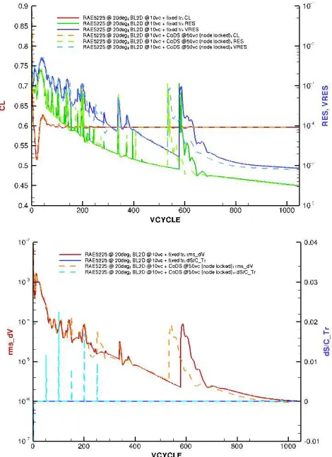
As indicated earlier, the results of interest are the convergence rates of the solutions, and the most interesting case was the RAE5225 section swept at 20°, which consistently required longer to converge than the other cases. The upper plot in Fig. 4 illustrates the convergence rates of lift, and – on the secondary abscissa – the decay of the inviscid (RES) and viscous (VRES) VGK residuals, for the fixed transition ‘stdb’ and the ‘lam1’ strategies, solid and dashed lines respectively. The lower plot presents additional convergence information from Callisto: the r.m.s. change in transpiration rate (the boundary condition applied to the inviscid solver) which more or less matches the VRES curve on the upper plot, and – on the secondary abscissa – the overall movement in transition position.

Generally speaking, the transition updates do not become apparent in the convergence plots

Fig. 4: RAE5225 swept at 20°; results for ‘stdb’ strategy (solid lines) compared with ‘lam1’ strategy (dashed).

until the VGK viscous residuals drop below 10-3, although there are large spikes late in the convergence plots of a number of analyses which are nothing to do with the transition analysis. Where transition position is re-calculated but left unchanged (there are tolerances limiting minute adjustments to transition position), there is no visible trace in the convergence plot.

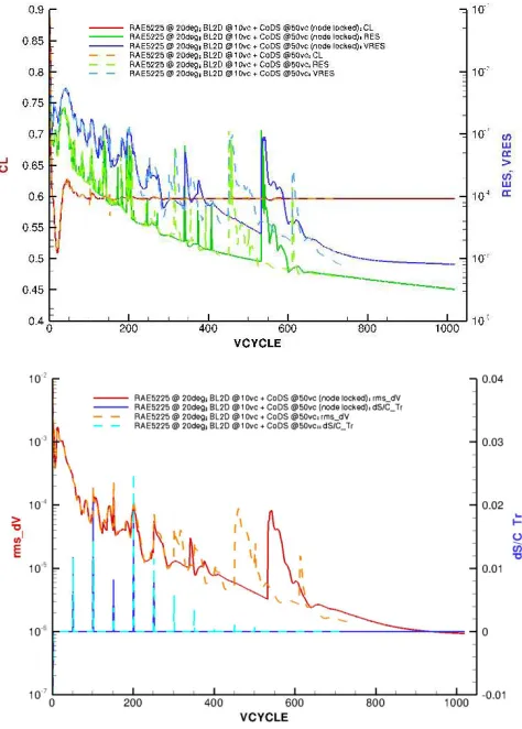
Fig. 5 shows how removing the node-locking constraint on transition location results in an increased number of transition movements, but an overall more rapid convergence. This is also evident from the upper surface transition history presented in Table 3 overleaf, as is the beneficial effect of increasing the under-relaxation factor on transition movement from 0.5 (‘lam1a’) to 0.9 (‘lam5’).

C J ATKIN

Fig. 5: RAE5225 swept at 20°; results for ‘lam1’ strategy (solid lines) compared with ‘lam1a’ strategy (dashed).

VCYCLE ‘lam1’ ‘lam1a’ ‘lam5’

1 x/c = 1.51% x/c = 1.51% x/c = 1.51% 5 x/c = 1.51% x/c = 1.51% x/c = 2.02% 51 x/c = 2.60% x/c = 2.60% x/c = 3.25% 101 x/c = 4.78% x/c = 3.98% x/c = 6.60% 151 x/c = 3.98% x/c = 3.61% x/c = 3.56% 201 x/c = 5.65% x/c = 6.05% x/c = 8.01% 251 x/c = 6.60% x/c = 7.18% x/c = 8.68% 301 x/c = 6.60% x/c = 7.74% x/c = 8.45% 351 x/c = 6.60% x/c = 8.09% unchanged 401 x/c = 6.60% x/c = 8.18% unchanged 451 x/c = 6.60% x/c = 8.32% unchanged 501 x/c = 6.60% x/c = 8.39% unchanged

551 x/c = 6.60% unchanged unchanged

601 x/c = 6.60% unchanged unchanged

651 x/c = 6.60% unchanged unchanged

701 x/c = 6.60% unchanged unchanged

Table 3: RAE5225 @ 20°; upper surface transition history, ‘lam1’, ‘lam1a’ and ‘lam5’ strategies.

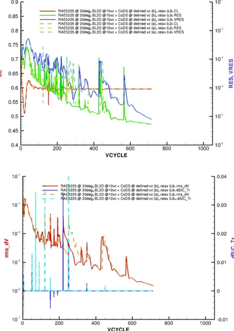
Fig. 6: RAE5225 @ 20°; results for ‘lam5’ strategy (solid lines) compared with ‘lam4’ strategy (dashed).

Fig. 7: RAE5225 @ 20°; results for ‘lam5’ strategy (solid lines) compared with ‘lam6’ strategy (dashed).

VC x/c (tr) VC x/c (tr) VC x/c (tr)

1 1.51% 81 7.42% 181 3.52%

5 2.02% 101 5.19% 201 8.02%

21 2.60% 121 3.89% 221 8.64%

41 3.17% 141 3.59% 241 8.41%

61 4.46% 161 3.27% 261 on unchanged

Table 4: RAE5225 @ 20°; upper surface transition history for ‘lam4’ strategy.

that the ‘lam4’ strategy (transition updated every 20 viscous cycles) does not improve the overall convergence rate and is therefore inefficient. However transition location does converge earlier in the solution, albeit with more updates, than for the ‘lam6’ strategy (transition updated every 100 viscous cycles), Fig. 7. These trends are confirmed by the upper surface transition histories presented in Table 4 and Table 5.

In an attempt to find the middle ground between ‘lam4’, where transition was converged by 220 viscous cycles but at significant

computational cost, and ‘lam6’ where transition was still changing after 450 viscous cycles, two new strategies ‘lam7’ and ‘lam8’ were devised in which a basic 50-cycle transition interval was augmented by a number of more frequent

VC ‘lam6’ x/c (tr)

VC ‘lam7’ x/c (tr)

VC ‘lam8’ x/c (tr)

1 1.51% 1 1.51% 1 1.51%

5 2.02% 5 2.02% 5 2.02%

51 3.25% 51 3.25% 51 3.25%

71 6.60%

91 7.60%

121 3.99%

151 unchanged 151 3.53% 151 unchanged

171 3.39% 191 3.24% 221 6.60%

251 6.60% 251 8.08% 251 8.17%

351 8.21% 351 8.24% 351 8.44%

451 8.44% 451 8.44% 451 unchanged

551 unchanged 551 unchanged 551 unchanged 651 unchanged

Table 5: RAE5225 @ 20°; upper surface transition history for ‘lam6’, ‘lam7’ & ‘lam8’ strategies.

C J ATKIN

analyses either just before (‘lam7’) or just after (‘lam8’) the point at which overall wing lift appeared to be converging, at around 150 viscous cycles. Convergence plots for the two schemes are presented in Fig. 8 and transition updates tabulated in Table 5. Overall it appears, more clearly from Table 5 than from Fig. 8, that adding extra transition updates before the pressure distribution was converged (‘lam7’) delivered no benefits compared to ‘lam6’, while the ‘lam8’ approach resulted in transition convergence some 100 viscous cycles earlier than ‘lam6’, although still 100 viscous cycles later than the high-resolution ‘lam4’ approach.

6 Conclusions

An extensive investigation has been carried out into the convergence of transition loci during the viscous-coupled analysis of three well-known transonic wing sections in 2D and infinite-swept configurations. A number of challenges to solution convergence were diagnosed and addressed.

Once the operational fixes described in section 4 were implemented, good convergence of transition loci was observed and a number of trends emerged:

1. Frequent transition updates (every 20 viscous cycles) delayed the convergence of both the inviscid and viscous residuals.

2. Infrequent transition updates (every 100 or even 50 viscous cycles) often resulted in the residuals converging before the next transition update, even if the transition locus itself was still unconverged.

3. Best practice would appear to be to run a series of four or five transition updates at frequent intervals (20 viscous cycles for the CVGK case) immediately after the convergence of the lift coefficient (and therefore the pressure distribution), followed by longer intervals to allow adjustments arising from more subtle changes in the pressure distribution over a longer period of time.

4. Frequent transition calculations prior to the convergence of the overall lift coefficient did not accelerate the overall convergence of the transition locus.

There is no reason apparent from this study why points (3) and (4) above should not be equally applicable to higher-order, e.g. RANS, methods incorporating transition modelling.

Point (3) is perhaps an inevitable conclusion for the current selection of test cases, given that the transition locus is very sensitive to the pressure distribution (particularly for the RAE5225 @ 20° case highlighted in this paper). In the event that the converse were true – that is, that the pressure distributions were very sensitive to the transition locus, for example in a high-lift configuration – then one might expect this recommendation, and point (4) above, to be less appropriate.

Acknowledgement

This study was supported by QinetiQ Ltd under contract number 3000074262.

References

[1] M. Arthur and C. Atkin. “Transition modelling for viscous flow prediction,” AIAA 36th Fluid Dynamics

Conference, San Francisco, 2006.

[2] M. Milne and M. Arthur. “Evaluation of bespoke and commercial CFD methods for a UCAV

configuration,” AIAA 36th Fluid Dynamics

Conference, San Francisco, 2006.

[3] N. Krimmelbein and A. Krumbein. “Automatic Transition Prediction for Three-Dimensional

Configurations with Focus on Industrial Application,”

J. Aircraft, Vol. 48, No. 6, 2011.

[4] A. Probst, R. Radespiel and U. Rist. “Linear-Stability-Based Transition Modeling for Aerodynamic Flow simulations with a Near-Wall Reynolds-Stess Model,”

AIAA Journal, Vol. 50, No. 2, 2012.

[5] C. Seyfert and A. Krumbein. “Evaluation of a Correlation-Based Transition Model and Comparison with the eN Method,” J. Aircraft, Vol. 49, No. 6, 2012.

[6] J. Green, D. Weeks and J. Brooman. “Prediction of turbulent boundary layers and wakes in compressible flow by lag-entrainment method,” ARC R&M, 1973.

[7] R. Lock and B. Williams. “Viscous and inviscid interactions in external aerodynamics,” Progress in

Aerospace Science, vol. 24, 1987.

[8] P. Garabedian and D. Korn. “Analysis of transonic aerofoil,” Communications on Pure and Applied

Mathematics, vol. 24, 1971.

two-dimensional pressure distributions.,” NPL Aero Report no. 1028, 1962.

[10] P. Ashill, R. Wood and D. Weeks. “An improved, semi-inverse method of the viscous Garabedian and Korn method (VGK),” RAE Technical Report 87002, 1987.

[11] C. J. Atkin and E. R. Gowree. “Recent Development to the Viscous Garabedian and Korn Method,” 28th

International Congress of the Aeronautical Sciences,

Brisbane, 2012.

[12] H. P. Horton and H. W. Stock. “Computation of Compressible Boundary Layers on swept, tapered wings,” J Aircraft, Vol. 32 no. 6, 1995.

[13] C. J. Atkin. “New Aerodynamic Approach to Suction System Design,” DragNet European Drag Reduction

Conference, Potsdam, June 2000.

Contact Author Email Address

[email protected]

Copyright Statement