1
A comparative investigation of the combined effects of
pre-processing, wavelength selection and regression methods
on near infrared calibration model performance
Jian Wan1, Yi-Chieh Chen2, A. Julian Morris2a, Suresh N. Thennadil3*
1School of Marine Science and Engineering, Plymouth University, Plymouth PL4 8AA, UK 2Department of Chemical and Process Engineering, University of Strathclyde, Glasgow G1 1XJ, UK
2aCentre for Process Analytics and Control Technology, University of Strathclyde, Glasgow 3* School of Engineering and Information Technology
Charles Darwin University, Darwin, Northern Territory 0909, Australia E-mail: [email protected] (S.N.Thennadil), Tel: +61 8 89466564
This is a peer-reviewed, accepted author manuscript of the following research output: Wan, J., Chen, Y-C., Morris, A. J., & Thennadil, S. N. (2017). A comparative investigation of the combined effects of pre-processing, wavelength selection, and
2
Abstract
Near infrared (NIR) spectroscopy is being widely used in various fields ranging from pharmaceutics to food industry for analysing chemical and physical properties of the substances concerned. Its advantages over other analytical techniques include available physical interpretation of spectral data, non-destructive nature and high speed of measurements, and little or no need for sample preparation. The successful application of NIR spectroscopy relies on three main aspects: pre-processing of spectral data to eliminate nonlinear variations due to temperature, light scattering effects and many others; selection of those wavelengths that contribute useful information; identification of suitable calibration models using linear/nonlinear regression. Several methods have been developed for each of these three aspects and many comparative studies of different methods exist for an individual aspect or some combinations. However, there is still lack of comparative studies for the interactions among these three aspects, which can shed light on what role each aspect plays in the calibration and how to combine various methods of each aspect together to obtain the best calibration model. This paper aims to provide such a comparative study based on four benchmark data sets using three typical pre-processing methods namely, orthogonal signal correction (OSC), extended multiplicative signal correction (EMSC) and optical path-length estimation and correction (OPLEC), two existing wavelength selection methods namely, stepwise forward selection (SFS) and Genetic algorithm optimization combined with partial least squares regression for spectral data (GAPLSSP), four popular regression methods namely, partial least squares (PLS), least absolute shrinkage and selection operator (LASSO), least squares support vector machine (LS-SVM) and Gaussian process regression (GPR). The comparative study indicates that, in general, pre-processing of spectral data can play a significant role in the calibration while wavelength selection plays a marginal role and the combination of certain pre-processing, wavelength selection and nonlinear regression methods can achieve superior performance over traditional linear regression-based calibration.
3 1. Introduction
Near infrared (NIR) spectroscopy measures overtones and combination tones of the fundamental molecular vibrations in the region of about 780-2526 nm or 12820-3959 cm-1 [1].
As a wide range of products contain infrared-active molecules, NIR spectroscopy can be used in many fields such as pharmaceutical, petrochemical, biological, biomedical and agricultural sectors to provide chemical and physical information of the substances concerned [2]. It has also been increasingly adopted as the favoured analytical tool in these fields for its advantages over other analytical tools. These advantages include available physical interpretation of spectral data, non-destructive nature and high speed of measurements, and little or no need for sample preparation [3].
The NIR spectra for a sample are usually a series of intensity values for hundreds of wavelengths. According to Beer-Lambert’s law, the absorbance spectra are ideally linear in the properties of the analyte such as its concentration. However, such a linear relationship generally does not exist in practice as many external factors such as light scattering effects and varying temperatures introduce nonlinear variations into the spectral data [4, 5]. Therefore the raw spectral data should be pre-processed to remove such nonlinear variations and then linear regression methods can be used for the calibration to link the pre-processed spectra and the concerned properties. Pre-processing of NIR spectra has thus become an integral part of calibration and many pre-processing methods have been proposed in the literature. An excellent review of the most common pre-processing techniques for NIR spectra can be found in [6].
4
model as a result of the added penalty. These spectral variables with zero coefficients are deemed to be redundant as they do not contribute information in the calibration model.
Alternatively, nonlinear regression methods can be used to model the non-linearity in the spectral data. For example, artificial neural networks were applied for spectroscopic calibration in [4, 10-12]; least squares support vector machines (LS-SVM) were used for multivariate calibration to deal with ill-posed problems [13]; Gaussian process regression (GPR) was used for multivariate spectroscopic calibration in [14]. There are other nonlinear regression methods that are applied for NIR spectra calibration and it is worthwhile to note that the spectra data used for nonlinear regression is often pre-processed as in the linear regression-based calibrations.
In case of existing collinearity and redundancy among the raw or the pre-processed spectral data, the selection of useful wavelengths or the elimination of uninformative wavelengths before regression can also play a positive role to obtain a reliable regression model regardless of linear and nonlinear regression. The aforementioned regularized regression methods can be regarded as an integration of wavelength selection and regression because of their sparse solution. The importance of wavelength selection in NIR spectroscopy was summarized in [3] from various bases and the paper also gave an extensive review on existing wavelength selection methods. The benefits of wavelength selection for linear/nonlinear calibrations can be found in benchmark studies [2, 8].
5
sets. However, there is still lack of comparative studies on the interactions among these three aspects of pre-processing, wavelength selection and linear/nonlinear regression. Such benchmark studies can shed light on what role each aspect plays in the calibration and how to combine various methods of each aspect together to obtain the best calibration model.
Inspired by the comparative study in [4], where the interactions between pre-processing and linear/nonlinear regression methods were examined, this paper includes wavelength selection methods into the comparative study as well and explores the interactions among all three aspects of pre-processing, wavelength selection and linear/nonlinear regression for NIR spectra calibration. A further contribution of this paper is that the comparison of the methods are carried out using a dataset in which the particle size and concentration varies significantly thus including significant nonlinear variations in the spectra due to appreciable variations in light scattering effects. This allowed the analysis of two types of situations: One where the analyte of interest is a purely absorbing species in a sample containing particles and the second where the analyte of interest is the particulate component i.e. a component which absorbs and scatters light.
The paper is organized as follows: first, techniques for pre-processing, wavelength selection, linear/nonlinear regression and cross validation are briefly introduced in Section 2; the two data sets as well as the approaches and the software used for the benchmark studies are described in Section 3; Section 4 details the performance evaluation and the corresponding observations on the two benchmark studies, respectively; finally, some conclusions are drawn in Section 5.
2. Techniques for calibration
As the combination options for various pre-processing, wavelength selection and linear/nonlinear regression methods are enormous, it is prohibitive to compare them all and thus only a limited number of methods are selected from each aspect to conduct the comparative study. The methods selected for the comparative study are briefly introduced in the following subsections and these selected methods are deemed to be representative or the most promising ones.
The notations used in this section are as follows: 𝑥𝑖,𝑗 denotes the raw spectra for the 𝑖𝑡ℎ sample
at the 𝑗𝑡ℎ wavelength; 𝑿
6
sample and the corresponding response variable of the 𝑖𝑡ℎ sample, respectively; 𝑿 is a matrix of 𝐼 × 𝐽 for the spectral data of all samples and 𝒚 is the corresponding column vector for the response variable of all samples where 𝐼 is the number of samples and 𝐽 is the number of spectral variables.
2.1 Pre-processing
Three typical pre-processing methods are selected for the comparative study: orthogonal signal correction (OSC), extended multiplicative signal correction (EMSC) and optical path-length estimation and correction (OPLEC). EMSC was chosen since several studies indicate that it generally works better (or at least as well as) than other standard pre-processing methods such as standard normal variate (SNV) and `multiplicative scatter correction (MSC). OPLEC was chosen since it is a relatively new technique, which has shown promising results in a limited number of studies indicating that it could outperform widely used pre-processing methods. OSC was chosen as a possible option since it works on different principles from the standard scatter correction methods and could potentially be a good pre-processing alternative.
OSC is derived from the ordinary PLS algorithm with the aim of removing bilinear components from 𝑿 which are orthogonal to 𝒚 [16]. The method was applied to enhance NIR calibration of wort fermentability [17]. There are other variants of OSC algorithms proposed in the literature with successful applications therein [18-20].
EMSC is an extension of multiplicative signal correction (MSC) by considering wavelength-dependent spectral variations: 𝑿𝑖 = 𝑎𝑖+ 𝑏𝑖𝑿𝑖𝑐ℎ𝑒𝑚+ 𝑑𝑖𝝀+𝑒𝑖𝝀2, where 𝑿𝑖𝑐ℎ𝑒𝑚 is the theoretical spectra; 𝝀is the wavelength vector; the coefficients 𝑎𝑖, 𝑏𝑖, 𝑑𝑖 and 𝑒𝑖 can be estimated by least squares regression of 𝑿𝑖 to 𝑿𝑖𝑐ℎ𝑒𝑚. As 𝑿𝑖𝑐ℎ𝑒𝑚 is seldom known in practice, it is usually replaced by the mean spectra of 𝑿 [21]. Once the coefficients are estimated, the corrected spectra of 𝑿𝑖 is given by 𝑿̂𝑖 = ( 𝑿𝑖 − 𝑎𝑖−𝑑𝑖𝝀 − 𝑒𝑖𝝀2) ∕ 𝑏
𝑖.
7
projected spectra for the multiplicative variations. OPLEC can be regarded as an extension of EMSC with no need to estimate 𝑎𝑖, 𝑑𝑖 and 𝑒𝑖 because of the projection at the first step.
2.2 Wavelength selection
Two existing wavelength selection algorithms called stepwise forward selection (SFS) and Genetic algorithm optimization combined with partial least squares regression for spectral data (GAPLSSP) are adopted for the comparative study.
SFS is a sequential feature selection technique designed specifically for least-squares fitting and it makes use of optimizations that are only possible with least-squares criteria. Unlike generalized sequential feature selection, SFS may remove features that have been added or add features that have been removed [23]. Whether to retain a variable in the model is based on the level of significance assumed for inclusion and exclusion of the variable from the model. SFS can reduce the dimensionality of NIR spectra data by selecting an influential subset of the original wavelengths.
GAPLSSP combines the advantage of genetic algorithms (GA) for optimisation and the convenience of PLS for performance evaluation [24, 25]. It returns an optimal subset of the original wavelengths that provides the enhanced predictive capability. GAPLSSP can explore fairly well the space of all possible subsets from the original wavelengths in a large but reasonable time [3].
2.3 Linear/nonlinear regression
Two linear regression methods called PLS and least absolute shrinkage and selection operator (LASSO) and two nonlinear regression methods called LS-SVM and GPR are adopted for the comparative study.
PLS identifies the linear relationship from 𝑿 to 𝒚 through two related projections:
𝑿 = 𝑻𝑷′, (1)
𝒚 = 𝑼𝑸′, (2)
8
𝒚 = 𝑿𝑽𝑩𝑸′. (3)
LASSO is an extension of MLR by adding a ℓ1-norm penalty item for the cost function to obtain a sparse solution:
𝐽(𝑾) = 12‖𝒚 − 𝑿𝑾‖2+‖𝑾‖1, (4)
where𝑾 is the regression coefficients; ‖𝑾‖1 = ∑ |𝑤𝑗 𝑗| is the ℓ1-norm penalty on 𝑾, which renders some 𝑤𝑗=0 to generate a sparse solution; is the tuning parameter.
LS-SVM is an extension of support vector machine (SVM) and it is also a regularized regression method which penalizes the square values of the weights [13]. The kernel-based LS-SVM is adopted in this study to deal with nonlinearity in the spectral data and the LS-LS-SVM model can be expressed as follows:
𝒚(𝑿) = ∑𝑁 𝛼𝑖𝜅(𝑿, 𝑿𝑖) + 𝑏
𝑖=1 , (5) where 𝛼𝑖 is the Lagrange multiplier; 𝜅(𝑿, 𝑿𝑖) is the kernel function; and 𝑏 is the bias value. The radial basis function (RBF) kernel is used in this paper and the function can be expressed as follows:
𝜅(𝑿, 𝑿𝑖) = exp(−‖𝑿 − 𝑿𝑖‖2⁄ ), (6) 𝜎2 where 𝜎2 is the bandwidth and it implicitly defines the nonlinear mapping from input space to some high-dimensional feature space [8].
GPR is a probabilistic non-parametric modelling technique assuming that the joint distribution over any finite set of fixed test points is a multivariate Gaussian [14, 26]. The Gaussian process is fully specified by the mean function and the covariance function of this joint Gaussian distribution. The mean function is often assumed to be zero. The parameters 𝛳 for the covariance function can be optimized to maximize the conditional probability 𝑝(𝛳|(𝑿, 𝛳)) using the training data. According to Bayes’ rule, the related 𝒚 for a new sample can then be predicted by extending the joint distribution with the optimized covariance function.
2.4 Cross validation
9
The evaluation can be based on the root-mean-square error of prediction (RMSEP) for the test set, which is calculated as follows:
𝐑𝐌𝐒𝐄𝐏 = √∑𝑛𝑖=1(𝑦𝑖−𝑦̂𝑖)2
𝑛 (7)
where 𝑛 is the number of test samples; 𝑦𝑖 and 𝑦̂𝑖 are the reference and the predicted values of the 𝑖th sample, respectively.
As the test set is just a subset of all the available samples, RMSEP can be biased for different subsets formed from the available samples. The bias can be considerably large for a specific subset, especially for the case that the size of the whole available samples is relatively small. In order to reduce such kind of bias so as to evaluate the performance of the identified regression models in a statistically robust and reliable way, the simulation method used in [4, 27] is adopted here, which is to randomly divide the whole data set into training and testing parts multiple times and then to compute an average RMSEP (ARMSEP) for all the divisions. Assume that the number of the divisions is 𝑀 and the ratio for the division is 𝑟 while 𝑟 ∙ 𝑁 is the number of samples for training and 𝑁 is the total number of all available samples, the
ARMSEP can be computed as follows:
𝐀𝐑𝐌𝐒𝐄𝐏 = ∑
√∑(1−𝑟)∙𝑁𝑖=1 (𝑦𝑖𝑗−𝑦̂𝑖𝑗)2 (1−𝑟)∙𝑁 𝑀
𝑗=1
𝑀 (8)
where 𝑦𝑖𝑗 and 𝑦̂𝑖𝑗 are the reference and the predicted values of the 𝑖th sample for the 𝑗th division.
10
There are two sources contributing to the uncertainties in the estimated RMSEP namely, the number of latent variables (LVs) chosen and the particular division of the dataset into calibration and validation set. If the optimal number of LVs specific to the division is chosen each time and the ARMSEP calculated we would expect that the uncertainty in the estimated ARMSEP would be less than or equal to the uncertainty in the estimates calculated based on fixing the number of LVs according to the first division. Therefore the uncertainty of estimates (error bars) obtained by fixing the LVs according to the first division are conservative estimates. Since the study is about comparing the performances of different methods and judging whether the results from different methods are significantly different, the conservative values are at least as good for this purpose as using ARMSEP values and corresponding error bars calculated from models built with optimal LVs chosen for each division. Another point to consider is that the optimal number of LVs is not always evident since two or more adjacent LVs may be equally likely candidates and some subjectivity is involved in the choice. Since we expect the optimal number to vary by one or two LVs for all the divisions, they could very well be within the level of uncertainty in the choice based on the first division. This reasoning was testing by choosing the latent variables using 3 different divisions and the results and conclusions were consistent with those reported here.
3. Benchmark studies
3.1 Data sets
Four NIR data sets with varying characteristics are used for the benchmark studies. The first data set is the NIR analysis of pharmaceutical tablets and it is available at http://www.models.life.ku.dk/Tablets. The data set consists of NIR measurements of 310 samples with 404 wavelengths ranging from 952nm to 1352nm. The NIR measurements are used to determine the relative active substance (escitalopram) content of the tablets with a range from 4.61% to 9.79% in weight percentage [29]. As indicated in Ref 28, a broad 2nd overtone
11
microcrystalline cellulose constituting roughly about 80%. The coated table contained in addition, a coating material which contained titanium oxide.
This can be considered as a model system for compressed powder mixtures (i.e. tablets) that commonly occur particularly in pharmaceutical industry since it incorporates variations in multiple particulate components such as active ingredient, excipients, coating component and variations in these due to batch-to-batch variations and production scale variations, changes in dosage levels of the active substance. The dataset also included the effect of variations in the tablet thickness and shape. For each cross validation step, 217 samples were randomly selected as the training data for model development while the remaining 93 samples were used for the test set and the process was repeated 𝑀 = 20 times to obtain the ARMSEP value from these 20 random divisions.
The second data set is the NIR measurements of a multicomponent system consisting of water (H2O), deuterium oxide (D2O), ethanol (C2H5OH), and polystyrene particles [30]. The
polystyrene particles in the suspension absorb and scatter light, which adds nonlinear variations into NIR spectra. The purpose of the data set is two folds: one is to directly predict the concentration of polystyrene; the other is to predict the concentration of other solutes with a background of nonlinear variations induced by polystyrene particles. The experiments were designed so that the concentrations of polystyrene and ethanol are uncorrelated with all the other components in the sample. Totally 45 samples were prepared with various concentrations and particle diameters and the NIR measurements consist of 191 wavelengths ranging from 1500nm to 1880nm taken at 2 nm intervals. Specifically, the relative concentration of polystyrene in volume percentage ranges from 0.96% to 4.95% and the relative concentration of ethanol in volume percentage ranges from 2.58% to 13.07% for these 45 samples. In the dataset collected, the polystyrene particle diameter varied from 100nm to 500nm which is the typical size range in emulsion polymerisation processes and also to ensure that the range was sufficient to introduce sufficient non-linearity due to scattering that is typically found in a variety of suspensions. For the cross validation, the samples were also randomly divided into 32 samples for the training set and 13 samples for the test set and the process was repeated 𝑀 = 20 times as well to obtain the ARMSEP value from these 20 random divisions.
The third dataset used in this study is the NIR measurements of corn which is available at
12
consists of 80 samples with 700 wavelengths ranging from 1100nm to 2498nm with an interval of 2nm. The measurements are for the property of protein with a range from 7.654 to 9.711 wt%. For cross validation, 56 samples were randomly selected as the training data for model development while the remaining 24 samples were used for the test set and the process was repeated M=20 times to obtain the ARMSEP value from these 20 random divisions.
The fourth Dataset used in this study is the Visible-NIR measurements of sugarcane which is available from http://www.models.life.ku.dk/nirsugarcanedata, details of which can be found in the paper [31]. Briefly, the dataset consists of 599 samples which are selected at an interval of 3 samples from a total of 1797 available samples with 744 wavelengths ranging from 402nm to 1850nm with an interval of 2nm covering all four process steps together for the simulation study. The measurements of Y have a minimum value of 12.92% and a maximum value of 77.95% in terms of mass percentage. For cross validation, 419 samples were randomly selected as the training data for model development while the remaining 180 samples were used for the test set and the process was repeated 𝑀 = 20 times to obtain the ARMSEP value from these 20 random divisions.
3.2 Approaches
The comparative studies were performed on these two data sets, respectively. Four regression methods, namely, PLS, LASSO, LS-SVM and GPR, are used for each data set. For each regression method, there are twelve calibration approaches based on the existence and the selection of three pre-processing methods of OSC, EMSC and OPLEC and two wavelength selection methods of SFS and GAPLSSP. These twelve calibration approaches are listed in Table 1 and the ARMSEP value of each approach is computed as its performance index. For example, the approach No. 1 means that no pre-processing and no wavelength selection are performed for the calibration; the approach No. 6 means that the pre-processing method of OSC and the wavelength selection method of GAPLSSP are performed for the calibration; and the approach No. 10 means that the pre-processing method of OPLEC is performed and no wavelength selection is performed for the calibration. As each regression method has twelve approaches, the total number of calibration approaches for one data set is forty-eight for the selected four regression methods.
13 Approach
No.
Pre-processing Wavelength selection
OSC EMSC OPLEC SFS GAPLSSP
1 × × × × ×
2 × × × ×
3 × × × ×
4 × × × ×
5 × × ×
6 × × ×
7 × × × ×
8 × × ×
9 × × ×
10 × × × ×
11 × × ×
12 × × ×
3.3 Software
The comparative study was carried out in MATLAB. Specifically, the functions of PLS, cross validation and SFS were performed by the Statistics Toolbox of MATLAB; the function of OSC was performed by the PLS Toolbox from Eigenvector Research, Inc., Wenatchee, WA, USA; the function of OPLEC was from the MATLAB code provided in [5]; the function of
GAPLSSP was performed by the PLS-Genetic Algorithm Toolbox at
14
the pre-processed/wavelength-selected training data sets; and making predictions for the original and the pre-processed/wavelength-selected test data sets using the identified calibration models.
4. Results and discussions
4.1 Pharmaceutical tablets
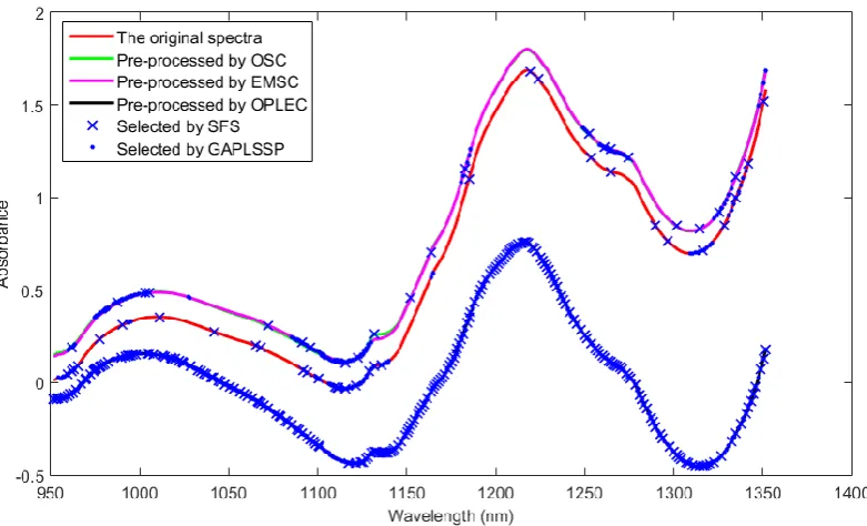
The spectra for 310 pharmaceutical tablets are pre-processed by OSC, EMSC and OPLEC, respectively and these corrected spectra along with the original spectra are shown in Figure 1. It can be seen that the degree of the corrections is different for these three pre-processing methods, where OPLEC has the smallest corrections and EMSC has the most corrections.
The wavelength selection algorithms of SFS and GAPLSSP were performed on the original and the pre-processed spectra to eliminate uninformative wavelengths. Taking the 10th sample in
15 Figure 1 Orginial and pre-processed spectra of pharmaceutical tablet samples.
Figure 2. Pre-processing and wavelength selection for the 10th pharmaceutical tablet sample.
[image:15.595.104.495.396.633.2]16
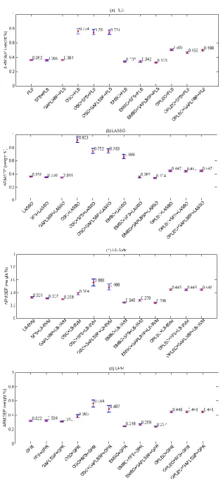
that the nonlinear regression methods of LS-SVM and GPR perform better than the linear regression methods of PLS and LASSO when they are directly applied without pre-processing or wavelength selection.
The impact of pre-processing and wavelength selection on the PLS model performance can be examined by considering Figure 3(a). It can be seen that pre-processing impacts significantly on the performance while wavelength selection only impacts marginally on the performance. The performance has been slightly improved for the cases of GAPLSSP and also for most cases of SFS except the case of EMSC+SFS+PLS. Among the three pre-processing methods OSC has the worst performance leading to the highest level of performance degradation with an
ARMSEP value of 0.76%. The best result among all PLS-based approaches is obtained by combining EMSC and GAPLSSP, which leads to an ARMSEP value of 0.323%.
The impact of pre-processing and wavelength selection on the LASSO model performance can be examined by considering Figure 3(b). Similar to the PLS-based approaches, pre-processing impacts significantly the performance while wavelength selection impacts marginally the performance. The inclusion of wavelength selection generally improves the performance regardless of SFS and GAPLSSP for LASSO-based approaches and the degree of improvement depends on the interactions among the pre-processing and wavelength selection methods. For example, wavelength selection can improve the performance greatly for the pre-processing methods of OSC and EMSC. Similar to the results seen for PLS, the best performance among all LASSO-based approaches is also obtained by combining EMSC and GAPLSSP, which leads to an ARMSEP value of 0.334%.
18
The best performance is still the combination of EMSC and GAPLSSP, which leads to an
ARMSEP value of 0.236%. The impact of pre-processing and wavelength selection on the GPR model performance can be examined by considering Figure 3(d), which is quite similar to the case of LS-SVM with an ARMSEP value of 0.237% for the best performance model.
It should be noted that in LASSO, some regression coefficients turn out to be zero. This results in reduction in wavelengths in addition to the reduction due to the application of SFS or GAPLSSP. For the analysis shown in Figure 3(b), 7 out of 25 wavelengths selected by SFS were set to zero and 13 out of 81 wavelengths selected by GAPLSSP were set to zero. The results suggest that LASSO can reduce about 15%-30% of wavelengths needed for the model.
Based on these observations, for this data set we can conclude that the nonlinear regression methods have superior performance compared to the linear regression methods. EMSC is consistently the most effective pre-processing method and wavelength selection using GAPLSSP can marginally improve the model performance for both linear and nonlinear regression methods.
4.2 Multicomponent suspension
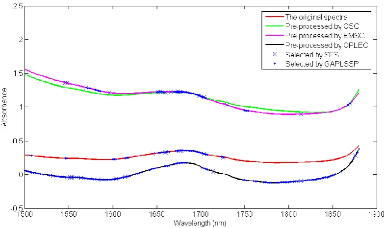
The original and the OSC-corrected, EMSC-corrected and OPLEC-corrected spectra for the multicomponent system are shown in Figure 4. The degree of the corrections is also different for these three pre-processing methods and OSC has the least corrections while EMSC has the most corrections.
The first case study for this data set is to predict the concentration of polystyrene particles. The wavelength selection algorithms of SFS and GAPLSSP are also performed on these four types of spectra to eliminate uninformative wavelengths. Taking the 10th sample in the data set as an
19
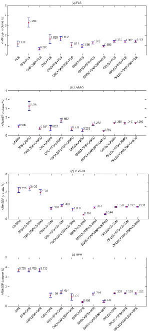
[image:19.595.80.522.176.440.2]The comparisons of PLS, LASSO, LS-SVM and GPR for predicting the concentration of polystyrene particles are shown in Figure 6. For the twelve PLS-based approaches, the number of latent variables is selected to be 7,6,6,7,4,5,6,4,5,4,5 and 4, respectively.
Figure 4 Original and pre-processed spectra of all samples in the polystyrene suspension dataset.
[image:19.595.102.495.499.732.2]21
Figure 6 Comparisons of PLS, LASSO, LS-SVM and GPR for polystyrene particle concentration.
The 95% confidence intervals for ARMSEP are relatively big for this data set due to the small size of the whole data set. For the case of PLS-based approaches, the best performance is obtained by combining EMSC and GAPLSSP with an ARMSEP value of 0.313%. Similarly for LASSO-based approaches, the best performance is also obtained by combining EMSC and GAPLSSP with an ARMSEP value of 0.343%. Unlike the tablet data set where non-linear regression methods performed consistently better than the linear regression methods, the performances of LS-SVM and GPR are not always positive for this data set. Nevertheless, the best performance among all approaches is still obtained by the nonlinear regression method of
LS-SVM with combination of EMSC and GAPLSSP, which leads to an ARMSEP value of
0.254%. Figure 6 also indicates that in general, the pre-processing methods of EMSC and OPLEC perform better than the processing method of OSC. Depending on the pre-processing methods and the regression methods, wavelength selection can play either a positive or a negative role. GAPLSSP tends to work better than SFS in most cases.
The reason underlying the negative impact of SFS for the nonlinear regression methods could be that these wavelength selection methods are basically linear approaches, which are internally designed for linear regression methods. Therefore it is not suggested to use these wavelength selection methods for LS-SVM-based or GPR-based calibrations. It would be worthwhile to develop specific wavelength selection methods for these nonlinear regression methods so as to improve the corresponding calibration performance.
22
23
selected to be 6,4,6,4,3,3,5,3,3,3,4 and 3, respectively. Similar to the tablet dataset, this dataset also indicates further 15-30% additional reduction in wavelengths when used in conjunction with SFS and GAPLSSP.
In this case study, the differences among those approaches with and without pre-processing are relatively large, which demonstrates the significance of pre-processing for alleviating nonlinear effects incurred by the existence of polystyrene particles. Meanwhile, wavelength selection also plays a significant role for this case as the ARMSEP value can be reduced from 1.135% for the case of PLS to 0.628% for the case of PLS+GAPLSSP. So the importance of wavelength selection and pre-processing can be correlated to each other depending on the characteristics of spectral data. EMSC is the best pre-processing method for this case as the lowest ARMSEP
values are obtained with this method for all four regression methods. The best performance is still obtained by the nonlinear regression method of GPR with combination of EMSC, which leads to an ARMSEP value of 0.405%. The study further confirms the potential of nonlinear regression methods as they have the capability to obtain the highest calibration accuracy along with suitable pre-processing and wavelength selection methods.
4.3 Corn data set
The spectra for 80 corn samples are pre-processed by OSC, EMSC and OPLEC, respectively and these corrected spectra along with the original spectra are shown in Figure 8. For this dataset, it can be seen that the corrections made by OSC and EMSC are similar and the reduction in the variance of the dataset is greater compared to OPLEC.
Taking the 10th sample in the data set as an example, the selected wavelengths for the original
24
Figure 8 Original and pre-processed spectra of corn samples.
Figure 9 Pre-processing and wavelength selection for the 10th corn sample.
[image:24.595.99.492.373.622.2]26
Figure10 Comparisons of PLS, LASSO, LS-SVM and GPR for corn samples
It can be seen that when PLS is used, wavelength selection using GAPLSSP can provide a slight improvement in model performance. Wavelength selection does not lead to any noticeable improvement when the other 3 regression methods are used. For PLS pre-processing by EMSC does not lead to an improvement while OSC and OPLEC lead to degradation in model performance. For the other 3 regression methods, all the 3 pre-processing methods degrade model performance. When comparing the results when the regression methods are applied on their own, it is seen that LASSO gives the best model performance while GPR leads to the worst performance. Interestingly, when GPR is used in conjunction with EMSC and GAPLSSP, the performance is as good as that obtained by using GPR. It is noteworthy that similar phenomenon is seen with the polystyrene dataset.
4.4 Sugarcane dataset
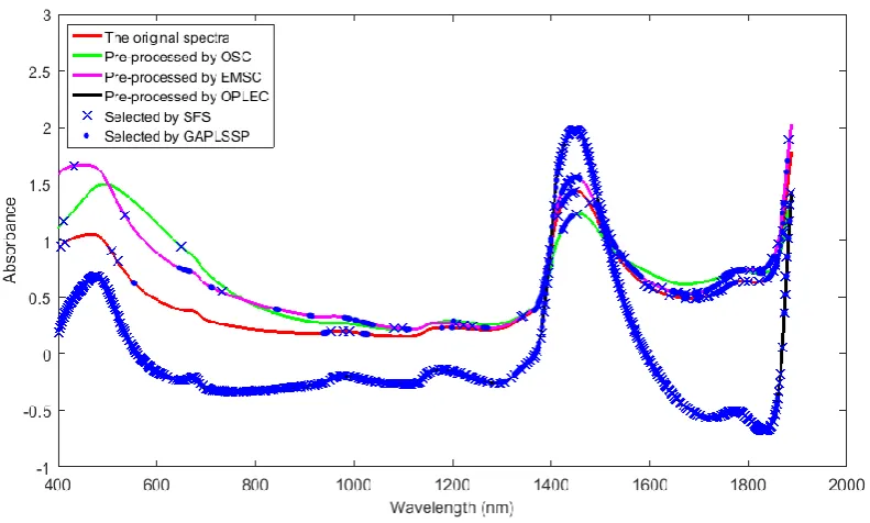
[image:26.595.82.514.401.668.2]The spectra in the dataset were pre-processed by OSC, EMSC and OPLEC, respectively and these corrected spectra along with the original spectra are shown in Figure 11.
Figure 11. Original and pre-processed spectra of sugarcane process samples.
27
[image:27.595.100.496.215.453.2]the data set as an example, the selected wavelengths for the original spectra, the OSC-corrected spectra, the EMSC-corrected spectra and the OPLEC-corrected spectra are shown in Figure 2, where the number of selected wavelengths for the original spectra is 41 by SFS and 90 by GAPLSSP; the number of selected wavelengths for the OSC-corrected spectra is 5 by SFS and 34 by GAPLSSP; the number of selected wavelengths for the EMSC-corrected spectra is 37 by SFS and 194 by GAPLSSP; the number of selected wavelengths for the OPLEC-corrected spectra is 429 by SFS and 370 by GAPLSSP.
Figure 12. Pre-processing and wavelength selection for the 10th sugar sample
The comparisons of PLS, LASSO, LS-SVM and GPR for the calibration are shown in Figure 12, where the ARMSEP value for each approach is plotted by a dot and the vertical bar corresponds to the 95% confidence interval for ARMSEP. The number of latent variables for PLS-based calibrations was selected to be 4, 4, 4, 6, 4, 3, 4, 4, 3, 5, 5 and 5 for the corresponding twelve approaches, respectively.
29
Figure 13 Comparisons of PLS, LASSO, LS-SVM and GPR for sugarcane process samples.
5. Conclusions
Using four benchmark data sets, this comparative study considered various combinations of the three main aspects for NIR spectra calibration and demonstrated their interactions in terms of the calibration performance. The pre-processing methods considered were OSC, EMSC and OPLEC; the wavelength selection methods were SFS and GAPLSSP; and the regression methods considered were PLS, LASSO, LS-SVM and GPR. The comparison was based on a rigorous cross-validation procedure where the data set was randomly divided into two groups and the process was repeated multiple times to obtain an average prediction error as the performance index.
The comparative study has confirmed that in general pre-processing plays a significant role while the wavelength selection plays a marginal role in NIR spectra calibrations. The selection of a suitable pre-processing method can significantly impact the calibration. In the case of non-linear methods, GPR in general performs worse than LV-SVM. However, when EMSC and wavelength selection are used in combination with GPR a large amount of improvement is obtained which can outperform LV-SVM and the linear methods. While it appears that in cases where high degree of nonlinearity in the spectral responses exists, nonlinear regression methods can be advantageous, the popular PLS-based calibration approaches can also achieve a reasonably good performance. Existing wavelength selection methods are mainly designed for linear regression methods and there is potential to obtain better performance if novel wavelength selection methods specifically for nonlinear regression methods can be developed.
Acknowledgement
This project has received funding from the European Union’s Seventh Framework Programme for research, technological development and demonstration under grant agreement no 613665.
References
[1] G. Reich, "Near-infrared spectroscopy and imaging: Basic principles and pharmaceutical applications," Advanced Drug Delivery Reviews, vol. 57, pp. 1109-1143, 6/15/ 2005. [2] R. M. Balabin and S. V. Smirnov, "Variable selection in near-infrared spectroscopy:
Benchmarking of feature selection methods on biodiesel data," Analytica Chimica Acta, vol. 692, pp. 63-72, 4/29/ 2011.
30 [4] K. Wang, G. C. Chi, R. Lau, and T. Chen, "Multivariate Calibration of Near Infrared
Spectroscopy in the Presence of Light Scattering Effect: A Comparative Study," Analytical
Letters, vol. 44, pp. 824-836, 2011.
[5] Z.-P. Chen and J. Morris, "Improving the linearity of spectroscopic data subjected to fluctuations in external variables by the extended loading space standardization," Analyst, vol. 133, pp. 914-922, 2008.
[6] Å. Rinnan, F. v. d. Berg, and S. B. Engelsen, "Review of the most common pre-processing techniques for near-infrared spectra," TrAC Trends in Analytical Chemistry, vol. 28, pp. 1201-1222, 11// 2009.
[7] D. M. Haaland and E. V. Thomas, "Partial least-squares methods for spectral analyses. 1. Relation to other quantitative calibration methods and the extraction of qualitative information," Analytical Chemistry, vol. 60, pp. 1193-1202, 1988/06/01 1988.
[8] F. Liu, Y. Jiang, and Y. He, "Variable selection in visible/near infrared spectra for linear and nonlinear calibrations: A case study to determine soluble solids content of beer," Analytica
Chimica Acta, vol. 635, pp. 45-52, 3/2/ 2009.
[9] J. H. Kalivas, "Overview of two-norm (L2) and one-norm (L1) Tikhonov regularization variants for full wavelength or sparse spectral multivariate calibration models or maintenance,"
Journal of Chemometrics, vol. 26, pp. 218-230, 2012.
[10] J. R. Long, V. G. Gregoriou, and P. J. Gemperline, "Spectroscopic calibration and quantitation using artificial neural networks," Analytical Chemistry, vol. 62, pp. 1791-1797, 1990/09/01 1990.
[11] H. H. Thodberg, "A review of Bayesian neural networks with an application to near infrared spectroscopy," Neural Networks, IEEE Transactions on, vol. 7, pp. 56-72, 1996.
[12] R. M. Balabin, R. Z. Safieva, and E. I. Lomakina, "Comparison of linear and nonlinear calibration models based on near infrared (NIR) spectroscopy data for gasoline properties prediction," Chemometrics and Intelligent Laboratory Systems, vol. 88, pp. 183-188, 9/15/ 2007.
[13] U. Thissen, B. Üstün, W. J. Melssen, and L. M. C. Buydens, "Multivariate Calibration with Least-Squares Support Vector Machines," Analytical Chemistry, vol. 76, pp. 3099-3105, 2004/06/01 2004.
[14] T. Chen, J. Morris, and E. Martin, "Gaussian process regression for multivariate spectroscopic calibration," Chemometrics and Intelligent Laboratory Systems, vol. 87, pp. 59-71, 5/15/ 2007.
[15] W. Ni, L. Nørgaard, and M. Mørup, "Non-linear calibration models for near infrared spectroscopy," Analytica Chimica Acta, vol. 813, pp. 1-14, 2/27/ 2014.
[16] S. Wold, H. Antti, F. Lindgren, and J. Öhman, "Orthogonal signal correction of near-infrared spectra," Chemometrics and Intelligent Laboratory Systems, vol. 44, pp. 175-185, 12/14/ 1998.
[17] E. J. Samp, D. Sedin, and A. Foster, "Enhanced NIR Calibration for Wort Fermentability Using Orthogonal Signal Correction," Journal of the Institute of Brewing, vol. 109, pp. 16-26, 2003. [18] T. Fearn, "On orthogonal signal correction," Chemometrics and Intelligent Laboratory
Systems, vol. 50, pp. 47-52, 1/4/ 2000.
[19] J. A. Westerhuis, S. de Jong, and A. K. Smilde, "Direct orthogonal signal correction,"
Chemometrics and Intelligent Laboratory Systems, vol. 56, pp. 13-25, 4/16/ 2001.
[20] B. Li, A. J. Morris, and E. B. Martin, "Orthogonal signal correction: algorithmic aspects and properties," Journal of Chemometrics, vol. 16, pp. 556-561, 2002.
[21] N. K. Afseth and A. Kohler, "Extended multiplicative signal correction in vibrational
spectroscopy, a tutorial," Chemometrics and Intelligent Laboratory Systems, vol. 117, pp. 92-99, 8/1/ 2012.
[22] Z.-P. Chen, J. Morris, and E. Martin, "Extracting Chemical Information from Spectral Data with Multiplicative Light Scattering Effects by Optical Path-Length Estimation and Correction,"
31 [23] L. Xu and W.-J. Zhang, "Comparison of different methods for variable selection," Analytica
Chimica Acta, vol. 446, pp. 475-481, 11/19/ 2001.
[24] R. Leardi, "Application of genetic algorithm–PLS for feature selection in spectral data sets,"
Journal of Chemometrics, vol. 14, pp. 643-655, 2000.
[25] R. Leardi and A. Lupiáñez González, "Genetic algorithms applied to feature selection in PLS regression: how and when to use them," Chemometrics and Intelligent Laboratory Systems, vol. 41, pp. 195-207, 7/27/ 1998.
[26] M. Ebden, "Gaussian processes for regression: a quick introduction. Technical report: http://www.robots.ox.ac.uk/˜mebden/reports/GPtutorial.pdf.," 2008.
[27] W. Jian, S. Pampuri, P. G. O'Hara, A. B. Johnston, and S. McLoone, "On regression methods for virtual metrology in semiconductor manufacturing," in Irish Signals & Systems Conference 2014 and 2014 China-Ireland International Conference on Information and Communications
Technologies (ISSC 2014/CIICT 2014). 25th IET, 2014, pp. 380-385.
[28] D. Lee, W. Lee, Y. Lee, and Y. Pawitan, "Sparse partial least-squares regression and its applications to high-throughput data analysis," Chemometrics and Intelligent Laboratory
Systems, vol. 109, pp. 1-8, Nov 2011.
[29] M. Dyrby, S. B. Engelsen, L. Nørgaard, M. Bruhn, and L. Lundsberg-Nielsen, "Chemometric Quantitation of the Active Substance (Containing C≡N) in a Pharmaceutical Tablet Using Near-Infrared (NIR) Transmittance and NIR FT-Raman Spectra," Applied Spectroscopy, vol. 56, pp. 579-585, 2002/05/01 2002.
[30] R. Steponavičius and S. N. Thennadil, "Extraction of Chemical Information of Suspensions Using Radiative Transfer Theory To Remove Multiple Scattering Effects: Application to a Model Multicomponent System," Analytical Chemistry, vol. 83, pp. 1931-1937, 2011/03/15 2011.
[31] R. Tange, M. Rasmusson, E. Taira, and R. Bro, "Application of support vector regression for simultaneous modelling of near infrared spectra from multiple process steps," Journal of