A numerical investigation of the squat and resistance of ships advancing through a canal using CFD

A numerical investigation of the squat and

resistance of ships advancing through a canal

using CFD

Tahsin Tezdogan

University of Strathclyde

Department of Naval Architecture, Ocean and Marine Engineering,

100 Montrose Street, Glasgow, G4 0LZ, UK

tahsin.tezdogan@strath.ac.uk

Phone: +44(0)1415484912, Fax: + 44(0)1415522879

Atilla Incecik

University of Strathclyde

Department of Naval Architecture, Ocean and Marine Engineering,

100 Montrose Street, Glasgow, G4 0LZ, UK

atilla.incecik@strath.ac.uk

Osman Turan

University of Strathclyde

Department of Naval Architecture, Ocean and Marine Engineering,

100 Montrose Street, Glasgow, G4 0LZ, UK

o.turan@strath.ac.uk

ABSTRACT

As a ship approaches shallow water, a number of changes arise owing to the hydrodynamic interaction between the bottom of the ship’s hull and the sea floor. The flow velocity between the bottom of the hull and the sea floor increases, which leads to an increase in sinkage, trim and resistance. As the ship travels forward, squat of the ship may occur, stemming from this increase in sinkage and trim. Knowledge of a ship’s squat is necessary when navigating vessels through shallow water regions, such as rivers, channels and harbours. Accurate prediction of a ship’s squat is therefore essential, to minimize the risk of grounding for ships. Similarly, predicting a ship’s resistance in shallow water is equally important, to be able to calculate its power requirements. The key objective of this study was to perform fully nonlinear unsteady RANS simulations to predict the squat and resistance of a model scale Duisburg Test Case Container Ship advancing in a canal. The analyses were carried out in different ship drafts at various speeds, utilising a commercial CFD software package. The squat results obtained by CFD were then compared with available

experimental data.

Keywords: numerical ship hydrodynamics, ship squat, shallow water, unsteady

RANS, CFD

ABBREVIATIONS

b Breadth of ship [m]

B Breadth of channel [m]

C Resistance coefficient

CB Block coefficient

CFD Computational Fluid Dynamics

CFL Courant number

CoG Centre of gravity

DFBI Dynamic Fluid Body Interaction

DTC Duisburg Test Case

DWT Dead Weight Tonnage

e Relative error

EFD Experimental Fluid Dynamics

Fnh Depth Froude number

g Gravitational acceleration [m/s2_]

GCI Grid Convergence Index

h Depth of water [m]

ITTC International Towing Tank Conference

KCS KRISO Container Ship

p Refinement ratio

R Convergence ratio; Resistance [N]

RANS Reynolds-Averaged Navier-Stokes

RE Richardson extrapolation

S Blockage factor

S Wetted surface [m2_]

T Draft of ship [m]

TEU Twenty-foot equivalent unit

U Flow speed [m/s]

V Ship forward speed [knot]

VOF Volume of Fluid

Δt Time-step [s]

Δt Mesh cell dimension [m]

ε Difference between the solutions

ρ Density [kg/m3_]

1. INTRODUCTION

As a ship approaches shallow water, a number of changes arise due to the hydrodynamic interaction between the bottom of the ship’s hull and the sea bed. The flow velocity between the bottom of the hull and the sea floor increases, which produces a downward vertical force and a moment about the transverse axis. This phenomenon leads to an increase in sinkage, trim and resistance of the vessel. As the ship travels forward, squat of the ship may occur, stemming from this increase in sinkage and trim [1].

There are three main parameters governing ship squat; namely a ship’s speed, its block coefficient and the blockage factor [2, 3]. There is a quadratic relationship between a ship’s forward speed and a ship’s squat. In other words, the magnitude of a ship’s squat is approximately proportional to the square of the ship’s speed. As reported in [3], squat typically occurs when a ship’s forward speed is greater than 6 knots. The block coefficient is another critical parameter which directly affects squat. Full-form ships commonly undergo more squat than fine-form ships. For example, oil tankers undergo more squat compared to fine-form ships, such as passenger ships [2]. The blockage factor (S) is another important factor influencing ship squat. This term can be defined as the ratio of the underwater cross-section of the ship’s midship section to the cross-section of the canal or river, as depicted in Figure 1. By definition, S can be formulised as given in Equation 1.

bxT

S

Bxh



(1)

where b is the breadth of the ship, T is the ship’s even-keel static draft, B is the breadth of the river or canal and h is the depth of the water.

Recently, a rapid increase has been seen in the size and number of large ships (such as container ships and tankers) operating worldwide. Owing to this increase, there has been significant interest in the hydrodynamics of these large ships in restricted waters [4]. Similarly, Barrass and Derrett [2] claim that ship squat has been an increasing problem for the last 40 years, due to continuing developments in ship size and increases in service speed. For example, supertankers above 350,000 DWT are becoming more commonplace nowadays. When these supertankers visit ports or pass through channels/canals, they have relatively small underkeel clearances of 1.0-1.5 m. A key responsibility of ship masters is therefore to operate the vessel with consideration given to the underkeel clearance. Additionally, as stated in [2], the speed of container ships has steadily increased in recent years from 16 knots to 25 knots, which causes an increase in squat, and hence a risk of grounding.

Knowledge of a ship’s squat is necessary when navigating vessels through shallow water regions, such as rivers, channels and harbours. Accurate prediction of a ship’s squat is therefore essential, to minimize the risk of grounding for ships. Barrass and Derrett [2] point out that more than 117 ships have recently been reported as grounded, owing to enormous squat and other reasons.

reduction in her speed may be observed. This reduction may be as much as 30% if she is travelling in open water. If the vessel travels through a confined channel such as river or a canal, this reduction may rise to 60%. It should be noted that this reduction in speed is not only due to the increase in resistance, but also due to the change in the manoeuvring features of the vessel due to it entering a shallow water area.

The literature offers various approaches to predict the squat and resistance of ships in shallow water. These methods comprise empirical or analytical investigations and experiments. The analytical methods mainly use the assumptions from potential flow theory, presuming the ship to be a slender body. The empirical formulae also have certain constraints and conditions to be satisfied before they can be applied. In addition, conducting towing tank experiments may be costly and time consuming. On the other hand, Computational Fluid Dynamics (CFD) techniques are easily capable of predicting the trim, sinkage and resistance of a vessel in shallow water, incorporating both viscous and nonlinear effects in the flow and free surface.

The key objective of this study is to perform fully nonlinear unsteady Reynolds-Averaged Navier-Stokes (RANS) simulations to predict the sinkage and resistance of a model scale Duisburg Test Case (DTC) containership advancing in a canal. The model was run in calm water conditions free in trim and sinkage. The analyses were carried out in three different ship draughts at various speeds, utilizing a commercial CFD software package. In each run, sinkage time histories at the ship’s centre of gravity (CoG), and the fractional and pressure drag force time histories acting on the vessel were recorded. The squat results obtained by CFD were then compared with the experimental work of Uliczka [5]. In this study, the commercial CFD software package Star-CCM+ version 9.0.2, which was developed by CD-Adapco was used. In addition, the supercomputer facilities at the University of Strathclyde were utilized to allow much faster and more complex simulations to be performed.

This paper is organised as follows: Section 2 gives a brief literature survey on ship squat and resistance in shallow water areas and discusses the available techniques published in the literature. Following this, in Section 3, the main ship properties are given and the cross-section of the canal is introduced along with its dimensions. Later, a list of the simulation cases which the current CFD model is applied to is presented in detail in Section 4. Afterwards, in Section 5, the numerical setup of the CFD model is explained, with details provided in the contained sub-sections. Next, all of the results from this work, including the necessary validation and verification studies, are demonstrated and discussed in Section 6. Finally, in Section 7, the main results drawn from this study are briefly summarized, and suggestions are made for future work.

2. BACKGROUND

Havelock [6] performed shallow water investigations in which he showed that the wave patterns being formed due to a single point source. His work led to the introduction of the depth Froude number (Fnh), which takes vessel speed and water depth into account when examining wave patterns

h

V

Fn

gh



(2)

where V is the vessel speed (m/s), g is the acceleration due to gravity (m/s2_{), and h is the water depth}

(m). In this equation, Fnh is calculated to be the ratio of vessel speed to wave propagation speed in

shallow water.

The well-known Kelvin wave pattern is generated at depth Froude numbers under 0.57. With increasing depth Froude number, the transverse wave lengths will increase [7]. When the depth Froude number approaches 1.0, the ship’s speed becomes equal to the maximum wave propagation speed for a given water depth. This speed is often termed the critical speed [7]. If the depth Froude number exceeds 1.0 then a vessel is defined as operating at supercritical speeds, whereas if the depth Froude number is less than 1.0, then the vessel is defined as operating at subcritical speeds.

Many researchers have studied the squat and resistance of ships in shallow water. As indicated in Varyani [8], the research in this particular area of ship hydrodynamics began with Kreitner [9], who predicted sinkage by adopting the hydraulic theory in one dimension. Later, Constantine [10] investigated the movement of floating objects along canals. The purpose of his investigation was to explain the relationships between three flow regimes (subcritical, critical and supercritical) and the incidence of squat, by developing a theoretical model. It is known from his work that if a channel has a restricted width, then this has a drastic influence on hydrodynamic forces in a limited range of Froude numbers. After this, Tuck [11] developed a slender-body theory using matched asymptotic expansions to approach ship hydrodynamic problems in shallow water of constant depth and infinite horizontal extent. He derived formulae to predict the wave resistance and vertical forces at both sub- and supercritical speeds. He used the vertical forces to obtain the sinkage and trim of ships, finding that his numerical results were compatible with model ship experiments. The only drawback in his theory is that when the ship speed is close to the speed of the waves in shallow water, the theory fails because the formulations become singular. From his study, it was concluded that sinkage is prominent for subcritical speed regimes, whereas trim is the major factor for supercritical speed regimes. Then, Tuck [12] extended his previous theory to incorporate the effects of the canal having a restricted width. By extending Tuck’s work [11], Beck et al. [4] studied the longitudinal motion of a vessel in a dredged channel. By solving boundary value problems, they computed the trim, sinkage and wave resistance of a ship in a dredged channel for a range of depth Froude numbers. The dredged channel geometry that was investigated in their study is surrounded by shallow regions, with a vertical step on either side of the channel. They revealed that the exterior shallow water regions have a considerable effect on the trim, sinkage and wave resistance of narrow channels. They also clearly declared that wave resistance increases with diminishing channel width. It should be noted that their numerical results were not validated against any experimental data.

equations. He iteratively solved the finite-difference equation system by using the Crank-Nicholson time and space discretization scheme. His theory assumes the ship to be a slender ship and approximates the flow field by using the matched asymptotic expansions technique. He carried out calculations for a Series 60 ship hull with block coefficient CB=0.594 to predict its wave resistance,

sinkage and trim. He then compared his numerical results with model tests, and a satisfactory agreement was found between the numerical and experimental data. Later, Gourlay [15] compiled a review on linear slender-body theories to calculate the squat of a ship in shallow water regions. He expressed a general Fourier method to predict the squat of a ship advancing through shallow open water, a rectangular canal, a dredged channel, a stepped canal or a channel of arbitrary cross-section. In his paper, Gourlay [15] only concentrated on cases in the subcritical flow regime, which he proposes is the most important regime for mariners. Following this, Gourlay [16] developed a numerical method to predict the sinkage and trim of a fast displacement catamaran running in shallow open water, by utilizing a linear slender-body theory. His theory is applicable for all three speed regimes. He also demonstrated the effect of centreline spacing between the demihulls of the catamaran on trim and sinkage. He claims that the theory he developed can be used to produce guidelines to predict the maximum squat of any fast displacement catamaran model. However, his study has not been validated against any experimental data. Then, Alderf et al. [17] developed a method for the numerical modelling of dynamic squat, by using a finite element method. Their model is robust and can give results for the dynamic responses of a ship in highly restricted canals on any arbitrary-shaped sea floors. They also studied the influence of sea bottom topology on a ship's critical velocity. Next, Yao and Zou [18] performed a numerical study to predict the sinkage and trim of a vessel advancing in a shallow channel by using a first-order 3-D panel method. They discretized the hull surface, free surface and channel wall surfaces into panels and distributed Rankine sources of constant strength on them. In their theory, a nonlinear boundary condition is used on the free surface. They calculated the vertical force and pitch moments by integrating the hydrodynamic pressure over the wetted hull body, and obtained the sinkage and trim from the dynamic equilibrium. They carried out calculations for a Series 60 ship model (CB=0.60) in a

restricted channel. Their numerical results, covering sinkage, trim, wave-making resistance and wave patterns at subcritical and supercritical speeds, were found to be compatible with the experimental data. Lastly, Alidadi and Calisal [19] performed a numerical study to predict the sinkage and trim of a Wigley hull. They developed a 2-D boundary element method using the slender body approach. To calculate the free surface flow, they used the Mixed Eulerian-Lagrangian (MEL) procedure. They also conducted a validation study by comparing the wave profile and resistance results of the ship in question with those from towing tank tests, and showed that the numerical results agreed well with those from the experiments at various ship speeds.

As opposed to potential flow-based theories, there have only been a few studies conducted using a CFD model to predict trim, sinkage and/or resistance of a ship entering into a shallow water area. Jachowski [20] carried out a study assessing ship squat in shallow water employing Fluent, a commercial RANS solver. He used a model scale KCS to calculate its squat for several water depths at different ship speeds. He then compared his CFD results with those calculated using the empirical formulae. His comparison found that the empirical methods show good agreement with the simulated results. Prakash and Chandra [21] studied the effect of confined waters on ship resistance at various speeds, using Fluent as a RANS solver. They concluded that the CFD technique can be used successfully to predict ship resistance and the free surface wave pattern in shallow water. Then, Wortley [22] studied the squat and resistance of the DTC container ship model using a CFD-based RANS solver, OpenFOAM. He also compared his CFD results to the experimental findings, reporting that OpenFOAM overestimates drag forces, especially the wave resistance, due to the generation of a coarse mesh in the domain. He noted that the squat and trim results of a ship model in a canal obtained using CFD are much larger than the experimental results. These authors believe that his numerical setup should be improved and reconsidered, in order to obtain results that are more compatible with experiments. Finally, He et al. [23] investigated the interference effects of wave systems on a catamaran in shallow water. They used CFDShip-Iowa as a RANS solver to calculate the resistance and the interference factor of the DELFT catamaran in two separation distances at various water depths.

This paper describes how to calculate the ship squat and resistance of a vessel advancing through a canal, using a CFD software package. This study aims to predict ship squat with more accuracy than current methods in the literature. An additional purpose of this study is to obtain the fractional and pressure resistance coefficients of the vessel, for various draft and speed combinations.

3. SHIP GEOMETRY AND CROSS SECTION OF THE

CANAL

The Duisburg Test Case is a typical 14,000 TEU container ship, developed by the Institute of Ship Technology, Ocean Engineering and Transport Systems (ISMT) in Duisburg for benchmarking purposes. There is a wide range of experimental and simulation data available for comparison and validation. Also, its 3-D hull geometry with all of its appendages can be readily found in the public domain [24]. Moreover, in September 2013, a workshop on the numerical prediction of the squat of ships in shallow and restricted water regions (named PreSquat) was jointly organized by the University of Duisburg-Essen, the Federal Waterways Engineering and Research Institute (BAW) and Germanischer Lloyd (GL) in Mulheim, Germany. The workshop aimed to gauge the efficiency of numerical methods for squat prediction via comparison with the available experimental data [25]. The DTC container ship model was therefore used in this work as a case study, owing to its readily available geometric data, and numerical and experimental results.

question. A three-dimensional view of the vessel is demonstrated in Figure 3. The propeller appended to the hull is four-bladed with right rotation and fixed-pitch of the Wageningen B series type. For information about the geometry of the propeller and rudder, reference may be made to [24, 25]. Since self-propelled simulations in CFD would dramatically increase the run time, the ship model was instead towed through the canal in this study.

As mentioned earlier, the CFD simulations were carried out in an asymmetric canal. The cross section of the canal and the position of the model of the vessel are depicted in Figure 4, with its full-scale dimensions presented in Table 2 [26].

4. SIMULATION CASES

The CFD analyses of the vessel in question were performed for three loading conditions corresponding to the actual full-scale static draft midships of 13.0, 14.0 and 14.5 m. In each draft condition, the simulations were carried out for six ship forward speeds, resulting in eighteen different conditions. The simulation cases to which the CFD model was applied are listed in Table 3. The ship forward speeds given in the table were chosen in a similar manner to the experiments of Uliczka [5]. It should be highlighted that the depth Froude numbers of all the cases are below 1.0, signifying the subcritical speed region, where squat is expected to be more dominant.

5. NUMERICAL MODELLING

Up to this point, this paper has provided a background to this study and has given an introduction to the work. The following section will provide details of the numerical simulation approaches used in this study and will discuss the numerical methods applied to the current CFD model.

5.1 Governing Equations

For incompressible flows without body forces, the averaged continuity and momentum equations may be written in tensor form and Cartesian coordinates as follows [27]:

 

0

u

x









(3)

 

_

_

i j i j

j i j

u

p

u u

u u

t

x

x

x













_



_

_{ }

_{ }



_









(4)

in which



j i ij j i

u

u

x

x











_











_









(5)

and p is the mean pressure,

u



u u

 

5.2 Physics Modelling

The physics modelling adapted in the current CFD simulations is very similar to that used in [28, 29]. To model fluid flow, the solver employed uses a finite volume method, which uses the integral form of the conservation equations and divides the computational domain into a finite number of adjoining control volumes. In addition, the RANS solver employs a predictor-corrector approach to link the continuity and momentum equations.

The turbulence model selected in this study was a standard k-ε model, which has been extensively used for industrial applications [30]. Also, Querard et al. [31] note that the k-ε model is quite economical in terms of CPU time, compared to, for example, the SST turbulence model, which increases the required CPU time by nearly 25%.

The “Volume of Fluid” (VOF) method was used to model and position the free surface with a flat wave. CD-Adapco [30] defines the VOF method as, “a simple multiphase model that is well suited to simulating flows of several immiscible fluids on numerical grids capable of resolving the interface between the mixture’s phases”. Because it demonstrates high numerical efficiency, this model is suitable for simulating flows in which each phase forms a large structure, with a low overall contact area between the different phases, namely water and air. The VOF model uses the assumption that the same basic governing equations as those used for a single phase problem can be solved for all the fluid phases present within the domain, as it is assumed that they will have the same velocity, pressure and temperature. This means that the equations are solved for an equivalent fluid whose properties represent the different phases and their respective volume fractions [30]. In this work, a second-order convection scheme was used throughout all simulations in order to accurately capture sharp interfaces between the phases.

In order to simulate realistic ship behaviour, a Dynamic Fluid Body Interaction (DFBI) module was used, with the vessel free in trim and sinkage. The DFBI module enabled the RANS solver to calculate the hydrodynamic forces and moments acting on the ship hull, and to solve the governing equations of rigid body motion.

It should also be mentioned that in the RANS solver, the segregated flow model, which solves the flow equation in an uncoupled manner, was applied throughout all simulations in this work. Convection terms in the RANS formulae were discretized by applying a second-order upwind scheme to reduce the transaction errors. The overall solution procedure was obtained according to a SIMPLE-type algorithm.

The Courant number (CFL), which is the ratio of the physical time step (Δt) to the mesh convection time scale, relates the mesh cell dimension Δx to the mesh flow speed U as given below:

U t

CFL

x







(6)

one cell size per time-step. If a second-order scheme is applied for time integration, then the average Courant number should be less than 0.5.

An implicit-unsteady approach was adopted throughout all the CFD simulations run in this study. Often, in implicit unsteady simulations, the time step is determined by the flow properties, rather than the Courant number. For resistance computations in calm water, the time step size is determined by Δt=0.005~0.01L/V (where L is the length between perpendiculars and V is the ship speed) in accordance with the related guidelines of ITTC [32]. However, the results from the time-step convergence study conducted to determine the optimum time-step resolution suggested the use of a much smaller time-step (Δt=0.0035L/V) for this study (see Section 6.1). In addition, it is of note that a first-order temporal scheme was applied to discretize the unsteady term in the Navier-Stokes equations and the number of inner iterations within each time-step was limited to ten.

5.3 Computational Domain and Boundary Conditions

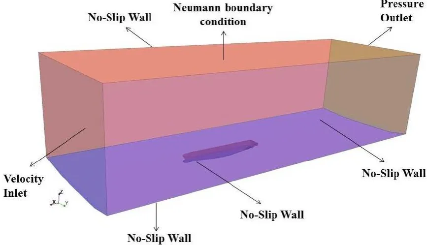
In all CFD problems, the initial conditions and boundary conditions must be defined depending on the physics of the problem to be solved. The determination of these boundary conditions is of critical importance in order to be able to obtain accurate solutions. There are a vast number of boundary condition combinations that can be used to approach a problem. However, the selection of the most appropriate boundary conditions can prevent unnecessary computational costs when approaching the problem [33]. A general view of the computational domain with the DTC hull model and the notations of selected boundary conditions are depicted in Figure 5.

Figure 5 delineates that a velocity inlet boundary condition was set in the positive x-direction, where flat waves were generated. The initial flow velocity at this inlet condition was set to the corresponding velocity of the flat waves. Conversely, the negative x-direction was modelled as a pressure outlet since it prevents backflow from occurring and fixes static pressure at the outlet. On the top of the domain, a Neumann boundary condition with static pressure equal to the reference pressure (0 Pascal) was applied to mimic the tank conditions. The bottom boundary was selected as a no-slip wall to account for the presence of the tank-floor. Similarly, the two sides of the domain (y-direction) have no-slip wall boundary conditions so that the tangential velocity is explicitly set to zero. Prabhakara and Deshpande [34] point out that, “a moving fluid in contact with a solid body will not have any velocity relative to the body at the contact surface. This condition of not slipping over a solid surface has to be satisfied by a moving fluid. This is known as the no-slip conditions”. Also, it is known that for no-slip walls in turbulent flow, only the component of velocity parallel to the wall is of interest [30].

Date and Turnock [33] emphasize that just as the selection of the boundaries is of great importance, their positioning is equally important. CD-Adapco [30] recommends that for trim, sinkage and resistance simulations, the inlet boundary should be located at least 1LBP away from the hull,

whereas the outlet should be positioned at least 2LBP downstream to avoid any wave reflection from

the boundary walls. Therefore, in this study, the inlet boundary was positioned 1.22LBP away from

the hull, and the outlet boundary 2.23LBP downstream. It is worth mentioning that throughout all the

software package was applied to the solution domain with a damping length equal to approximately 1.127LBP (10 m). This numerical beach model was used in upstream and downstream directions.

5.4 Coordinate Systems

Two different coordinate systems were adopted to predict the squat and resistance of the ship in calm water. Firstly, the flow field was solved, and the excitation forces and moments acting on the ship hull were calculated in the earth-fixed coordinate system. Following this, the forces and moments were converted to a body local coordinate system which was located at the centre of mass of the body, following the motions of the body whilst the simulation progressed. The equations of motions were solved to calculate the vessel’s velocities. These velocities were then converted back to the earth-fixed coordinate system. These sets of information were then used to find the new location of the computational domain [35].

5.5 Mesh Generation

Mesh generation was performed using the automatic meshing facility in STAR-CCM+, resulting in a computation mesh of circa 7 million cells in total. A trimmed cell mesher was employed to produce a high-quality grid for complex mesh generating problems. The ensuing mesh was formed primarily of unstructured hexahedral cells with trimmed cells adjacent to the surface. The mesh was rigid and body-fixed, so that motions of the body corresponded to the movement of grid points.

The computation mesh had areas of progressively refined mesh size in the area immediately around the hull, rudder and propeller, as well as the expected free surface and in the wake that was produced by the ship, to ensure that the complex flow features were appropriately captured. The refined mesh density in these zones was achieved using volumetric controls applied to these areas. The rate at which cell sizes increase from one cell size to another within the trimmed cell mesh was controlled by the ‘template growth rate’. In this study, in order to avoid abrupt mesh transitions between the refinements, a slow growth rate was applied, which allows the mesher to use multiple cell layers per transition to facilitate a gradual mesh transition.

Figure 6 depicts a cross-sectional view of the volume mesh generated inside the computational domain. Figure 7 provides a closer look at the volume mesh generated around the free surface. Since the computational domain is very large, for visual convenience the figure consists of two separate snapshot pictures. Figure 8 displays the surface mesh on the ship stern with propeller and rudder.

a ‘prism mesh model’ was employed to allow the RANS solver to create orthogonal prismatic cells next to wall boundaries, which ensures a higher degree of accuracy can be achieved for the flow solution. A fine mesh around the vessel was therefore automatically generated due to the application of a slow growth ratio during the meshing stage.

6. RESULTS AND DISCUSSION

The following section will outline the simulation results achieved during this study, and will also provide some comparison with experimental results. It will then present a discussion on the observation of the results. This section is divided into four main sub-sections, each of which presents different aspects of this work’s findings. Before proceeding to examine the results obtained, it is first necessary to perform a verification study.

6.1 Verification Study

A verification study was undertaken to estimate the discretization errors due to grid-size and time-step resolutions for Case 11 (which has a high Fnh in a moderate draft value). It is expected that the

numerical uncertainties for the other cases are of the same order.

Xing and Stern [36] state that the Richardson extrapolation (RE) method [37] is the basis for existing quantitative numerical error/uncertainty estimates for time-step convergence and grid-spacing. With this method, the error is expanded in a power series, with integer powers of grid-spacing or time-step taken as a finite sum. Commonly, only the first term of the series will be retained, assuming that the solutions lie in the asymptotic range. This practice generates a so-called grid-triplet study. Roache’s [38] grid convergence index (GCI) is useful for estimating uncertainties arising from grid-spacing and time-step errors. Roache’s GCI is recommended for use by both the American Society of Mechanical Engineers (ASME) [39] and the American Institute of Aeronautics and Astronautics (AIAA) [40].

For estimating iterative errors, the procedure derived by Roy and Blottner [41] was used. The results obtained from these calculations suggest that the iterative errors for squat and the total resistance coefficient (CT) are equal to almost zero.

Grid-spacing and time-step convergence studies were carried out following the GCI method described in Celik et al. [39]. The convergence studies were performed with triple solutions using systematically refined grid-spacing or time-steps. For example, the grid convergence study was conducted using three calculations in which the grid size was systematically coarsened in all directions whilst keeping all other input parameters (such as time-step) constant. The mesh convergence analysis was carried out with the smallest time-step, whereas the time-step convergence analysis was carried out with the finest grid size.

To assess the convergence condition, the convergence ratio (Rk) is used, as given by:

where εk21=φk2-φk1 and εk32=φk3-φk2 are the differences between medium-fine and coarse-medium

solutions, and φk1, φk2 and φk3 correspond to the solutions with fine, medium and coarse input

parameters, respectively. The subscript k refers to the kth _{input parameter (i.e. grid-size or time-step)}

[42].

Four typical convergence conditions may be seen: (i) monotonic convergence (0<Rk<1), (ii)

oscillatory convergence (Rk<0; |Rk|<1), (iii) monotonic divergence (Rk>1), and (iv) oscillatory

divergence (Rk<0; |Rk|>1). For diverging conditions (iii) and (iv), neither error nor uncertainty can

be assessed [42]. For convergence conditions, the generalized RE method is applied to predict the error and order-of-accuracy (pk) for the selected kth input parameter. For a constant refinement ratio

(rk), pk can be calculated by:

32 21

ln(

/

)

ln( )

p

r







₍₈₎

The extrapolated values can be calculated from [39]:

21

1 2

(

) / (

1)

r

r





 





(9)

The approximate relative error and extrapolated relative error can then be calculated using Equations 10 and 11, respectively [39]:

21 1 2

1

a

e

 







(10)

e











(11)

Finally, the fine-grid convergence index is predicted by:

21 21

1.25

1

e

GCI

r





(12)

It should be borne in mind that the Equations 8-12 are valid for a constant rk value. Reference can

be made to [39] for the formulae valid for a non-constant refinement ratio. The notation style of this reference was used in this study in order to enable the verification results to be presented clearly.

conducted with triple solutions using systematically lessened time-steps, starting from Δt=0.00707L/V.

The verification parameters of the squat and the total resistance coefficients for the grid spacing and time-step convergence studies are presented in Tables 5 and 6, respectively.

As can be seen from Tables 5 and 6, reasonably small levels of uncertainty were estimated for the obtained parameters. The numerical uncertainties in the finest-grid solution for squat and CT are

predicted as 0.09% and 3.00%, respectively (Table 5). These values change to 0.60% and 0.00%, respectively, when calculating the numerical uncertainty in the smallest time-step solution (Table 6). It can be interpreted that the very small uncertainty results for the time-step convergence study are due to the selection of very small time-step resolutions in the simulations. Also, it is obvious that the total resistance coefficient is more sensitive to the grid-spacing compared to the ship squat.

6.2 Wave Pattern

In this sub-section, wave contours generated by the presence of the ship model free to trim and sink around a free surface are presented. Figure 9 illustrates the wave patterns around the container ship model in question, for various depth Froude numbers (Fnh=0.475, 0.515 and 0.544), for a full-scale

draft of 14 m. As can be seen from the figure, as the depth Froude number increases, the length of the transverse waves increases. Another interesting result that can be drawn from the figure is that the wave contours become densely massed along the slope on each side of the canal. Since the canal is asymmetric and has different slope gradients on each side, the length and appearance of the waves generated on the port and starboard sides of the canal are different. In other words, asymmetric wave patterns are obtained by the existence of a ship advancing through an asymmetric canal in calm water.

The pictures given in Figure 9 clearly show the trajectories of the waves, firstly generated by the presence of the vessel and then reflected from the side walls of the canal. These reflected waves then dissipate as they propagate towards the mid-canal aft of the vessel.

The wave contours around the vessel are remarkably affected by the ship’s forward speed. This manifests itself as the Kelvin wake pattern, such that this Kelvin wave pattern is clearly visible in Case 12 (Figure 9c), where the vessel speed is the highest. It should also be mentioned that, for the reasons explained in Section 5.5, the area around the vessel was gradually refined in mesh size. Ideally, the whole free surface should have the same, fine, mesh size as the one around the vessel, though in this work a compromise was made between the mesh topology and the run time, in order to avoid an overly-long run time. The wave patterns around the vessel are therefore affected by this mesh transition between the refinements. This can be particularly seen from Figure 9a. Having said that, these authors believe that the change in mesh topology does not significantly affect the squat and resistance results. The mesh dependence study provided in Table 5 also supports this claim.

6.3 Squat Results

The dynamic sinkage results of the DTC model advancing through the canal non-dimensionalised with the ship length are presented for three ship drafts in Table 7. As mentioned earlier, the squat results obtained using the proposed RANS method were compared to those obtained from the experimental work of [5]. The table also covers the comparison errors based on experimental data.

The squat results, listed in Table 7, are illustrated graphically in Figure 10. This gives a clearer depiction of the ship squat against ship speed for different drafts, enabling a more facile comparison among the CFD and Experimental Fluid Dynamics (EFD) approaches.

As Table 7 and Figure 10 jointly show, the ship squat increases with increasing depth Froude number, or ship speed. In addition to this, for a constant speed, the vessel demonstrates more squat with a larger draft. Also, it is interesting to note that if the full-scale draft increases in magnitude by 1 m from T=13 m to T=14 m, the squat change only becomes more pronounced at Fnh values above

0.4 (which roughly corresponds to a full-scale speed of 10 knots). However, as the magnitude of the full-scale draft increases only slightly more to a value of T=14.5 m, then this has a major effect on the squat values across all of the depth Froude numbers involved.

The numerically predicted squat at the ship’s CoG agrees well with the model test measurements. Table 7 clearly states that the employed CFD model predicts ship squats within 10% of the experimental values. The CFD results tend to underestimate the magnitude of the expected squat, compared to the towing tank experiments. It should be noted that the standard deviations of the experimental squat results are reported to be within the range of 10% [5]. The discrepancies between the experimental and numerical results may therefore be attributed to high standard deviations of the squat measurement. As explicitly pointed out in [5], during the towing tank experiments conducted for the DTC model, more squat values are observed at the ship’s stern compared to those measured at the ship’s CoG.

6.4 Resistance Results

The total resistance (drag) of a ship is mainly composed of two components; the frictional resistance (RF) and pressure resistance (RP) as given by Equation 13. The latter component is made up of the

wave-making resistance (RW) and the viscous pressure resistance (RVP).

T F P

R



R



R

(13)

Equation 13 can also be expressed in its more common non-dimensional form. This is achieved by dividing each term by 0.5ρV2_{S. S is the mean wetted surface of the vessel, calculated to be}

12.931 m2_{, 13.619 m}2 _{and 13.970 m}2 _{(for a model-scale ship). These values correspond to full-scale}

drafts of 13 m, 14 m, and 14.5 m, respectively. The total resistance coefficient CT is therefore

composed of the frictional resistance coefficient CF and the pressure resistance coefficient CP.

The data contained in Table 8 are graphically shown in Figure 11, to enable a clearer comparison among the resistance coefficients obtained for three different loading conditions. As can be seen from both Table 8 and Figure 11, the resistance coefficients are highly affected by the ship’s draft, as expected. For all resistance components, the drag forces increase with larger ship draft. Also, at low speeds, the frictional resistance provides the largest contribution to the total resistance, whereas at higher speeds, the pressure resistance becomes dominant. More interestingly, the depth Froude number value at which the pressure resistance starts to become dominant varies with changing ship draft. Figure 11 illustrates that the critical Fnh values are circa 0.53, 0.42 and 0.22 for full-scale ship

drafts of 13 m, 14 m and 14.5 m, respectively. That means the critical Fnh value decrease as the ship

draft increases. This shift in the critical depth Froude number may be attributed to two factors:

i) As the ship draft increases, in other words, as the ship sits deeper in the water, its water plane area changes. This in turn affects the wave making resistance of the ship, owing to the hull form.

ii) As the ship draft increases, the ratio of the water depth to the ship draft (h/T) decreases, so the shallow water effects becomes more drastic. As pointed out in many papers (for example [4, 21, 43]), this ultimately leads to an increase in wave making resistance and hence in pressure resistance. Therefore, in the deepest ship draft condition, i.e. in the smallest h/T ratio, the increase in wave making resistance becomes the largest. Consequently, this makes the pressure resistance become dominant even at very low ship speeds (or Froude numbers).

In order to reveal the shallow water effect of a ship advancing through a canal on its resistance characteristics, and to eliminate the other factors influencing ship resistance, such as ship form, the same analyses should be repeated in deep water conditions. This is left as a piece of future research as this would require the creation of a further eighteen simulations to be run in deep water conditions.

7. CONCLUDING REMARKS

Fully nonlinear unsteady RANS simulations were performed to predict the squat and resistance of a model-scale DTC container ship for three different ship drafts at a range of forward speeds. The ship speeds and draft values were selected in analogy to the towing tank experiments of [5]. All analyses were performed using a commercial RANS solver, Star-CCM+, version 9.0.2.

Firstly, a verification study was performed for Case 11, following the procedure of [39]. The results showed that reasonably small levels of uncertainty were predicted for the squat and the total resistance coefficient. The numerical uncertainties in the finest-grid solution for sinkage and CT were

calculated to be 0.09% and 3.00%, respectively. These values altered to 0.60% and 0.00%, respectively, for the numerical uncertainty in the smallest time-step solution.

Following this, the dynamic sinkage results of the model scale DTC container ship obtained from the CFD simulations were presented at a range of ship forward speeds for three different ship drafts. The numerical squat results were also compared to those from available experiments. A comparison showed that the squat results obtained using CFD were only underpredicted within 10% of the EFD data. However, the standard deviations of the experimental squat results are given to be within the range of 10%.

It was concluded that ship squat increases with increasing ship speeds, as expected. Also, it was shown that the vessel demonstrates more squat with an increasing draft. Another interesting result drawn from the analyses was that a slight increase in magnitude to a larger draft may have more of an effect on ship squat than a much larger increase in magnitude applied to a smaller initial draft.

Finally, resistance results were presented for the model-scale DTC container ship. For all simulation cases, the two resistance components (frictional and pressure) that contributed to the total resistance were given in standard tabular and graphical formats. As clearly shown in the paper, the ship resistance was very sensitive to ship draft. A larger ship draft produces higher drag forces. Also, it was demonstrated that at low depth Froude numbers, the frictional resistance gave the largest contribution to the total resistance. In this paper, the depth Froude number where the pressure resistance begins to become dominant has been termed the critical depth Froude number. It was interesting to note that as a ship’s draft increases, this critical Fnh value of the ship in question

becomes diminished. The reasons for this were attributed to two factors, which discussed in detail in the paper.

This study has provided a different aspect for investigations into the resistance of a ship travelling through a canal, from a CFD point of view. The discussion made in the paper for the change in the critical depth Froude number for varying ship draft will be extended, by running the same simulations in deep water conditions. The study should also be extended to investigate the effect of other parameters, such as channel width, on squat and drag forces. In this study, trim values were not assessed as they are not of prominent importance in the sub-critical speed regime. Therefore, a piece of future work may be to incorporate trim behaviour of the vessel under all three speed regimes. Moreover, since the experiments were conducted in an asymmetric canal, the sway force and yawing moment of the ship are also of great importance. For this reason, by using the proposed RANS method, calculations to investigate the sway force and yawing moment should be performed for a vessel advancing through an asymmetric canal, as this would be another interesting piece of novel research.

ACKNOWLEDGEMENTS

The results were obtained using the EPSRC funded ARCHIE-WeSt High Performance Computer (www.archie-west.ac.uk). EPSRC grant no. EP/K000586/1.

REFERENCES

1. Tuck EO (1978) Hydrodynamic problems of ships in restricted waters. Annual Review of Fluid Mechanics 10:33-46, DOI: 10.1146/annurev.fl.10.010178.000341

2. Barrass B, Derret DR (2012) Ship Stability for Masters and Mates (7th edn). Elsevier, USA

3. Briggs MJ (2006) Ship squat predictions for ship/tow simulator, US army Corps of Engineers

4. Beck RF, Newman JN, Tuck EO (1975) Hydrodynamic forces on ships in dredged channels. Journal of Ship Research 19(3):166-171

5. Uliczka K (2010) Fahrdynamisches verhalten eines groben containerschiffs in seiten- und tiefenbegrenztem fahrwasser. Bundesanstalt für Wasserbau, Hamburg

6 Havelock TH (1908) The propagation of groups of waves in dispersive media, with application to waves on water produced by a travelling disturbance. Proceedings of the Royal Society of London Series a-Containing Papers of a Mathematical and Physical Character 81(549):398-430, DOI: 10.1098/rspa.1908.0097

7. International Navigation Association (2003) Guidelines for managing wave wash from high-speed vessels. PIANC, Brussels, Belgium

8. Varyani KS (2006) Squat effects on high speed craft in restricted waterways. Ocean Engineering 33(3-4):365-381, DOI: 10.1016/j.oceaneng.2005.04.016

9. Kreitner J (1934) Uber den Schiffswiderstand auf beschrankter Wasser. Werft Reederei Hafen

10. Constantine T (1960) On the movement of ships in restricted waterways. Journal of Fluid Mechanics 9(2) 247-256, DOI: 10.1017/s0022112060001080

11. Tuck EO (1966) Shallow-water flows past slender bodies. Journal of Fluid Mechanics 26(1):81-95, DOI: 10.1017/s0022112066001101

12. Tuck EO (1967) Sinkage and trim in shallow water of finite width. Schiffstechnik 14(73):92-94

13. Yasukawa HA (1993) Rankine panel method to calculate steady wave-making resistance of a ship taking the effect of sinkage and trim into account. Transactions of the West Japan Society of Naval Architects 86:27-35

14. Jiang T (1998) Investigation of waves generated by ships in shallow water. 22nd Symposium on Naval Hydrodynamics, Washington DC, USA: 601-612

15. Gourlay T (2008) Slender-body methods for predicting ship squat. Ocean Engineering 35(2):191-200, DOI: 10.1016/j.oceaneng.2007.09-001

16. Gourlay T (2008) Sinkage and trim of a fast displacement catamaran in shallow water. Journal of Ship Research 52(3):175-183

17. Alderf N, Lefrançois E, Sergent P, Debaillon P (2011) Dynamic ship response integration for numerical prediction of squat in highly restricted waterways. International Journal for Numerical Methods in Fluids 65(7):743-763, DOI: 10.1002/fld.2194

18. Yao JX, Zou ZJ (2010) Calculation of ship squat in restricted waterways by using a 3D panel method. Journal of Hydrodynamics 22(5):472-477, DOI:

10.1016/S1001-6058(09)60241-9

19. Alidadi M, Calisal S (2011) A numerical study on squat of a Wigley hull. ASME 30th International Conference on Ocean, Offshore and Arctic Engineering, Vol 7: CFD and Viv: Offshore Geotechnics: 539-543, Rotterdam, The Netherlands

20. Jachowski J (2008) Assessment of ship squat in shallow water using CFD. Archives of Civil and Mechanical Engineering 8(1):27-36

21. Prakash S, Chandra B (2013) Numerical estimation of shallow water resistance of a river-sea ship using CFD. International Journal of Computer Applications 71(5):33-40 22. Wortley S (2013) CFD analysis of container ship sinkage, trim and resistance. Curtin University, Department of Mechanical Engineering, B.Eng Mechanical Engineering Project Report No. 491/493, Bentley, Western Australia

23. He W, Castiglione T, Kandasamy M, Stern, F (2014) Numerical analysis of the interference effects on resistance, sinkage and trim of a fast catamaran . Journal of Marine Science and Technology:1-17, DOI: 10.1007/s00773-014-0283-0

25. Mucha P, El Moctar O, Bottner CU (2014) Technical note : PreSquat - Workshop on numerical prediction of ship Squat in restricted waters. Ship Technology Research: Schiffstechnik 61(3):162-165

26. PreSquat (n.d.) Instructions- Dynamic squat test parameter. Accessed: 01/11/2014, https://www.uni-due.de/IST/ismt_presquat_test.shtml

27. Ferziger JH, Peric M (2002) Computational Methods for Fluid Dynamics (3rd edn). Springer, Berlin

28. Tezdogan T, Demirel YK, Kellett P, Khorasanchi M, Incecik A, Turan O (2015) Full-scale unsteady RANS CFD simulations of ship behaviour and performance in head Seas due to slow steaming. Ocean Engineering 97:186-206, DOI: 10.1016/j.oceaneng.2015.01.011 29. Tezdogan T, Incecik A, Turan O (2015) Full-scale unsteady Reynolds-Averaged Navier-Stokes simulations of vertical ship motions in shallow water. Submitted to Applied Ocean Research (under review)

30. CD-Adapco (2014) User guide STAR-CCM+ (Version 9.0.2).

31. Querard A, Temarel P, Turnock SR (2008) Influence of viscous effects on the hydrodynamics of ship-like sections undergoing symmetric and anti-symmetric motions, using RANS. Proceedings of the 27th International Conference on Offshore Mechanics and Arctic Engineering 5:683-692

32. International Towing Tank Conference (ITTC) (2011) Practical guidelines for ship CFD applications. 26th ITTC

33. Date JC, Turnock SR (1999) A study into the techniques needed to accurately predict skin friction using RANS solvers with validation against Froude’s historical flat plate

experimental data. University of Southampton, Southampton, England, Ship Science Reports 114

34. Prabhakara S, Deshpande MD (2004) The no-slip boundary condition in fluid mechanics. Resonance 9(4):50-60, DOI: 10.1007/BF02834856

35. Simonsen CD, Otzen JF, Joncquez S, Stern F (2013) EFD and CFD for KCS heaving and pitching in regular head waves. Journal of Marine Science and Technology 18(4):435-459, DOI: 10.1007/s00773-013-0219-0

36. Xing T, Stern F (2010) Factors of Safety for Richardson Extrapolation. Journal of Fluids Engineering-Transactions of the ASME 132(6):061403, DOI: 10.1115/1.4001771 37. Richardson LF (1911) The approximate arithmetical solution by finite differences of physical problems involving differential equations, with an application to the stresses in a Masonry dam. Philosophical Transactions of the Royal Society of London Series A-Containing Papers of a Mathematical or Physical Character 210:307-357, DOI: 10.1098/rsta.1911.0009 38. Roache PJ (1998) Verification and Validation in Computational Science and

Engineering. Hermosa Publishers, Albuquerque

39. Celik IB, Ghia U, Roache PJ, Freitas CJ (2008) Procedure for estimation and reporting of uncertainty due to discretization in CFD applications. Journal of Fluids Engineering-Transactions of the ASME 130(7):078001, DOI: 10.1115/1.2960953

40. Cosner RR, Oberkampf WL, Rumsey CL, Rahaim CP, Shih TIP (2006) AIAA Committee on standards for computational fluid dynamics: Status and plans. 44th Aerospace Sciences Meeting and Exhibit, Reno, Nevada

41. Roy CJ, Blottner FG (2001) Assessment of one- and two-equation turbulence models for hypersonic transitional flows. Journal of Spacecraft and Rockets 38(5):699-710

42. Stern F, Wilson R, Shao J (2006) Quantitative V&V of CFD simulations and certification of CFD codes. International Journal for Numerical Methods in Fluids 50(11): 1335-1355, DOI: 10.1002/fld.1090

Fig. 1 Ship in a canal in its static condition, taken from [2].

Fig. 2 Hull sections of DTC container ship, taken from [24].

Fig. 3 A three-dimensional view of the DTC container ship, modelled in Star-CCM+.

Fig. 4 Cross-section of the asymmetric canal through which the vessel is advancing, adapted from [26].

Fig. 5 A general view of the computational domain and the applied boundary conditions.

Fig. 6 Cross-sectional view of the volume mesh inside the computational domain.

Fig. 7 A cross-sectional view of the volume mesh from above, around the entire free surface: a) the upper half shows downstream, and b) the lower half shows

Fig. 8 Surface mesh on the ship stern with rudder and propeller.

Fig. 9 Comparison of wave patterns generated around the model-scale ship, for various depth Froude numbers (a) Fnh=0.475 (Case 10), (b) Fnh=0.515 (Case 11), (c) Fnh=0.544 (Case 12).

Fig. 10 Comparison of the non-dimensionalised squat values obtained at ship’s CoG, using EFD and CFD methods in three different ship drafts against various depth Froude numbers.

(a)

(b)

(c)

Figure 9. Comparison of wave patterns generated around the model-scale ship, for various depth Froude numbers (a) Fnh=0.475 (Case 10), (b) Fnh=0.515 (Case 11), (c)

Figure 10. Comparison of the non-dimensionalised squat values obtained at ship’s CoG,

Figure 11. Graph of the total resistance coefficient CT of the model-scale DTC against a

range of depth Froude numbers for (a) full-scale draft T=13 m, (b) T=14 m, (c) T=14.5 m. The dashed lines and centre lines show the contributions of the resistance

Table 1 Full scale and model scale DTC properties [24].

Table 2 Cross-section dimensions of the canal in full scale, taken from [26].

Table 3 The cases to which the CFD model is applied.

Table 4 The final cell numbers for each mesh configuration as a result of the mesh convergence study.

Table 5 Grid convergence study for sinkage and total resistance coefficient.

Table 6 Time-step convergence study for sinkage and total resistance coefficient.

Table 7 The squat results for all cases by the current CFD and EFD (Error is based on EFD data).

Table 1. Full scale and model scale DTC properties [24].

Property Ship Model (1:40)

Length between the perpendiculars (LBP) 355 m 8.875 m

Beam at waterline (BWL) 51 m 1.275 m

Design draft (T) 14.5 m 0.3525 m

Displacement (Δ) 173,814.762 m3 _{2.716 m}3

Block coefficient (CB) 0.661 0.661

Ship wetted area with rudder and propeller (S) 22352 m2 _{13.970 m}2

Longitudinal centre of buoyancy (LCB) from the aft peak 174.531 m 4.363 m

Vertical centre of gravity (KG) from keel 23.28 m 0.582 m

Metacentric height (GMt) 1.677 m 0.042 m

Moment of inertia (Kxx/B) 0.40 0.40

Table 2. Cross-section dimensions of the canal in full scale, taken from [26].

Parameters Value (m)

H 16

L1 160

L2 128

L3 166

Table 3. The cases to which the CFD model is applied. Case No Full-Scale Draft (m) Ship Speed Depth Froude Number Full Scale (kn) Model Scale (m/s) 1 13.0

5.07 0.412 0.208

2 7.35 0.598 0.302

3 10.60 0.862 0.435

4 11.99 0.975 0.492

5 12.92 1.051 0.530

6 13.59 1.105 0.558

7

14.0

4.80 0.390 0.197

8 6.81 0.554 0.280

9 8.34 0.678 0.342

10 11.57 0.941 0.475

11 12.54 1.020 0.515

12 13.25 1.078 0.544

13

14.5

2.42 0.197 0.099

14 6.35 0.516 0.261

15 7.98 0.649 0.328

16 9.71 0.790 0.399

17 11.16 0.908 0.458

Table 4. The final cell numbers for each mesh configuration as a result of the mesh convergence study.

Mesh

Configuration Total cell number

Fine 6,963,044

Medium 4,378,144

Table 5. Grid convergence study for sinkage and total resistance coefficient.

Squat at CoG/LBP

(with monotonic convergence)

CT

(with monotonic convergence)

r √2 √2

φ1 -0.00279 0.008258

φ2 -0.00280 0.008085

φ3 -0.00281 0.007761

R 0.308 0.534

p 3.40 1.81

φext21 0.002789 0.0084562

ea21 0.16% 2.09%

eext21 0.07% 2.34%

Table 6. Time-step convergence study for sinkage and total resistance coefficient.

Squat at CoG/LBP

(with monotonic convergence)

CT

(with monotonic convergence)

r √2 √2

φ1 -0.00279 0.008258

φ2 -0.00277 0.008257

φ3 -0.00272 0.008036

R 0.4 0.005

p 2.64 15.58

φext21 0.0028033 0.008258

ea21 0.72% 0.01%

eext21 0.48% 0.00%

Table 7. The squat results for all cases by the current CFD and EFD (Error is based on EFD data).

Case No Full Scale _{Draft (m)} Froude Depth Number

CFD EFD

Error (%) Squat at

CoG/LBP

Squat at CoG/LBP

1

13.0

0.208 -0.000201 -0.000183 9.57

2 0.302 -0.000684 -0.000732 -6.65

3 0.435 -0.001624 -0.001662 -2.30

4 0.492 -0.002193 -0.002338 -6.22

5 0.530 -0.002771 -0.003000 -7.62

6 0.558 -0.003477 -0.003789 -8.22

7

14.0

0.197 -0.000200 -0.000183 9.16

8 0.280 -0.000593 -0.000620 -4.39

9 0.342 -0.001000 -0.001014 -1.35

10 0.475 -0.002175 -0.002296 -5.27

11 0.515 -0.002791 -0.002873 -2.85

12 0.544 -0.003339 -0.003634 -8.13

13

14.5

0.099 -0.000015 -0.000014 7.90

14 0.261 -0.000612 -0.000648 -5.57

15 0.328 -0.000984 -0.001085 -9.26

16 0.399 -0.001586 -0.001577 0.55

17 0.458 -0.002276 -0.002282 -0.26

Table 8. The resistance coefficients for the DTC in model scale, obtained using the current CFD model.

Case No Full Scale _{Draft (m)} Depth Froude _{Number Number} Froude

Resistance Coefficientsx10-3

Pressure (CP)

Frictional

(CF) Total (CT)

1

13

0.208 0.044 3.714 4.087 7.801

2 0.302 0.064 2.779 3.732 6.511

3 0.435 0.092 3.059 3.618 6.677

4 0.492 0.105 3.170 3.607 6.777

5 0.530 0.113 3.661 3.629 7.290

6 0.558 0.118 4.125 3.688 7.813

7

14

0.197 0.042 4.048 4.049 8.097

8 0.280 0.059 3.357 3.732 7.089

9 0.342 0.073 3.262 3.689 6.952

10 0.475 0.101 4.013 3.634 7.646

11 0.515 0.109 4.568 3.691 8.258

12 0.544 0.115 5.072 3.736 8.808

13

14.5

0.099 0.021 4.567 5.342 9.909

14 0.261 0.055 3.988 3.872 7.860

15 0.328 0.070 4.283 3.775 8.058

16 0.399 0.085 3.934 3.724 7.658

17 0.458 0.097 5.145 3.669 8.814