Improving the boundary efficiency of a compact finite
difference scheme through optimising its composite
template
Jacob M. Turner∗, Sina Haeri∗∗, Jae Wook Kim
Aerodynamics and Flight Mechanics Research Group, University of Southampton, Southampton, SO17 1BJ, UK
Abstract
This paper presents efforts to improve the boundary efficiency and accu-racy of a compact finite difference scheme, based on its composite template. Unlike precursory attempts the current methodology is unique in its quan-tification of dispersion and dissipation errors, which are only evaluated after the matrix system of equations has been rearranged for the derivative. This results in a more accurate prediction of the boundary performance, since the analysis is directly based on how the derivative is represented in simulations. A genetic algorithm acts as a comprehensive method for the optimisation of the boundary coefficients, incorporating an eigenvalue constraint for the linear stability of the matrix system of equations. The performance of the optimised composite template is tested on one-dimensional linear wave con-vection and two-dimensional inviscid vortex concon-vection with uniform and curvilinear grids. In all cases, it yields substantial accuracy and efficiency
∗
Corresponding author,Email address: [email protected]
∗∗
improvements while maintaining stable solutions and fourth-order accuracy.
Keywords: Compact finite difference; Boundary closure; Optimization; Genetic algorithm; Composite template
1. Introduction
1
Compact finite differences are numerical schemes used to accurately cal-2
culate derivatives. They are implicit in nature, based upon a banded Hermi-3
tian matrix system of equations. Although inverting such a system requires 4
a higher computational cost, they can offer vastly superior resolution for a 5
given stencil size compared to their explicit counterparts. This quality has 6
made them increasingly popular in the fields of computational aeroacoustics 7
(CAA) [1, 2], large eddy simulation (LES) [3–5], and direct numerical simu-8
lation (DNS) [6–8], particularly when high resolution is a necessity in order 9
to properly resolve the relevant physical scales. 10
Typically, central differences are used to construct compact schemes for 11
use at interior nodes. However, such schemes are not always applicable at do-12
main boundaries, and therefore in order to properly close the matrix system 13
of equations non-central differences are often a necessity. This unfortunately 14
will have a detrimental effect on accuracy; introducing additional dissipa-15
tion as well as dispersion, if the boundary schemes are not sufficiently opti-16
mised. Consequently, to ensure that the same level of accuracy is achieved 17
throughout the entire domain, grid refinements are regularly made to the 18
boundary regions. This will inevitably reduce computational efficiency due 19
to the decreased time step required by the smaller grid cells. The objective 20
performance, and thereby minimise efficiency losses, while also ensuring the 1
combination of interior and boundary schemes meets requirements for linear 2
stability. 3
As well as changes in formal order of accuracy, enhancements to compact 4
schemes can also be achieved through coefficient optimisation based on res-5
olution characteristics. A previous attempt at this was undertaken by Kim 6
[1]. Kim introduced a highly optimised fourth-order pentadiagonal compact 7
scheme and set of boundary closures particularly for CAA applications. Op-8
timisations were based on an integral error measure between the exact and 9
modified wavenumber solutions (similar to Kim and Lee [9]). Very low res-10
olution errors were obtained with this method, in particular for the interior 11
scheme, which remains below 0.1% over the grid spaced scaled wavenumber 12
range 0 ≤ ω ≤ 0.839π. The boundary schemes were designed to maintain 13
the same stencil size and order of accuracy as the interior schemes, which 14
was accomplished by employing extrapolation functions based on both poly-15
nomial and trigonometric series for solutions outside of the domain. After 16
some algebraic manipulation, these were then converted into a set of non-17
central differences for use at the domain boundaries. The resultant boundary 18
schemes were optimised by means of control variables left open in the trigono-19
metric series of each extrapolation function. As in Carpenter et al. [10] the 20
linear stability of the matrix system was investigated using eigenvalue anal-21
ysis. Kim [1] found that with a coarse grid the schemes contained some 22
slightly positive eigenvalue components. Although, after some grid refine-23
ment it was demonstrated that these will tend towards zero, hence implying 24
Liu et al. [11] expanded on the optimisation strategy of Kim [1] by intro-1
ducing a sequential quadratic programming technique (SQP). This iteratively 2
increased the upper limit of the optimisation range (r), establishing optimal 3
values for both interior and boundary schemes. Furthermore, they showed 4
that scheme stability is heavily dependent on the chosen error tolerances, as 5
well as the formal order of accuracy, implying that the optimisation process 6
can often be detrimental to the numerical stability. To compensate for this, 7
Liu et al. [11] reduced the order of accuracy of their first and third boundary 8
schemes by one stage. Such stability issues were also recognised by Carpenter 9
et al. [10], who suggested that a scheme’s numerical stability and its spectral 10
resolution do not always coincide. 11
Jordan [12] introduced an alternative approach for analysing spectral res-12
olution properties through composite templates. Unlike the more traditional 13
decoupled Fourier approach where the resolution of each differencing stencil 14
is studied separately, this consists of Fourier analysis of the whole matrix 15
system of equations, consisting of both the interior and boundary stencils. 16
The result is a set of pseudo-wavenumber curves for each point in the grid, 17
dependent on the number of grid points used in the analysis. Jordan applied 18
this analysis to tridiagonal systems, employing a least squares optimisation 19
strategy to minimise the total resolution error across the whole template. In 20
a later paper by Jordan [13] the same technique was applied to pentadiagonal 21
systems producing a set a of boundary closure schemes to be used alongside 22
the interior scheme of Kim [1]. Although the modified wavenumber curves 23
produced by this technique are dependent on the number of grid points used 24
mance we achieve once schemes are applied to actual simulations. Despite 1
this, it is still unclear how to best optimise the resolution properties of a 2
given composite template, making it far from a trivial task. For instance one 3
could prioritise minimising the relative resolution error between neighbouring 4
points in the composite template, or perhaps the aggregate resolution error 5
of the whole template with respect to the exact wavenumber. 6
This paper aims to extend the composite template strategy of Jordan 7
[12] by redefining how the composite template modified wavenumber is eval-8
uated. Unlike the original approach, Fourier analysis will not be conducted 9
until the matrix system of equations has already been rearranged for the 10
derivative. This should lead to better predictions of the resolution prop-11
erties attained in simulations because this is a closer depiction of how the 12
derivative is represented numerically. The chosen optimisation method is a 13
Genetic Algorithm (GA) containing both an objective function for the com-14
posite template’s resolution characteristics, and a non-linear constraint for 15
eigenvalue stability. In this paper, the optimisation procedure is applied to 16
the pentadiagonal finite-difference system outlined by Kim [1], although a 17
similar approach would be applicable to other systems if desired. The newly 18
optimised boundary closure coefficients are successful in producing large ac-19
curacy improvements while maintaining stable solutions in all test problems. 20
In addition to the primary optimisation which focuses on the aggregate res-21
olution error of the composite template, further accuracy enhancements are 22
attempted by introducing pseudo-boundary schemes. Essentially these are 23
tuned central schemes applied as intermediate steps between the boundary 24
tween consecutive points. They are successful in achieving further accuracy 1
improvements, albeit with some penalty to numerical stability. 2
The paper is organised as follows. Section 2 introduces the compact 3
finite-difference system, and outlines the new composite template modified 4
wavenumber analysis. Section 3 provides details of the boundary closure 5
scheme coefficient optimisation procedure. Including the optimisation plat-6
form, objective function and stability constraints. Section 4 presents the 7
optimisation results, including the resultant wavenumber characteristics and 8
eigenvalue distribution. In section 5 the performance of the newly optimised 9
finite-difference system is tested in three benchmark problems, designed to 10
analyse their performance in a variety of scenarios. In section 6 pseudo-11
boundary schemes are introduced and their performance analysed. Finally 12
concluding remarks are given in section 7. 13
2. Compact Finite Difference Schemes and Composite Template
14
Modified Wavenumber Analysis
15
We consider the following general compact finite difference template, 16
based on a pentadiagonal Hermitian matrix. It is constructed from one cen-17
tral interior and three non-central boundary closure schemes, each in conser-18
vative form and utilising a seven-point stencil [1]. 19
P¯f′ = 1
hQf (1)
P =
1 γ01 γ02 0 · · · 0 0 0 0
γ10 1 γ12 γ13 0 · · · 0 0 0
γ20 γ21 1 γ23 γ24 0 · · · 0 0
0 β α 1 α β 0 · · · 0 ..
. . .. ... ... ... ... ... ... ... 0 · · · 0 β α 1 α β 0 0 0 · · · 0 γ24 γ23 1 γ21 γ20
0 0 0 · · · 0 γ13 γ12 1 γ10
0 0 0 0 · · · 0 γ02 γ01 1 Q=
b00 b01 b02 b03 b04 b05 b06 0 0 · · · 0
b10 b11 b12 b13 b14 b15 b16 0 0 · · · 0
b20 b21 b22 b23 b24 b25 b26 0 0 · · · 0 −a3 −a2 −a1 0 a1 a2 a3 0 0 · · · 0
0 −a3 −a2 −a1 0 a1 a2 a3 0 · · · 0
..
. . .. ... ... ... ... ... ... ... ... ... 0 · · · 0 −a3 −a2 −a1 0 a1 a2 a3 0
0 · · · 0 0 −a3 −a2 −a1 0 a1 a2 a3
0 · · · 0 0 −b26 −b25 −b24 −b23 −b22 −b21 −b20
0 · · · 0 0 −b16 −b15 −b14 −b13 −b12 −b11 −b10
0 · · · 0 0 −b06 −b05 −b04 −b03 −b02 −b01 −b00 and 1 ¯ f′ = ( ¯f′
0,f¯1′,f¯2′,· · · ,f¯N′ )T, f = (f0, f1, f2,· · · , fN)T
where ¯f′
i is a finite difference approximation to the exact spatial derivative 2
f′
i at a nodal point i and bii = − P6
j=0,6=ibij. The three boundary closure 3
schemes are applied at the i = {0, N}, {1, N −1} and {2, N −2} nodes. 4
They comprise of 27 unique coefficients: 5
γij for i={0,1,2} j ={0,· · · , i+ 2},6=i
bij for i={0,1,2} j ={0,· · · ,6},6=i.
The central interior scheme consists of five coefficients (α, β, a1, a2, a3), and
1
is applied throughout the remainder of the domain (3 ≤ i ≤ N −3). The 2
template we will consider in the current paper is fourth-order accurate in 3
the interior and at the boundaries. For the interior nodes we implement the 4
optimised fourth-order coefficients suggested by Kim [1]. (Full details of the 5
interior scheme performance, including its modified wavenumber character-6
istics can be found in [1].) 7
Fourier series decomposes a dependent function f into a number of os-8
cillatory functions also known as Fourier coefficients ˆf(k). For a domain of 9
N + 1 points (0,· · · , N) the discrete Fourier series can be expressed as 10
f(x) = N/2 X
k=−N/2
ˆ
f(k) exp
2πkx L
(3)
where =√−1,Lis the domain length, x is spatial coordinate, andk is the 11
wavenumber. This may be simplified by substituting for a scaled coordinate 12
x∗ =x/hand a scaled wavenumber ω= 2πkh/L, wherehis the grid spacing: 13
f(x) = N/2 X
k=−N/2
ˆ
f(k) exp (ωx∗). (4)
After realising that fi±m ≡f(x∗±m)), wherem ∈Z, it is possible to derive 14
an expression for a scaled modified wavenumber ¯ω by applying the Fourier 15
transform to each term in a differencing scheme. This differs from the exact 16
wavenumber ω due to numerical approximation, specifically f′ =ωf, while 17
¯
f′ =¯ωf (using Eq.(4)). 18
quantified using Fourier analysis, applied to each differencing stencil on an 1
individual basis (this procedure is described in detail in [14]). However, this 2
fails to take into account the fact that during actual simulations schemes are 3
not evaluated separately. Rather, they are implemented in a matrix system of 4
equations, as in Eq.(1). By inverting the matrix P, the following expression 5
for the spatial derivative at each nodal point can be obtained: 6
¯
f′ = 1
hTf (5)
where T = P−1Q. Consequently it seems appropriate to define a modified
7
wavenumber based on the spectral resolution of the whole composite tem-8
plate, by analysing each finite difference stencil in a coupled fashion. This 9
was first suggested by Jordan [12] whose composite template approach con-10
sists of taking the Fourier transform of each row of the matrix system in 11
Eq.(1). This results in a pseudo-wavenumber curve for each grid point, with 12
properties dependent on each other point used in the analysis. In the cur-13
rent paper we expand upon this approach by alternatively considering the 14
inverted matrix system given by Eq.(5). Applying the Fourier transform 15
sequentially to each row of this system result in the following: 16
jω¯f(k) exp(jωxˆ ∗)
jω¯f(k) exp(jω(xˆ ∗+ 1))
jω¯f(k) exp(jω(xˆ ∗+ 2))
...
jω¯fˆ(k) exp(jω(x∗+N))
=T ˆ
f(k) exp(jωx∗)
ˆ
f(k) exp(jω(x∗+ 1))
ˆ
f(k) exp(jω(x∗+ 2))
... ˆ
f(k) exp(jω(x∗+N))
After some algebraic manipulation this leads to an expression for the 1
coupled modified wavenumber of the composite template: 2
jω¯ =
T00+T01exp(jω) +T02exp(2jω) +· · ·+T0Nexp(Njκ) T10exp(−jω) +T11+T12exp(jω) +· · ·+T1N exp((N −1)jω)
...
TN0exp(−Njω) +TN1exp(−(N −1)jω)
+TN2exp(−(N −2)jω) +· · ·+TN N
(7) Here ¯ωis a vector of lengthN+1, representing the scaled modified wavenum-3
ber at each nodal point (0· · ·N). Each nodal element of ¯ω may also be 4
expressed in a more compact summation form as: 5
¯ ωi =−j
N X
m=0
Timexp(jω(m−i)) where i= 0,1,2,· · · , N (8)
where iand mrepresent the rows and columns of the matrix T. The disper-6
sion and dissipation errors approximated by Eq.(8) should provide a truer 7
depiction of the performance of the finite difference schemes, since the mod-8
ified wavenumber characteristics are now directly linked to the numerical 9
representation of the derivative. 10
3. Boundary Scheme Optimisation Framework
11
The chosen optimisation technique for the boundary scheme coefficients is 12
a genetic algorithm (GA) from the Matlab optimisation toolbox. This tech-13
to efficiently and robustly explore nonconvex objective functions and con-1
straints. The Matlab implementation of the GA conveniently handles the se-2
lection, crossover and mutation procedures of the optimisation. Additionally 3
it enables simple implementation of nonlinear inequality constraints which 4
prove useful for ensuring numerical stability of the resulting coefficients. For 5
an in-depth discussion of evolutionary optimisation techniques see [15]. 6
3.1. Formulation of Genetic Algorithm Independent Variables
7
The boundary closure schemes are constructed such that they preserve 8
both the truncation error and stencil size of the main interior scheme. Kim [1] 9
achieved this by introducing extrapolation functions based on both trigono-10
metric and fourth-order polynomial series to estimate function values beyond 11
the domain boundaries. By employing a series of constraints for the extrap-12
olation functions to match interior field values and derivatives, the originally 13
central schemes could then be rewritten as a set of non-central differences. 14
The new boundary closure coefficients could then be tuned by use of free 15
control variables left open in the trigonometric series. Similarly, in the cur-16
rent procedure the control variables are selected as the independent variables 17
for the GA, opposed to directly optimising each of the 27 unique boundary 18
closure coefficients. This approach reduces the number of GA independent 19
variables, reducing the complexity of the search task. Furthermore, it ensures 20
the resulting coefficients will obtain the desired fourth-order accuracy. This 21
is specified by the accuracy of the central scheme applied to the boundary 22
nodes and the order of the extrapolation function polynomial series. Origi-23
nally, Kim [1] proposed an individual extrapolation function for each bound-24
Alternatively, we choose to further simplify the procedure by applying the 1
i= 0 function to each boundary point (i= 0,1,2) resulting in just 3 control 2
variables. The three control variables used for optimisation in the GA are 3
herein referred to as φ1, φ2 and φ3. Each boundary closure coefficient can
4
be constructed as a non-linear function of these variables. Full details of the 5
extrapolation function and the constraints required to convert φ1−3 into the
6
boundary scheme coefficients can be found in [1]. 7
3.2. Genetic Algorithm Objective Function
8
The purpose of the objective function is to quantify the resolution prop-9
erties of the composite template so that it may be optimised. Ideally we 10
would like a composite template which produces no dispersion or dissipation 11
errors such that its modified wavenumber curves perfectly match the exact 12
wavenumber: 13
Re(¯ω)→ω (9)
Im(¯ω)→0. (10)
Here ¯ω is determined by Eq.(8) and ω is the exact scaled wavenumber. We 14
can represent this requirement as an integral error measure EA
i which we 15
require to tend to zero: 16
EA i |r0 =
Z r
0
[Re(¯ωi−ω) + Im(¯ω)]2dω 1
2
fori={0,1,2} (11)
An appropriate value for the integration range (r) is obtained by util-17
trial and error is then conducted to determine which r value produces the 1
most successful optimisation output. This is judged by the performance the 2
newly optimised schemes attain in the one-dimensional scalar wave bench-3
mark problem (section 5.1). This process resulted in a value of r = 0.52π. 4
Ideally we would like the modified wavenumber to match the exact wavenum-5
ber over the full range of scales from 0−π, and would therefore select r to 6
reflect this. However, this tends to result in very large overshoots at higher 7
wavenumbers. Additionally due to the dependence between each schemes 8
coupled modified wavenumber curves, a high integration range often results 9
in the improvement of one schemes resolution characteristics at the expense 10
of another. One possible solution would be to remove high frequencies with 11
filtering operations, however the low cut-off frequency required would greatly 12
degrade the solution obtained. Alternatively, by selecting a more moderate 13
r, the characteristics of each scheme tend to remain comparable over at least 14
a intermediate wavenumber range, resulting in far superior aggregate resolu-15
tion characteristics. The consequence of ignoring the higher wavenumbers in 16
the optimisation is a lack of control over wavenumber characteristics at high 17
frequencies. Despite this, the i = 1 and i = 2 schemes remained relatively 18
well behaved. The i = 0 scheme on the other hand was found to exhibit 19
a fairly large overshoot relative to the exact wavenumber between roughly 20
0.8π ≤ ω ≤ π, albeit reduced compared to an r = π case. To compensate
21
for this, an additional error measure EB is included, which aims to damp the 22
i= 0 overshoots over the appropriate range. 23
EB|π
0.8π =
Z π
0.8π
[Re(¯ω0−ω) + Im(¯ω)]2dω 1
2
CombiningEAand EB results in a final blended error measureE used as 1
the objective function in the GA 2
E =η
2 X
i=0
EA i |00.52π
!
+ (1−η)EB|π
0.8π (13)
where η is the weighting factor between the two error measures. If η is too 3
large, the overshoots at i = 0 are not sufficiently damped, however if η is 4
too small the aggregate resolution characteristics of the composite template 5
begin to suffer. A suitable value for η was selected through an equivalent 6
trial and error procedure as outlined for the integration range r, eventually 7
yielding a value of η= 0.948. 8
3.3. Linear Stability Constraint
9
In addition to exhibiting good resolution properties, and maintaining a 10
desired order of accuracy, a successful numerical scheme must also consis-11
tently provide stable solutions. In past procedures the numerical stability is 12
often treated as an afterthought, and is only considered after the wavenum-13
ber optimisation of the finite difference coefficients is completed ([1, 11–13]). 14
This usually results in the use of trial and error routines to obtain a re-15
sult which both achieves good performance and meets the desired stability 16
criteria. In the current work a more consistent optimisation strategy is es-17
tablished by integrating a non-linear constraint for eigenvalue stability into 18
the GA, ensuring the optimisation output is always satisfactory. 19
As pointed out by Liu et al. [11] and Carpenter et al. [10], the optimisation 20
process can often be detrimental to numerical stability, limiting the number 21
difference schemes are used in conjunction with a stabilising technique. In 1
this case we use the 6th order compact filters provided by Kim [16]. Compact 2
filters improve numerical stability by introducing a cut-off frequency. This 3
effectively removes unresolved wavenumber components from the solution at 4
the end of each time step. They are including via the following modifications 5
to Eq.(1): 6
P¯f′ = 1
hQ(f + ˜∆f) (14)
and 7
˜
∆f = ( ˜∆f0,∆f˜ 1,∆f˜ 2,· · · ,∆fN˜ )T, (15)
where ˜∆fi = ˜fi−fi represents the difference between filtered and unfiltered 8
values. A solution for ˜∆f can be obtained by solving the following matrix 9
system of equations 10
R∆˜f =Sf (16)
where
R=
1 γF
01 γ
F
02 0 · · · 0 0 0 0
γF
10 1 γ12F γ13F 0 · · · 0 0 0
γF
20 γF21 1 γ23F γ24F 0 · · · 0 0
0 βF αF 1 αF βF 0 · · · 0
..
. . .. ... ... ... ... ... ... ... 0 · · · 0 βF αF 1 αF βF 0
0 0 · · · 0 γF
24 γ23F 1 γ21F γ20F
0 0 0 · · · 0 γF
13 γF12 1 γ10F
0 0 0 0 · · · 0 γF
S=
0 0 0 0 0 0 0 0 0 · · · 0 0 0 0 0 0 0 0 0 0 · · · 0
bF
20 bF21 bF22 bF23 bF24 bF25 0 0 0 · · · 0
aF
3 aF2 aF1 aF0 aF1 aF2 aF3 0 0 · · · 0
0 aF
3 aF2 aF1 aF0 aF1 aF2 aF3 0 · · · 0
..
. . .. ... ... ... ... ... ... ... ... ... 0 · · · 0 aF
3 aF2 aF1 aF0 aF1 aF2 aF3 0
0 · · · 0 0 aF
3 aF2 aF1 a0F aF1 aF2 aF3
0 · · · 0 0 0 bF
25 bF24 bF23 bF22 bF21 bF20
0 · · · 0 0 0 0 0 0 0 0 0 0 · · · 0 0 0 0 0 0 0 0 0
superscript F denotes a filter coefficient, aF
0 = −2(aF1 + aF2 +aF3), and
1
bF
22=−(bF20+bF21+bF23+bF24+bF25).
2
The filter coefficients for each point are calculated by a global cut-off 3
frequency Ωc, and individual boundary weighting factors wi (for the exact 4
relations see [16]). Cut-off frequencies for each point are calculated as follows: 5 Ωc i =
Ωc for i∈[3, . . . , N −3],
(1−w2)Ωc for i={2, N −2},
(1−w1)Ωc for i={1, N −1},
(1−w0)Ωc for i={0, N},
(17)
For his boundary finite difference schemes Kim [16] suggested weighting fac-6
tors of w0/3 =w1/2 =w2 = 0.085. In the current approach the same linear
7
relationship is maintained withw2implemented as a fourth independent
vari-8
able (φ4) in the GA. This allows us to determine optimal boundary weighting
9
factors for the new template when a given cut-off frequency is used, in this 10
case Ωc = 0.88π. 11
value analysis of a 1D linear scalar wave problem, identified by the following 1
equation 2
∂f ∂t +c∞
∂f
∂x = 0 (18)
where c∞ is the wave convection speed. The domain spans from x ∈ [0, L], 3
and is discretised into N + 1 points, with the only boundary condition 4
f(x = 0, t) = 0, applied at the inlet. The spatial derivative (∂f /∂x) can 5
be numerically approximated by substituting Eq.(14) and (16) into Eq.(18), 6
resulting in the following system of ODEs [16]: 7
dt =−
c∞
h Q(I+R
−1S)f. (19)
The solution to this problem is simply f = vexp(at) where a controls the 8
decay/growth rate. Substituting for f in Eq.(19) yields 9
Q(I+R−1S)v=λPv (20)
where λ = ahx/c∞ represent the eigenvalues and v the eigenvectors of the 10
system. For stability it is required that a ≤ 0 such that Re(λmax) ≤ 0. 11
Using a Heaviside step function this could be implemented as a non-linear 12
constraint in the GA by: H(Re(λmax))−1/2≤0. However the issue with this 13
formulation is a discontinuity close to zero. To resolve this we can employ 14
the following relation 15
H(x) = 1
2slim→∞(1 + tanh(sx)) (21)
following continuous non-linear constraint: 1
1
2tanh(Re(λmax))≤0 (22)
A solution generated by the GA is only considered feasible if it satisfies this 2
constraint over 3 grid levels, N = 50,100 and 200. 3
4. Optimisation Output
4
The first step in the optimisation process is to randomly generate a popu-5
lation of 50 chromosomes (potential solutions) which satisfy the optimisation 6
constraints in the GA. Each individual contains four genes, three represent-7
ing potential values for the control variables (φ1, φ2, φ3) and one representing
8
a value for the boundary weighting factor (w2 = φ4). Each chromosome is
9
then ranked according to its fitness score produced by the fitness/objective 10
function. Pairs of chromosomes are selected by a stochastic uniform strat-11
egy for reproduction. Eighty percent of new solutions are generated via a 12
scattered crossover function assigning genes from the two parents based on 13
a random binary vector. For example a bit string of [110] means the first 14
and second genes should be inherited from the first parent, and the third 15
gene from the second. The further twenty percent of new solutions are cre-16
ated by random mutation. Finally the two most promising individuals are 17
guaranteed to progress to the next iteration. This process is continued until 18
the average weighted change in the objective function falls below a certain 19
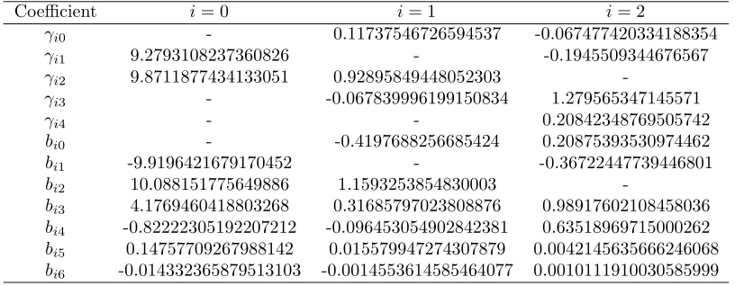
tolerance, set to 10−6. The resultant values forφ
1−φ4 can be found in Table
20
φ1 φ2 φ3 φ4
[image:19.595.109.522.182.341.2]0.3319 0.1932 1.7329 0.0485
Table 1: Optimisation output
Coefficient i= 0 i= 1 i= 2
γi0 - 0.11737546726594537 -0.067477420334188354
γi1 9.2793108237360826 - -0.1945509344676567
γi2 9.8711877434133051 0.92895849448052303
-γi3 - -0.067839996199150834 1.279565347145571
γi4 - - 0.20842348769505742
bi0 - -0.4197688256685424 0.20875393530974462
bi1 -9.9196421679170452 - -0.36722447739446801
bi2 10.088151775649886 1.1593253854830003
-bi3 4.1769460418803268 0.31685797023808876 0.98917602108458036
bi4 -0.82222305192207212 -0.096453054902842381 0.63518969715000262
bi5 0.14757709267988142 0.015579947274307879 0.0042145635666246068
bi6 -0.014332365879513103 -0.0014553614585464077 0.0010111910030585999
Table 2: Optimised boundary coefficients appearing in section 2.
4.1. Composite Template Modified Wavenumber Characteristics
1
The coupled modified wavenumber properties of a composite template are 2
dependent on the number of grid points we choose to analyse. To precisely 3
represent its resolution characteristics we would need to include the effect 4
of every grid point we plan to use in our simulation. Clearly this becomes 5
impractical for simulations of any meaningful size due to cost constraints. 6
For this reason optimisations are based on the simplest scenario, a 7 by 7 7
matrix system consisting of 3 boundary schemes on either side of the domain 8
and 1 central interior point. Additionally since the modified wavenumber 9
characteristics of the template will be symmetrical about the centre point we 10
will only analyse the first 4 points. Although this is the most fundamental 11
system we can examine it is found to be more than sufficient at demonstrating 12
producing substantial accuracy gains in section 5. 1
0 0.2 0.4 0.6 0.8 1 10−6
10−5 10−4 10−3 10−2 10−1 100 101
ω/π
ǫR
(
ω
)
i= 0
New Kim [1]
0 0.2 0.4 0.6 0.8 1 ω/π
i= 1
New Kim [1]
0 0.2 0.4 0.6 0.8 1 ω/π
i= 2
[image:20.595.114.488.155.274.2]New Kim [1]
Figure 1: Real wavenumber errors produced by the the new finite difference template and that of Kim [1] at the three boundary nodes (i= 0,1,2) based on aN = 7 matrix system
0 0.2 0.4 0.6 0.8 1 10−6
10−5 10−4 10−3 10−2 10−1 100 101
ω/π
ǫI
(
ω
)
i= 0
New Kim [1]
0 0.2 0.4 0.6 0.8 1 ω/π
i= 1
New Kim [1]
0 0.2 0.4 0.6 0.8 1 ω/π
i= 2
New Kim [1]
Figure 2: Imaginary wavenumber errors produced by the the new finite difference template and that of Kim [1] at the three boundary nodes (i= 0,1,2) based on a N = 7 matrix system
Since the resolution properties of each point in Eq.(8) are coupled, it 2
is possible that optimising one point in the composite template can have 3
a detrimental effect on others. For this reason resolution errors tend to 4
be higher than if each scheme were analysed individually. This makes it 5
very hard to draw comparisons between resolution errors obtained in studies 6
based on a decoupled approach. Consequently comparisons are made with 7
[image:20.595.113.487.340.462.2]0 0.2 0.4 0.6 0.8 1 10−6
10−5 10−4 10−3 10−2 10−1 100 101
ω/π
ǫR
(
ω
)
i= 0
N= 7
N= 9
N= 11
0 0.2 0.4 0.6 0.8 1 ω/π
i= 1
0 0.2 0.4 0.6 0.8 1 ω/π
[image:21.595.114.488.129.250.2]i= 2
Figure 3: Real wavenumber errors produced by the the new finite difference template at the three boundary nodes (i = 0,1,2) with an increasing number of points analysed (N = 7,9,11)
0 0.2 0.4 0.6 0.8 1 10−6
10−5 10−4 10−3 10−2 10−1 100 101
ω/π
ǫI
(
ω
)
i= 0
N= 7
N= 9
N= 11
0 0.2 0.4 0.6 0.8 1 ω/π
i= 1
0 0.2 0.4 0.6 0.8 1 ω/π
[image:21.595.113.490.315.436.2]i= 2
Figure 4: Imaginary wavenumber errors produced by the the new finite difference template at the three boundary nodes (i = 0,1,2) with an increasing number of points analysed (N = 7,9,11)
0 0.2 0.4 0.6 0.8 1 10−6
10−5 10−4 10−3 10−2 10−1 100 101
ω/π
ǫR
(
ω
)
i= 3,N= 7
New Kim [1]
0 0.2 0.4 0.6 0.8 1 ω/π
i= 3,N= 9
0 0.2 0.4 0.6 0.8 1 ω/π
i= 3,N= 11
[image:21.595.112.489.499.623.2]0 0.2 0.4 0.6 0.8 1 10−6
10−5 10−4 10−3 10−2 10−1 100 101
ω/π
ǫI
(
ω
)
i= 3,N= 9
New Kim [1]
0 0.2 0.4 0.6 0.8 1 ω/π
[image:22.595.177.436.125.249.2]i= 3,N= 11
Figure 6: Imaginary wavenumber error produced by the the new finite difference template and that of Kim [1] at the first interior node (i= 3) with N = 9 and N = 11. N = 7 is not shown as the dissipation error is zero due to the i= 3 being located at the centre of the composite template.
and 2 describe the respective dispersion and dissipation properties produced 1
by Kim’s template and the current study. Differences between ω and ¯ω at 2
each nodal point i are measured by means of a relative error for both real 3
and imaginary components [1]: 4
ǫR,i(ω) =
Re( ¯ωi)−ω ω
(23)
ǫI,i(ω) =
Im( ¯ωωi)
(24)
The wavenumber range for which the dispersion and dissipation errors are 5
below a specified tolerance σ, can be identified by the critical wavenumbers 6
ωσ
Rc,i and ωIc,iσ , such thatǫR,i < σ for 0≤ω ≤ωRc,iσ and ǫI,i < σ for 0≤ω ≤ 7
ωσ
Ic,i, with 0≤ω ≤π. Table 3 shows a comparison of the critical wavenum-8
bers attained using σ = 0.01,0.05 and 0.1. Overall the newly optimised 9
template offers greatly reduced resolution errors. The only exception is the 10
0.41≤ω ≤0.61. This occurs because the objective function (Eq.(13)) aims 1
to reduce the resolution error of the composite template as a whole. In the 2
case of the i= 2 scheme this results is some increase to the dissipation error 3
relative to Kim’s scheme [1], but a more substantial reduction to dispersion 4
error. 5
Figures 3 and 4 show the influence of the number of grid points (N) used 6
in the modified wavenumber analysis on the boundary scheme dispersion and 7
dissipation errors. Each matrix system implements 6 boundary nodes, and an 8
increasing number of interior nodes (N−6). The wavenumber errors quickly 9
converge as N is increased, with only small changes observed between the 10
N = 7 and N = 9,11 cases. 11
Although the coefficients of the first interior point is fixed its resolution 12
properties will be altered by the adjacent boundary schemes due to the fully 13
coupled nature of the modified wavenumber formulation. Figure 5 shows the 14
dispersion error of the new template and that of Kim [1] obtained at thei= 3 15
node with increasing values of N. For N = 7 the new template offers some 16
improvement to the critical wavenumber based on the stricterσ = 0.01 error 17
tolerance. AsN increases a much larger improvement is revealed. AtN = 11 18
the new schemes achieve a critical wavenumber of ω0.01
Rc,3 = 0.651π compared
19
to 0.277π for those of Kim [1]. This highlights how the reductions made to 20
the resolution error at the boundaries has a positive knock-on effect at the 21
near boundary interior nodes. The dissipation errors for the i = 3 node are 22
compared in Figure 6 for N = 9 and N = 11. (N = 7 is not included in 23
this case as its dissipation error is zero due to the i= 3 node being located 24
the new template obtains an improved critical wavenumber ofω0.01
Ic,3 = 0.593π
1
compared to 0.341π for the template of Kim [1]. 2
New schemes Kim [1]
σ= 0.01 σ= 0.05 σ= 0.1 σ= 0.01 σ= 0.05 σ= 0.1
ωσ
Rc,0 0.223π 0.269π 0.306π 0.123π 0.203π 0.308π
ωσ
Ic,0 0.142π 0.217π 0.504π 0.134π 0.183π 0.210π
ωσ
Rc,1 0.354π 0.534π 0.565π 0.174π 0.267π 0.342π
ωσ
Ic,1 0.219π 0.593π 0.623π 0.207π 0.278π 0.317π
ωσ
Rc,2 0.319π 0.660π 0.703π 0.217π 0.329π 0.398π
ωσ
Ic,2 0.307π 0.566π 0.609π 0.373π 0.518π 0.610π
ωσ
[image:24.595.140.466.176.290.2]Rc,3 0.293π 0.579π 0.626π 0.247π 0.626π 0.662π
Table 3: Critical wavenumbers obtained by the the new template and that of Kim [1] based on anN = 7 matrix system at thei= 0,1,2 and 3 nodes utilising various tolerances (σ)
4.2. Stability Analysis
3
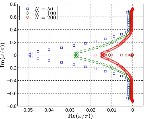
As shown in Table 1 the outcome of the GA stability constraint for the 4
filter cut-off was the boundary weighting factorw2 = 0.0485. The eigenvalue
5
distribution for these settings is shown in Figure 7. As desired the real parts 6
of all eigenvalues have been restricted into the left half plane. The optimised 7
boundary weighting obtains stable eigenvalues over the filter cut-off range 8
0.74π ≤ Ωc ≤ 0.88π, despite the constraint focusing only on the upper 9
stability limit Ωc = 0.88π. If a lower cut-off value is desired a stable solution 10
can still be obtained by reverting to the default value w2 = 0.085. In order
11
to obtain the largest magnitude negative real eigenvalues over the longest 12
stability range the authors suggest implementing the following strategy for 13
w2
−0.05 −0.04 −0.03 −0.02 −0.01 0 −0.8
−0.6 −0.4 −0.2 0 0.2 0.4 0.6 0.8
Re(ω/π))
Im
(
ω
/
π
))
N = 50
N = 100
[image:25.595.172.425.135.343.2]N = 200
Figure 7: Eigenvalues at various grid sizes for the newly optimised finite difference template with compact filtering
w2 =
0.0850 for 0.59π ≤Ωc <0.86π,
0.0485 for 0.86π ≤Ωc ≤0.88π.
(25)
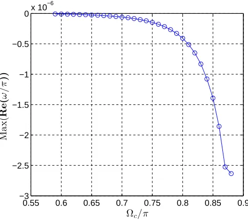
By adopting this strategy a stable eigenvalue distribution is attainable 1
over the filter cut-off range 0.59π ≤ Ωc ≤ 0.88π. Figure 8 shows the maxi-2
mum real eigenvalues obtained over this range utilising both weighting factors 3
accordingly. 4
A more extensive stability analysis can be preformed through application 5
of a test function to a scalar linear wave convection problem, again described 6
by Eq.(18). In this particular instance a modulated wave described by the 7
0.55 0.6 0.65 0.7 0.75 0.8 0.85 0.9 −3
−2.5 −2 −1.5 −1 −0.5
0x 10
−6
Ωc/π
M
a
x
(
R
e
(
ω
/
π
[image:26.595.186.428.129.344.2]))
Figure 8: Maximum real eigenvalues for the new schemes with compact filtering over the stable range 0.59π≤Ωc ≤0.88π. (w2 = 0.0485 for 0.86π≤Ωc ≤0.88π andw2= 0.085
for 0.59π≤Ωc <0.85π)N = 200
f(x, t= 0) =f∞
1 +Acos
k1x
L
sin
k2x
L
, (26)
f(x= 0, t) =f∞
1 +Acos
−c∞k1t
L
sin
−c∞k2t
L
. (27)
Here the frequency and amplitude of the carrier wave component are 1
represented by k2 = 25k1 and f∞ respectively. Equivalently, k1 = 2π and
2
A = 1.5 represent the frequency and amplitude of the modulating component. 3
The boundary schemes are implemented at both the inlet and outlet to the 4
domain. To obtain the exact solution to this problem x is substituted for 5
ˆ
x=x−c∞tin Eq.(26). Stability of the new template and filters is tested by 6
101 102 103 104
10−4
10−3
10−2
10−1
100
N
M
ea
n
Eℓ
2
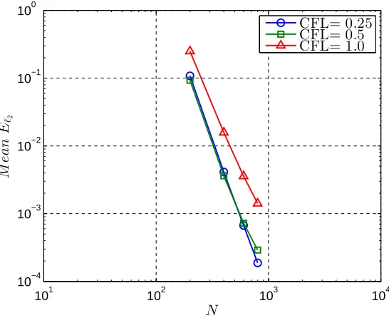
[image:27.595.164.437.136.359.2]CFL= 0.25 CFL= 0.5 CFL= 1.0
Figure 9: Meanℓ2-norm errors produced by the current schemes in calculation of a
mod-ulated linear wave for CFL=0.25, CFL=0.5 and CFL=1.0
coarser grid sizes the calculation is continued untilt= 150L/c∞, while for the 1
finest grid (N = 800) it is run until t = 10L/c∞ to minimise computational 2
cost. Temporal discretisation is achieved with classical 4th order Runge-3
Kutta. To quantify numerical errors the following ℓ2-norm error is defined:
4
Eℓ2 = ( N
X
i=1
[fi−fexact]2/(Nf∞2)
)1 2
(28)
Figure 9 shows the time averaged ℓ2-norm errors produced during calculation
5
of the linear modulated wave for various CFL numbers. Stable solutions with 6
4.3. Comparison to Classical Methods
1
The accuracy enhancements made available by utilising pentadiagonal 2
compact schemes including the newly optimised boundaries is shown in Fig-3
ure 10. It displays the ℓ2-norm error time history (Eq.(28)) obtained during
4
calculation of a 1D linear scalar wave convection problem utilising different 5
spatial discretisation schemes and N = 400 grid cells. Temporal discretisa-6
tion is conducted with classical 4th order Runge-Kutta with a value of 0.5 7
for the Courant-Friedrichs-Lewy condition (CFL). A full description of this 8
problem is given in section 5.1. The classical explicit method (4th order 9
central interior and 3rd order boundaries) is capable of obtaining a stable 10
solution, albeit with a very large peak error. This highlights the requirement 11
for grid refinement in order to obtain a more acceptable accuracy, inevitably 12
increasing the computational cost. Adopting an implicit method can be an 13
effective way to reduce the level of error for a given grid spacing. This is ap-14
parent over the regiontc∞/L < 0.4, where the standard 4th order tridiagonal 15
Pad´e scheme, used here with 2nd order implicit boundaries [17] achieves no-16
tably better performance. However such methods often suffer from stability 17
issues, as shown by the divergence at a later time step. This demonstrates 18
the requirement for scheme optimisation to achieve higher levels of accuracy 19
and computational efficiency, without neglecting numerical stability. In the 20
case of the current pentadiagonal system, error reductions in excess of two 21
orders of magnitude are achieved relative to the explicit method, while still 22
0 0.25 0.5 0.75 1 1.25 1.5
10−6
10−4
10−2
tc∞/L Eℓ
2
New
[image:29.595.160.438.255.474.2]Pad´e (4th-order interior+2nd-order boundary [17]) Explicit (4th-order interior+3rd-order boundary)
Figure 10: Comparison of ℓ2-norm error time histories obtained during the 1D scalar
5. Benchmark Problems
1
5.1. One-dimensional Scalar Wave
2
The first benchmark problem we consider is the convection of a one-3
dimensional scalar wave. This problem was first proposed by Tam [18] at the 4
Fourth Computational Aeroacoustics Workshop on Benchmark Problems. It 5
consists of the simulation of a wave pulse as it travels from its initial location 6
within the domain through a computational exit boundary. Unlike the wave 7
convection problem used to analyse the long term linear stability of the finite 8
difference schemes in section 4, the wave in this problem will entirely leave 9
the domain, resulting in a final solution of zero. This allows us to analyse 10
the capability of the proposed schemes at minimising error reflections at 11
computational boundaries. The initial wave pulse is defined as 12
−0.5 −0.4 −0.3 −0.2 −0.1 0 0.1 0.2 0.3 0.4 0.5 0.6 0.7 0.8 0.9 1
−0.5 0 0.5 1 1.5 2 2.5 3
x/L
f
/
f∞
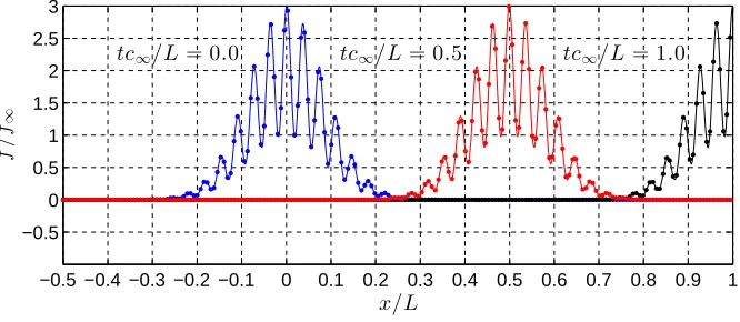
[image:30.595.133.466.413.558.2]tc∞/L= 0.0 tc∞/L= 0.5 tc∞/L= 1.0
Figure 11: 1D scalar wave at three instances of time — = exact solution,• = numerical solution for N = 1000 and CFL=0.5
f(x, t= 0) =f∞
2 + cos
k1x
L
exp
−k2ln(2)x
2
L2
where k2 = 100 andk1 = 1.7k2. The wave is convected via Eq.(18) over the
1
range −0.5L≤x≤L. The exact solution is obtained by 2
fexact(x, t) =f∞
2 + cos
k1xˆ
L
exp
−k2ln(2)ˆx
2
L2
(30)
where ˆx = x−c∞t. Since the wave pulse is initialised within the domain, 3
nothing will pass through the inlet boundary. For this reason the interior 4
schemes can be applied at the inlet boundary points (i={0,1,2}) with the 5
following boundary condition [1]: 6
f(x <−0.5L, t) =f′(x <
−0.5L, t) = 0 for t≥0 (31)
0 0.25 0.5 0.75 1 1.25 1.5
10−8
10−7
10−6
10−5
10−4
tc∞/L Eℓ
2
[image:31.595.161.437.375.603.2]New Kim [1] Liu [11] Jordan [13]
Figure 12: Time history of ℓ2-norm error produced by various schemes in calculation of
the 1D scalar wave,N = 1000, CFL=0.5
boundary nodes (i = {N, N − 1, N − 2}) by measuring the error as the 1
wave pulse leaves the domain at the non-dimensional time tc∞/L= 1.0. Er-2
rors produced by the current schemes are compared to those produced by the 3
schemes of Kim [1], Jordan [13] and Liu et al. [11]. Results are firstly pre-4
sented without the assistance of compact filters, then comparisons are made 5
to their filtered counterparts, thus demonstrating each templates sensitivity 6
to the filtering process. The newly optimised schemes use the new boundary 7
weighting factors suggested in section 4.2 with a filter cut-off of Ωc = 0.88π, 8
while the other schemes maintain the original filter coefficients suggested in 9
[16]. 10
102 103 104
10−7
10−6
10−5
10−4
10−3
10−2
10−1
N Eℓ
2
[image:32.595.112.486.144.581.2]4th order New Kim [1] Liu [11] Jordan [13]
Figure 13: Maximum ℓ2-norm errors produced in the 1D scalar wave convection problem
by various schemes at different grid levels, CFL=0.5
Figure 11 shows a comparison of the wave produced by the current 11
[image:32.595.161.436.359.583.2]and N = 1000. The numerical result contains no perceivable errors, even as 1
the wave leaves the domain exit boundary at tc/L= 1.0. Figure 12 show the 2
time histories of the ℓ2-norm error at a grid size ofN = 1000. The present
3
schemes exclusively exhibit no overshoot as the wave leaves the domain. This 4
corresponds to peak error reductions of 38.4%, 66.1% and 84.1% compared 5
to that produced by the coefficients of Kim [1], Jordan [13] and Liu et al. 6
[11], respectively. Another important quality, particularly for aeroacoustic 7
simulations is that the final error tends to zero after the wave has left the 8
domain. In this regard the result provided by the current schemes again out-9
performs that of previous studies resulting in a final error reduction of 97.8% 10
compared to Kim [1], 98.9% compared to Jordan [13] and 96.9% compared 11
to Liu et al. [11]. Figure 13 shows the maximum ℓ2-norm errors produced
12
by each scheme at various grid levels. This confirms that the new schemes 13
maintain the desired fourth-order convergence rate, while also achieving the 14
lowest errors on all grid levels. 15
A Comparison between the ℓ2-norm error histories produced with and
16
without compact filtering is shown in Figure 14 forN = 1000. After filtering 17
a comparable peak error level is achieved by the newly optimised schemes, 18
Kim’s schemes and Jordan’s schemes. Liu’s schemes on the other hand still 19
manifests a significant overshoot at tc∞/L = 1.0. The most robust perfor-20
mance is attained by the new schemes, which maintain similar error levels 21
with and without filtering. In fact, they are the only schemes for which the 22
peak error is slightly increased by filtering, suggesting that they are success-23
ful in resolving a broader range of scales. Conversely the schemes of Kim and 24
0 0.25 0.5 0.75 1 1.25 1.5
10−9
10−8
10−7
10−6
10−5
10−4
tc∞/L
Eℓ
2
Jordan [13,16]
Unfiltered
Filtered
0 0.25 0.5 0.75 1 1.25 1.5
10−9
10−8
10−7
10−6
10−5
10−4
tc∞/L
New
Unfiltered
Filtered
0 0.25 0.5 0.75 1 1.25 1.5
10−9
10−8
10−7
10−6
10−5
10−4
Liu [11,16]
Unfiltered
Filtered
0 0.25 0.5 0.75 1 1.25 1.5
10−9
10−8
10−7
10−6
10−5
10−4
Eℓ
2
Kim [1,16]
Unfiltered
[image:34.595.131.462.220.531.2]Filtered
Figure 14: Comparison between ℓ2-norm error histories with and without filtering, N =
extra caution should be exercised while selecting the filter cut-off wavenum-1
ber. The maximum ℓ2-norm errors produced by the new schemes with and
2
without filtering is shown in Figure 15. Demonstrating that the similarity 3
between filtered and unfiltered solutions is consistent over a range of grid 4
levels. 5
102 103 104
10−7
10−6
10−5
10−4
10−3
10−2
10−1
N Eℓ
2
[image:35.595.163.439.246.473.2]4th order New unfiltered New filtered
Figure 15: Comparison of maximumℓ2-norm errors produced in the 1D scalar wave
con-vection problem by the current scheme, with and without filtering, CFL=0.5
5.2. Two-dimensional Inviscid Vortex Convection
6
In this problem the 2D compressible Euler equations are solved in full 7
conservative form, in order to simulate the convection of an inviscid 2D vor-8
ticity wave in a supersonic flow. This problem was originally proposed by 9
The governing equations are described as follows 1 ∂Q ∂t + ∂E ∂x + ∂F
∂y =0, (32)
where Q, E and F represent the following: 2 Q= ρ ρu ρv ρet
, E=
ρu
ρu2+p
ρuv
ρ(et+p)u
and F=
ρv ρuv
ρv2+p
ρ(et+p)v . (33)
where ρ,u, v and pare the primitive variables (density, streamwise velocity, 3
vertical velocity and pressure), and subscript∞represents free-stream condi-4
tions. The total energy per unit mass is given byet=p/[(γ−1)ρ]+(u2+v2)/2,
5
and γ =cp/cv is the ratio of specific heats, set to γ = 1.4 for air. The calcu-6
lation is carried out with the following initial conditions 7
ρ(x, y) ρ∞
=
1− γ−1
2 ψ
2(x, y) 1
γ−1
u(x, y) a∞
=M∞+Kyψ(x, y)
v(x, y) a∞
=−Kxψ(x, y)
p(x, y) p∞ = ρ ρ∞ γ , for
−0.5L≤x≤2.5L
−0.75L≤y≤0.75L,
with 1
ψ(x, y) = ǫ 2πexp
1
2(1−K
2(x2+y2))
, (35)
where K = 1/R and R = 0.08L, which represents the radius of the vortex. 2
The vortex strength is controlled by the parameter ǫ. ǫ = 0.1 corresponds 3
to a linear case, while higher values correspond to more non-linear cases. 4
The free stream velocity is defined as u∞ =M∞a∞, with the Mach number 5
M∞ = 2, and the ambient speed of sound a∞ =
p
γp∞/ρ∞. As there 6
is a supersonic free stream velocity, downstream disturbances will have no 7
influence on upstream flow properties. Therefore boundary conditions need 8
not be applied at the domain outlet. Furthermore this advocates the use 9
of interior schemes at the first three inlet boundary points, since the x-10
derivatives in Eq.(32) may be set to zero prior the inlet boundary. In addition 11
to the domain outlet, boundary schemes are applied to the top (j = {N − 12
2, N −1, N}) and bottom edges (j = {0,1,2}) of the grid with the non-13
reflective boundary conditions suggested in [20]. The compact filter cut-off 14
frequency of Ωc = 0.88πis used with the boundary weighting factors to ensure 15
a numerical stable solution is obtained. As before time integration is carried 16
out with classical fourth-order Runge-Kutta method, until a non-dimensional 17
time of u∞t/L= 1.5 using CFL=0.5. 18
In order to identify the errors generated at the exit boundary the solu-19
tion generated on the domain −0.5L ≤ x ≤ 2.5L, −0.75L ≤ y ≤ 0.75L is 20
treated as a reference solution. This is compared to the result obtained on a 21
grid truncated by a factor of 2 in the streamwise direction (−0.5L≤x≤L, 22
−0.75L ≤ y ≤ 0.75L). At u∞t/L = 1.0 the core of the propagating vortex 23
within the interior region of the full length domain. By comparing solutions 1
at this instant of time the accuracy of the boundary schemes can be deter-2
mined. Further justification for this approach is provided in Appendix A. 3
A two-dimensional equivalent of the ℓ2-norm error, based on corresponding
4
grid points of the truncated and full length domains can be defined as follows 5
Eℓ2(ts) = L
2
[(N + 1)ǫu∞]2
N X
i=0
N X
j=0
(νi,jF −νi,jT )2 !1/2
(36)
x/L
y/
L
-0.5 0 0.5 1
-0.5 0 0.5
u∞t/L=0.0 u∞t/L=0.5 u∞t/L=1.0
x/L
y/
L
0.8 0.85 0.9 0.95 1 1.05 1.1 1.15 1.2
-0.2 -0.15 -0.1 -0.05 0 0.05 0.1 0.15
0.2 p/(
∞a
2
∞)
[image:38.595.118.498.249.484.2]0.70 0.65 0.60 0.55 0.50 0.45 0.40 0.35 0.30 0.25 0.20
Figure 16: Left: Contours of normalised pressure for the vortex convection problem ob-tained by the new schemes at three instances of time withǫ= 5. The domain is truncated by a factor of 2 in the streamwise direction such that a computational exit boundary exists at x= 1.0L, where boundary schemes are applied. A total of 60×60 grid cells are used for the computation with a uniform grid spacing of ∆x= 0.025L. Right: Comparison of normalised pressure contours aroundx= 1.0Lfor the truncated domain and a full length domain where the exit boundary is further downstream. The full length domain maintains the same grid spacing and hence consists of 120×60 grid cells
where ν is a normalised primitive variable (u/a∞, v/a∞, ρ/ρ∞, p/(ρ∞a2∞)), 6
(N + 1)2 is the number of grid points contained within the truncated grid,
7
length and truncated domains. All numerical errors are compared to those 1
produced using the coefficients suggested by Kim [1, 16]. 2
Figure 16 show contours of normalised pressure obtained at three in-3
stances of time u∞t/L= 0,0.5,1.0 on a truncated 60×60 grid. There are no 4
observable deformations as the vortex leaves the exit boundary at x= 1.0L. 5
Also shown is a comparison of the solution produced on both the truncated 6
(60×60 grid) and reference grids (120×60 grid) atu∞t/L= 1.0. Despite the 7
fact that this result is obtained on a very coarse grid with the most non-linear 8
vortex strength (ǫ= 5), the two results remain consistent. 9
101 102 103 104
10−14 10−13 10−12 10−11 10−10
10−9
10−8
10−7
10−6
10−5
10−4
10−3
N Eℓ
2
o
f
p
/
(
ρ∞
a
2 )∞
[image:39.595.175.437.338.558.2]4th Order ǫ= 5 ǫ= 3 ǫ= 1 ǫ= 0.1
Figure 17: ℓ2-norm errors based on p/(ρ∞a 2
∞) produced at u∞t/L = 1.0 by the new
schemes during the vortex convection problem. Results shown with ǫ= 0.1,1,3 and 5 at various grid levels
Figure 17 shows the convergence rates of the normalised pressure ℓ2
-10
level the grid spacing is kept uniform in both the streamwise and vertical 1
directions. The current schemes successfully exceed the desired fourth-order 2
convergence rate for both linear and non-linear vortex cases. Comparisons 3
to the previous study [1, 16] are also given in Figure 18 for each primitive 4
variable and ǫ= 5. Large error reductions are achieved by the new schemes
101 102 103 104
10−13
10−12
10−11
10−10
10−9
10−8
10−7
10−6
10−5
10−4
10−3
N
Eℓ
2
ρ/ρ∞
4th Order New Kim [1,16]
101 102 103 104
10−13
10−12
10−11
10−10
10−9
10−8
10−7
10−6
10−5
10−4
10−3
N p/(ρ∞a2∞)
4th Order New Kim [1,16]
101 102 103 104
10−13
10−12
10−11
10−10
10−9
10−8
10−7
10−6
10−5
10−4
10−3
v/a∞
4th Order New Kim [1,16]
101 102 103 104
10−13
10−12
10−11
10−10
10−9
10−8
10−7
10−6
10−5
10−4
10−3
Eℓ
2
u/a∞
[image:40.595.112.491.238.588.2]4th Order New Kim [1,16]
Figure 18: Primitive variableℓ2-norm errors generated by the new schemes and those of
Kim [1, 16] during the vortex convection problem with an increasing number of nodes. Errors calculated atu∞t/L= 1.0 with ǫ= 5
5
of magnitude. On average errors are reduced by a factors of 8.31,7.72,5.42 1
and 8.58 for u/a∞, v/a∞, ρ/ρ∞ and p/(ρ∞a2∞) respectively across the five 2
grid levels tested. This clearly demonstrates that the present schemes are 3
also capable of large accuracy improvements in multidimensional problems. 4
Further comparisons for the error based on normalised pressure are shown 5
in Figure 19 foru∞t/L = 1.0 obtained with different vortex strengths. Using 6
a 60×60 grid error reductions range from 60.1%−82.2%, while for a 300×300 7
grid they fall between 88.6% −91.3%. In Figure 20 comparisons are also 8
made with the schemes of Liu et al. [11] and Jordan [13] for the error time 9
history using a 60×60 grid and ǫ = 5. For each case compact filtering is 10
employed to ensure stable solutions. The results are shown firstly with a filter 11
cut-off of Ωc = 0.88π utilising the boundary weighting strategy in Eq.(17). 12
The new schemes are successful in obtaining the lowest errors during the 13
simulation. A similar performance is also achieved for the schemes of Jordan 14
[13], however as demonstrated in the previous one-dimensional benchmark 15
problem the low errors produced by Jordan’s template were not maintained 16
when the filter cut-off was increased. With a higher filter cut-off (globally set 17
to Ωc = 0.95π) the error produced by Jordan’s schemes increases, whereas 18
for the new schemes it is reduced, thus resulting in a more substantial error 19
reduction offered by the new schemes. 20
5.3. Deformed Grid Two-dimensional Inviscid Vortex Convection
21
In this benchmark problem the performance of the current schemes on 22
curvilinear grids is analysed by revisiting the two-dimensional inviscid vortex 23
convection problem. The original uniform grid is deformed by implementing 24
0 1 2 3 4 5
10−7
10−6
10−5
10−4
ǫ
Eℓ
2
of
p
/
(
ρ∞
a
2)∞
(N×N) = (60×60)
New Kim [1,16]
0 1 2 3 4 5
10−11
10−10
10−9
10−8
ǫ
Eℓ
2
of
p
/
(
ρ∞
a
2 )∞
[image:42.595.114.499.154.305.2](N×N) = (300×300)
Figure 19: Comparison ofℓ2-norm errors based onp/(ρ∞a 2
∞) produced during the vortex
convection problem. Obtained at u∞t/L = 1.0, with various vortex strengths (ǫ). Left:
60×60 grid. Right: 300×300 grid
0.7 0.8 0.9 1 1.1 1.2 1.3
2 4 6 8
10x 10
−5
u∞t/L
Eℓ
2
of
p/
(
ρ∞
a
2)∞
Ωc= 0.88π
New Kim [1,16] Liu [11,16] Jordan [13,16]
0.7 0.8 0.9 1 1.1 1.2 1.3
2 4 6 8
10x 10
−5
u∞t/L
Ωc= 0.95π
Figure 20: Time history ofℓ2-norm errors based onp/(ρ∞a 2
∞) produced during the vortex
convection problem withN×N = 60×60 andǫ= 5. Left: filter cut-off Ωc= 0.88πutilising
the boundary weighting strategy in Eq.(17) (w2 = 0.085 previous schemes, w2 = 0.0485
[image:42.595.123.487.426.583.2]xi,j =−L 2 +
3L 2
i
N +µsin
4πj N
yi,j =−3L
4 +
3L 2
j
N +µsin
4πi N
(37)
where µ determines the amount of grid deformation. µ = 0 would revert 1
the grid to the uniform case analysed in the previous section. As before the 2
problem consists of solving the compressible two-dimensional Euler equa-3
tions, although this time in a generalised coordinate system 4
∂Qb
∂t +
∂Eb
∂ξ +
∂Fb
∂η =0, (38)
with 5
b
Q=Q/J, Eb = (ξxE+ξyF)/J, Fb = (ηxE+ηyF)/J (39)
whereξx,y andηx,y are the grid metrics, andJ−1 = (xξyη =xηyξ) is the
Jaco-6
bian determinant of the transformation. Since the finite-difference template 7
is also required to calculate the grid metric this represents a more thorough 8
test of their performance. The calculations are run using the most non-linear 9
vortex case (ǫ = 5), CF L= 0.5, and M∞ = 2.0. The compact filtes are also 10
implemented utilising Ωc = 0.88π and the appropiate boundary weighting 11
factors. The ℓ2 norm errors are once again evaluated based on Eq.(36) as
12
the vortex leaves the exit boundary at x= 1.0L. Figure 21 shows contours 13
on normalised spanwise vorticity (ωzL/(a∞ǫ) whereωz =∂v/∂x−∂u/∂y) at 14
three instances of time (u∞t/L= 0,0.5 and 1.0). The truncated domain grid 15
points shown). At u∞t/L= 1.0 the vortex is halfway through the truncated 1
domain exit boundary. At this point there is no noticable deformation to the 2
vortex or disimilarity with the full domain solution. 3
-0.5 0 0.5 1 1.5
-1 -0.5 0 0.5 1
|
ω
z|L/(a
∞ε
)
6.6 6 5.4 4.8 4.2 3.6 3 2.4 1.8 1.2 0.6 0
x/L
y/
[image:44.595.165.453.220.439.2]L
Figure 21: Contours of normalised spanwise vorticity magnitude for the vortex convection problem utilising a curvilinear (deformed) grid. The grid (generated by Eq.(37)) consists of 100×100 grid cells with a uniform spacing andµ= 0.05 (1 in 2 grid lines shown)
The maximumℓ2norm error convergence is shown in Figure 22 for the new
4
schemes and those of Kim [1, 16] based on normalised pressure (p/(ρ∞a2∞). 5
This demonstrates that the new schemes are able to maintain the desired 6
4th-order convergence rate on heavily deformed curivlinear grids. The er-7
ror reduction produced by the new schemes increases with N ranging from 8
52.16% for the coarsest grid, to 94.63% for the finest. Figure 23 shows the ℓ2
9
norm error time history produced by the new schemes and those of Kim [1], 10
with the compact filtering [16], with results shown for the 100×100 grid. The 1
new schemes achieve a 12.6, 7.2 and 3.0 times improvement to the maximum 2
error produced during the calculation compared to the schemes of Liu et al. 3
[11], Kim [1] and Jordan [13] respectively. 4
101 102 103
10−10
10−9
10−8
10−7
10−6
10−5
10−4
10−3
N Eℓ
2
o
f
p
/
(
ρ∞
a
2 )∞
[image:45.595.176.437.232.453.2]4th Order New Kim [1,16]
Figure 22: ℓ2-norm errors based on p/(ρ∞a 2
∞) produced at u∞t/L = 1.0 by the new
schemes and those of Kim [1, 16] during the deformed grid vortex convection problem withµ= 0.05. Results shown withǫ= 5 at various grid levels
6. Pseudo-boundary Schemes
5
Thus far we have concentrated on reducing the total resolution error 6
between the composite template and exact differentiation. Another potential 7
target for improvement is the relative error between consecutive points in the 8
composite template. This is a particular concern between the final central 9
sharp degradation in the spectral properties are observed. The approach 1
taken in this section is to retune the coefficients of the first few interior 2
nodes, such that they ease this performance discontinuity, and thus achieve 3
a higher accuracy. The retuned interior schemes are herein referred to as 4
pseudo-boundary schemes. The coefficient matrices PandQ are updated to 5
include the pseudo-boundary schemes at nodesi={3, N−2},i={4, N−1} 6
and i = {5, N} are displayed below. Hatted variables denote the pseudo-7
boundary coefficients. 8
0.7 0.8 0.9 1 1.1 1.2 1.3
0.5 1 1.5 2
2.5x 10
−5
u∞t/L
Eℓ
2
o
f
p
/
(
ρ∞
a
2 )∞
[image:46.595.176.438.312.536.2]New Kim [1,16] Liu [11,16] Jordan [13,16]
Figure 23: Time history ofℓ2-norm errors based onp/(ρ∞a 2
∞) produced by various schemes
during the deformed grid vortex convection problem using ǫ = 5. The grid consists of
![Figure 1: Real wavenumber errors produced by the the new finite difference template andthat of Kim [1] at the three boundary nodes (i = 0, 1, 2) based on a N = 7 matrix system](https://thumb-us.123doks.com/thumbv2/123dok_us/1563858.109002/20.595.113.487.340.462/figure-wavenumber-produced-nite-dierence-template-andthat-boundary.webp)
![Figure 5: Real wavenumber error produced by the the new finite difference template andthat of Kim [1] at the first interior node (analysed (i = 3) with an increasing number of pointsN = 7, 9, 11)](https://thumb-us.123doks.com/thumbv2/123dok_us/1563858.109002/21.595.114.488.129.250/figure-wavenumber-produced-dierence-template-interior-analysed-increasing.webp)
![Figure 6: Imaginary wavenumber error produced by the the new finite difference templateand that of Kim [1] at the first interior node (not shown as the dissipation error is zero due to thei = 3) with N = 9 and N = 11](https://thumb-us.123doks.com/thumbv2/123dok_us/1563858.109002/22.595.177.436.125.249/figure-imaginary-wavenumber-produced-dierence-templateand-interior-dissipation.webp)
![Table 3: Critical wavenumbers obtained by the the new template and that of Kim [1]based on an N = 7 matrix system at the i = 0, 1, 2 and 3 nodes utilising various tolerances(σ)](https://thumb-us.123doks.com/thumbv2/123dok_us/1563858.109002/24.595.140.466.176.290/table-critical-wavenumbers-obtained-template-utilising-various-tolerances.webp)
![Figure 10: Comparison of ℓexplicit finite difference scheme with 3rd order explicit boundaries, a classical 4th orderPad´e scheme with 2nd order implicit boundaries [17], and the current numerical setup.The simulation is conducted withwave convection problem](https://thumb-us.123doks.com/thumbv2/123dok_us/1563858.109002/29.595.160.438.255.474/comparison-explicit-dierence-boundaries-boundaries-simulation-conducted-convection.webp)