Robust artificial neural network for reliability and sensitivity analysis of complex non-linear systems

Robust Artificial Neural Network for Reliability and

Sensitivity Analysis of Complex Non-Linear Systems

Uchenna Oparajia,b, Rong-Jiun Sheub, Mark Bankheadc, Jonathan Austinc, Edoardo Patellia,∗

a_{Institute for Risk and Uncertainty, University of Liverpool, Chadwick Building, Peach}

Street, Liverpool L69 7ZF, United Kingdom

b_{Institute of Nuclear Engineering and Science, National Tsing Hua University, Hsinchu,}

Taiwan

c_{National Nuclear Laboratory, Chadwick House, Warrington Rd, Birchwood Park,}

Warrington, Cheshire, WA3 6AE, United Kingdom

Abstract

Artificial Neural Networks (ANNs) are commonly used in place of expensive models to reduce the computational burden required for uncertainty quan-tification, reliability and sensitivity analysis. ANN with selected architecture is trained with the back-propagation algorithm from few data representatives of the input/output relationship of the underlying model of interest. How-ever, different performing ANNs might be obtained with the same training data as a result of the random initialization of the weight parameters in each of the network, leading to an uncertainty in selecting the best performing ANN. On the other hand, using cross-validation to select the best perform-ing ANN based on the ANN with the highest R2 value can lead to biassing in the prediction. This is as a result of the fact that the use of R2 _cannot

determine if the prediction made by ANN is biased. Additionally, R2 does

∗_{Corresponding author}

Email addresses: [email protected](Uchenna Oparaji),

not indicate if a model is adequate, as it is possible to have a low R2 _{for a}

good model and a high R2 for a bad model. Hence in this paper, we propose an approach to improve the robustness of a prediction made by ANN. The approach is based on a systematic combination of identical trained ANNs, by coupling the Bayesian framework and model averaging. Additionally, the uncertainties of the robust prediction derived from the approach are quan-tified in terms of confidence intervals. To demonstrate the applicability of the proposed approach, two synthetic numerical examples are presented. Fi-nally, the proposed approach is used to perform a reliability and sensitivity analysis on a process simulation model of a UK nuclear effluent treatment plant developed by National Nuclear Laboratory (NNL) and treated in this study as a black-box employing a set of training data as a test case. This model has been extensively validated against plant and experimental data and used to support the UK effluent discharge strategy.

Keywords:

Monte-Carlo Simulation, Global Sensitivity Analysis, Reliability Analysis, Artificial Neural Network, Uncertainty Quantification

1. Introduction

in simulating the behaviour of these systems. This advance in computational development has allowed engineering practitioners to reduce the number of expensive test required to qualify a new system/product. On the other hand, a quantifiable mathematical model simulating the performance of a system is viewed to be composed of three main elements such as: 1) an input vector that represents the state variables of the system, 2) a mathematical model defining the system of interest, which is usually seen as a black-box, and finally 3) an output vector that represents the performance of the system. Two types of uncertainties that affects the state variables of the mathematical model are usually considered: 1) randomness due to inherent variability in the system behaviour (aleatory uncertainty) and, 2) imprecision due to lack of knowledge and information on the system (epistemic uncertainty). Usually, the design of complex critical systems requires the explicit consideration of the different levels of uncertainties affecting the state variables of the system for an adequate performance assessment [1, 2].

1.1. Reliability and Sensitivity Analysis for Complex System Performance

Evaluation

To quantify the performance of complex critical systems in the presense of uncertainties, reliability analysis is usally carried out. In mathematical terms, the state variables of a system is defined by a vector collection X =

(X1, X2, ..., Xp) of state variables. The performance criteria of the system

(i.e. limit state) g(X) divides the system state into two regions (i.e. safe domain S = X :g(X)>0 and a failure domain F = X :g(X)≤0). The probability that the system would not meet an expected performance using Monte Carlo method can be expressed as ˆpF = 1/N

PN

indicator functionI(g(Xi)) is 1 ifg(Xi) is negative or 0 otherwise. It should

be noted that among the numerical methods proposed in several literature to estimate ˆpF, simulation methods [3] have attracted significant attention due

to their flexibility and accuracy. Simulation methods are generally applicable to varying systems, but require a balance between computational efficiency and accuracy. These simulation methods includes: Monte Carlo (MC) [4], Importance Sampling [5], Directional Sampling [6], Line Sampling [7, 8], Subset Simulation [9, 10] etc. Each of these simulation methods have special features to target different classes of problems. For instance, in a scenario when the target failure probability ˆpF is less than 10−4, direct Monte Carlo

method [4] is not suited for this problem. Hence, a simulation approach that is suitable for the problem can be adopted (i.e. Subset simulation, Line sampling). Similarly, a system performance can only be improved if the state variables that affect the performance significantly are identified and focused on. Sensitivity analysis is used to achieve this by identifying and ranking the contributions of each state variable of the system to the variability in the performance. Most often, the variance based method to sensitivity analysis [11] is adopted when assessing the contributions of the state variables. This method is a class of simulation approaches that is used to decomposes the output variance into parts that can be attributed to the inputs and interactions between them. The sensitivity indices (i.e. state variable ranking) using this approach are estimated by Si =Vi/V ar(Y) and

Ti = 1−V arX∼i[EX∼i(Y|X∼i)]/V ar(Y), where Si is the contribution of a

single state variable andTi is the contribution due to interactions among the

1.2. Need for Surrogate Models

Unfortunately, reliability and sensitivity analysis using the simulation approach are computationally demanding tasks, requiring a huge number of model runs. To be specific, when performing reliability analysis on a high reliable system with a low failure probability (i.e. pF < 10−4), a huge

number of samplesN is required to accurately compute the failure probability (i.e.N >1/pF). Similarly, when performing sensitivity analysis on a model

with p number of state variables using the variance based method [12], the total number of model evaluations EM follows the relationship EM = (p+

2)N, where N is the number of samples required. The number of samples

N is usually proportional to the dimension of the model being analysed. For instance, Patelli et al., (2012) [13] required greater than 105 _{samples to}

accurately compute the sensitivity indices of the Gravity Field and Steady-State Ocean Circulation Explorer (GOCE) satellite due to the complexity of the finite element (FE) model used (i.e. p > 3000)(see ref [14] also). In a similar fashion, Baroni and Tranola (2014) [15] found out that the sensitivity indices convergence was reached usingN = 1024 samples for a model ofp= 5 uncertain parameters. Generally speaking, the computational cost required for performing the aforementioned analysis can vary amongst different set of models. This is as a result of the time required for a single run of the model. Therefore, to tackle these huge computation restrictions, alternative methods that significantly reduces this computational burden must be sourced out.

1.3. Artificial Neural Networks for Reliability and Sensitivity Analysis

an extremely valuable tool for reducing the computational burden required for performing reliability and sensitivity analysis. For instance, in refs [13, 17–20] ANNs have been used as substitutes to replace expensive models in order to speed up their analysis. The ANNs in the aforementioned literature have been trained with the back-propagation algorithm [21] based on input-output training data set Dtrain(x, y) extracted from the expensive model of

interest. The back-propagation algorithm efficiently computes the slope of the gradient by employing a gradient descent, following the slope of the error function downward along, and simultaneously changing all the weight values of the network. The weight parameters are constantly tuned until the value no longer decreases. However, a limitation of using the back-propagation algorithm to train an ANN is that different performing ANNs (i.e. with identical architecture) arise from the same training data. This is as a result of the gradient decent algorithm used to minimize the error function of an ANN, getting trapped on a different error surface in each ANN. Consequently, cross-validation is utilized to select the best performing ANN in the set by choosing the ANN with the lowest validation regression error (i.e. highest

R2). However, a key limitation of usingR2 to judge the performance of ANN is that it cannot determine whether the weight parameters and predictions of the ANN are biased, as it is possible to have a low R2 value for a good ANN, and a high R2 _{value for an ANN that does not fit the data. Moreover,}

if the validation data is partially corrupted with noise, the evaluation of the

R2 _{will be biased. Hence, we make a claim (see Section 3.2 for verification}

predicted by the selected ANN. Therefore, in this paper, we aim to address this issue by proposing a simple novel approach used to reduce the biasing and improve the robustness of the prediction made by an ANN. The structure of this paper is organized as follows: In Section 2, the proposed approach is discussed. Next, two synthetic numerical examples are presented in Section 3 to demonstrate the applicability of the proposed approach. This is followed by applying the approach to a real case study involving a radioactive waste treatment plant. Finally, conclusions are provided in Section 5.

2. Proposed Approach

The proposed approach in this paper is aimed towards improving the ro-bustness of the prediction made by an ANN when used to perform reliability and sensitivity analysis. The underlying principle behind the proposed ap-proach is to construct a set of ANNs (i.e. same architecture) based on the same training data Dtrain(x, y). By doing so, a distribution of similar ANNs

2.1. Bayesian Model Selection for Identical Trained Artificial Neural

Net-works

Various authors (see e.g.[23, 24]) have used Bayesian model selection

(BMS) technique as a means of selecting an appropriate model structure for

their respective problems, by computing the model evidence based on Markov

Chain Monte Carlo (MCMC) posterior simulations of the model parameters

or using approximation techniques to estimate the posterior probability of

a particular model. Hence, BMS techniques have been used in place of the

standard optimization training technique (e.g. back-propagation) to identify

the “best” model.

Conversely, the aim of this paper is different. The optimal network

ar-chitecture of the ANN is assumed to be known (e.g. determined by heuristic

approach and trained by the back-propagation algorithm). Then, the

opti-mal ANN is trained multiple times and a set of different performing networks

is obtained. BMS have been used to select and rank the identical trained

networks. By so doing, the posterior probability of a network in the identical

set can be defined as the degree of belief that its given prediction is true,

given that one of the identical trained network in the set has its error function

located in the global minima. However, from a practical point of view all the

networks in the set are just approximations of a high fidelity model. For this

reason, it is more appropriate to interpret the posterior probability as the

de-gree of belief that a particular ANN within the set is the best approximation

of the underlying model of interest. Therefore, given a set of M identical

competing ANNs (N1, N2, ..., NM) trained with same data Dtrain(x, y), the

Eq.(1):

P(Nk|Dtrain) =

P(Dtrain(x, y)|Nk)P(Nk)

PM

q=1P(Dtrain(x, y)|Nq)P(Nq)

(1)

where P(Dtrain(x, y)|Nk) is the likelihood of training data Dtrain(x, y) for

the Nk ANN, and P(Nk) is the prior probability of Nk, which is the ANN

probability evaluated before observing training data Dtrain(x, y). The prior

ANN probability P(Nk) can be specified depending on the existing prior

knowledge about the credibility of ANN Nk, or it can be given as a uniform

probability, P(Nk) = 1/M, if no additional information is provided. The

ad-vantage of assigning uniform prior probability to P(Nk) is that the difficulty

of estimating the prior probability numerically is avoided. The likelihood

P(Dtrain(x, y)|Nk) may be thought of as the probability of observing the

training data Dtrain(x, y) under ANN Nk. It supplies a relative measure of

how well the ANNNkis supported by the training dataDtrain(x, y). Since the

denominator in Eq.(1) is common for all the ANNs, the posterior ANN prob-ability is proportional to prior probprob-ability and the likelihood. The likelihood of each ANN is evaluated by measuring the degree of agreement between the training data Dtrain(y) and the response ˆy for each ANN. Hence, a

proba-bilistic relationship between training data Dtrain(x, y) and ANN predictions

ˆ

in the bias function modelled as a Gaussian process. In their works, a math-ematical formulation that combines bias function associated with the ANN and noise from training data is utilized to describe the probabilistic rela-tionship between the training data Dtrain(x, y) and ANN predictions ˆy. The

mathematical formulation of this probabilistic relationship is given by the following equation:

Dtrain(y) = ˆy−ε (2)

where εis a random variable that covers both bias associated with the ANN prediction ˆy and the noise in the response training data Dtrain(y). ε is

as-sumed to be an independent identically distributed random variable with a mean µ of zero. The use of ε with zero mean does not shift ANN predic-tion ˆy. This reflects the fact that ˆy is the most probable prediction value for the ANN. The bias function is not included as a separate term in the probabilistic relationship. This is due to the fact that introducing a sepa-rate bias function results in shifting the prediction ˆy of the ANN from the initially predicted value. The likelihood P(Dtrain(x, y)|Nk) of training data

Dtrain(x, y) for ANN Nk is evaluated by observing where the training data

points Dtrain(y) are located in the distribution of ˆy estimated by Nk. The

procedures to estimate the distribution P(ˆy|Nk) of Nk and the likelihood

P(Dtrain(x, y)|Nk) is given. First, the uncertainty in errors of predictions ˆy

made by Nk is quantified by introducing an assumption that the prediction

errors are independent and identically distributed normal random variable with a mean µ of zero. The error of the prediction of the kth _{network is}

represented by the following:

where Dtrain(yi) is theith training response output data, ˆyi the prediction of

the training data made byNk,σ2kis the variance of prediction errorεki, andN

the number of samples in the training data. The prediction errorεkimeasured

is considered to be a random sample from a normal distribution with a mean (µ) of zero and variance σ2

k. Using the principle of maximum likelihood

estimation (MLE) (see [29]), the variance σ2_k for Nk can be estimated as:

σ_k2 = 1

N

N

X

i=1

ε2_ki (4)

Secondly, the predictive distribution P(ˆy|Nk) of response ˆy under model Nk

is created by including the prediction error obtained in the previous step into the prediction of ˆy made by Nk. This predictive distribution is defined by

the following equation:

P(ˆy|Nk) =Dtrain(y) +εki (5)

Lastly, assuming that the residuals between the training data Dtrain(x, y)

and Nk output ˆyare normally and independently distributed with a mean of

zero and constant variance σ2

k, the likelihood function P(Dtrain(x, y)|Nk) is

approximated by:

P(Dtrain(x, y)|Nk)≈

1 p

2πσ2 k 1 N N X i=1

exp{−[yi−yˆki]

2

2σ2 k

} (6)

2.2. Robust Artificial Neural Network Prediction

Specifically, the adjustment factor approach (see [22]) which is a model aver-aging technique is combined with Bayes’ theorem. With this approach, the ANN having the highest posterior probability is used in conjunction with other respective ANNs trained to correct the bias estimate predicted by a single ANN. The adjustment factor is evaluated by assuming the error be-tween the prediction of all the subsequent trained ANNs and the training data are normally distributed. For the quantification of the robust value, the posterior probability computed for each ANN is used as a weighting. A dis-tribution from the response predicted by the ANNs is created by introducing the adjustment factor Af which is characterized by a normal distribution.

The robust ANN prediction can be obtained from the following equation:

yrobust = ˆy∗ +Af (7)

where ˆy∗ represents the point estimate of the best ANN in the set with the highest probability,Af represents the adjustment factor, andyrobustrepresent

the robust prediction which also incorporates the model uncertainty. Since the adjustment factorAf is assumed to be a normal distribution, the expected

value and variance of the adjustment factor Af is given by the following

relationships:

E(Af) =

M

X

k=1

P(Nk|Dtrain)(ˆyk−yˆ∗) (8)

V ar(Af) = M X

k=1

P(Nk|Dtrain)(ˆyk−E(yrobust))2 (9)

Similarly, the expected value and variance of the robust prediction yrobustcan

be estimated from the following relationships:

V ar(yrobust) =V ar(Af) (11)

where E(Af) and V ar(Af) represents the expected value and variance of

the adjustment factor, and E(yrobust)andV ar(yrobust)represents the expected

value and variance of the robust estimate.

2.3. Confidence Interval for Robust Estimate

To quantify the uncertainty in the robust prediction yrobustdue to model

uncertainty, confidence intervals are established. In particular, 5th and 95th percentiles derived from the robust prediction are used quantify the model uncertainty. In theory, this interval is likely to contain the true estimated value. As the model uncertainty is assumed to follow normal distribution, the confidence intervals (see [30]) are calculated from the following equations:

CI =E(yrobust) + 1.96

p

V ar(yrobust) (12)

CI=E(yrobust)−1.96

p

V ar(yrobust) (13)

where CI and CI represents the upper and lower confidence intervals of the robust estimate.

3. Numerical Examples

3.1. Example 1

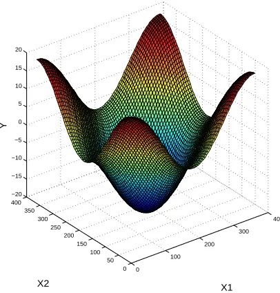
The first example presents a 2-D non-linear function. The output of the function Y is represented by the equation:

Y = 10cos(X1) + 10sin(X2) (14)

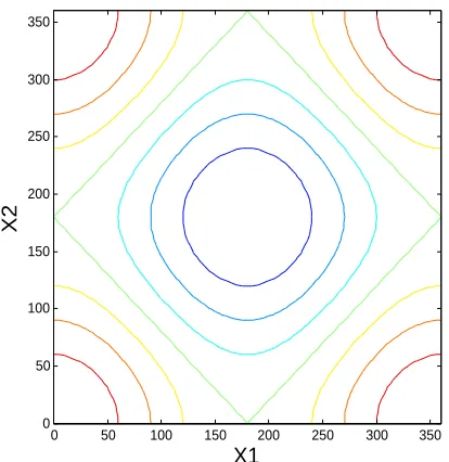
where the model state variablesX1 andX2 are uniformly and independently distributed in the range of 0 and 360 degrees. For this current reliability analysis, the failure criteria (F =g(X)≤0) of the model is defined as when the model outputY exceeds 15. The surface and contour plot of the function is shown in Fig.1 and 2.

0 100 200 300 400 0 50 100 150 200 250 300 350 400 −20 −15 −10 −5 0 5 10 15 20 X1 X2 Y

X1

X2

0 50 100 150 200 250 300 350 0

50 100 150 200 250 300 350

Figure 2: Contour Plot of Safety Function

Given that the proposed will be tested, the objectives of this example will involve training multiple ANNs based on the same architecture, compute the failure probability ˆpF from each of the each of the ANNs based on the failure

criteria (F = g(X)≤ 0) defined, compute the robust estimate of ˆ(pF), and

finally quantify the uncertainty in the the robust estimate of ˆ(pF) due to

model uncertainty.

3.2. Analysis

Training samples Dtrain(x, y) of size N = 100 have been generated via

Latin hypercube sampling (LHS) algorithm[31] from Eq.(14). Two setsZ1 =

Ni, i = 1,2, ...M and Z2 = Ni, i = 1,2, ...M composed of M = 10 identical

ANNs have been trained based on Dtrain(x, y). Specifically, in the first set

(Z1), all the training samples inDtrain(x, y) have been used to train the ANNs

training samples Dtrain have been used to train the ANNs and the remaining

20% used for validation. The network architecture chosen for the ANNs in both sets composed of three hidden layers (2,5,1). Next, the posterior probability of the ANNs in set Z1 has been estimated using Bayes’ formula

given in Eq. (1) by assigning uniform prior probabilityP(Nk) = 1/M to each

ANN. On the other hand, the R2 validation values for the ANNs in set Z2

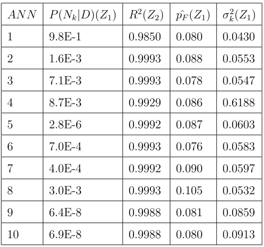
have been estimated based on the validation samples. The results of these analysis are given in Table.1 for robust comparison. It should be noted that

ith _{ANN in both set (Z}

1 andZ2) have been trained inside the same iteration

loop, hence it is assumed that their resultant behaviour should be similar, except that the ANNs in Z1 are expected to have a higher performance

capability due to more training samples used to train them. As shown in Table.1, although the ANNs Ni, i= 1,2, ..M in sets Z1 and Z2 are identical

as they have been trained in the same iteration loop, there is no agreement between the posterior probability estimated from the ANNs in Z1 and the

corresponding R2 validation values estimated from the ANNs in Z2. This

finding is further supported by the fact that the best model selected (N1)

based on its posterior probability has the lowest R2 value. Hence, we can support our claim that the use of R2 _{value to select the best model is a}

biased method. Further, to implement the proposed approach, the ANNs in Z1 have been chosen as they have higher predictive capability (i.e. more

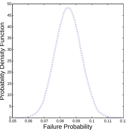
samples used to train them). To accurately compute a robust estimate of ˆ

pF, 104 Monte Carlo simulation runs have been used for each ANN, and the

value. Finally, the model uncertainty propagated to robust prediction of ˆpF

has been quantified in terms of confidence intervals estimated from Eq.(12) and Eq.(13).

Table 1: Simulation Results for Non-linear Function

AN N P(Nk|D)(Z1) R2(Z2) pˆF(Z1) σ2k(Z1)

1 9.8E-1 0.9850 0.080 0.0430

2 1.6E-3 0.9993 0.088 0.0553

3 7.1E-3 0.9993 0.078 0.0547

4 8.7E-3 0.9929 0.086 0.6188

5 2.8E-6 0.9992 0.087 0.0603

6 7.0E-4 0.9993 0.076 0.0583

7 4.0E-4 0.9992 0.090 0.0597

8 3.0E-3 0.9993 0.105 0.0532

9 6.4E-8 0.9988 0.081 0.0859

0.050 0.06 0.07 0.08 0.09 0.1 0.11 0.12 5

10 15 20 25 30 35 40 45 50

Failure Probability

Probability Density Function

Figure 3: Model Uncertainty Propagated to ˆpF Using the Proposed Approach

3.3. Verification of the Proposed Approach for Reliability Analysis

To verify that the true value of ˆpF falls within the robust confidence

interval derived from the approach, the real model given in Eq.(14) has been used to estimate the true value of ˆpF adopting the same failure

cri-teria (i.e. Y > 15). Similarly, 104 Monte Carlo simulation runs have been used to estimate the true value of the failure probability ˆpF = 0.0870. This

value obtained ( ˆpF = 0.0870) verifies that the proposed approach is robust

enough to estimate a prediction that converges to the true value. Finally, to investigate the number of ANNs that must be trained for the predic-tion (i.e. ˆpF) that converges to the true unbiased value, a different number

prediction E(yadj) has been estimated. The results are shown in Fig.(4).

0.065 0.07 0.075 0.08 0.085 0.09 0.095 0.1

1 2 3 4

Failure Probability p

F

M=1000 M=10000 M=100

M=10

Figure 4: Confidence Intervals ofpF for Different Number of Trained ANNs

3.4. Example 2

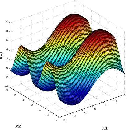
The second example used to test the proposed approach adopts the well known the Ishigami function. This function is often used as a benchmark model to test different sensitivity analysis methods. The function is repre-sented by the following equation:

f(X) =sin(X1) +asin2X2 +bX34sin(X1) (15)

In this example, the numerical values chosen for a and b are 7 and 0.1 re-spectively. The parameters Xi, i = 1,2,3 are uniformly distributed in the interval of −πand π. The surface plot of the non-linear function is shown in Fig.5. −3 −2 −1 0 1 2 3 −3 −2 −1 0 1 2 3 −4 −2 0 2 4 6 8 10 X1 X2 f(X)

Figure 5: Ishighami fuction: Relationship between X1 and X2

3.5. Analysis

Here, training samples Dtrain of size N = 100 have been generated via

Latin hypercube algorithm [31]. Once again, two sets Z1 =Ni, i= 1,2, ...M

and Z2 = Ni, i = 1,2, ...M containing M = 10 ANNs with a three hidden

layer configuration of (3,13,1) have been constructed and used as a substitute for the Ishigami function. In a similar fashion as carried out in the first example, the ANNs in the first set (Z1) have been trained with 100% of

Dtrain(x, y), while 80% Dtrain(x, y) have been used to train the ANNs in the

second set (Z2), and the remaining 20% used to compute the R2 validation

error. Using Bayes’ formula given in Eq. (1) the posterior probability of each ANN in Z1 have been estimated by assuming a uniform prior probability

P(Nk) = 1/M. Tables.2 and 3 shows the summary of the results obtained.

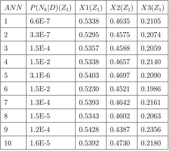
Again, comparing the posterior probability and theR2 validation error shows that there is no correlation between them. For instance, the 9th_{and 10}th_ANN

have the highest R2 values, however, their respective posterior probability are relatively low compared to other ANNs. Hence, selecting them based on theirR2 validation error can result to biased values, when used for prediction. Henceforth, the ANNs in Z1 have been selected to implement the proposed

approach. To compute the robust predicted quantity, Saltelli’s algorithm [32] has been used to estimate Si and Ti for all the ANNs adopting N = 105

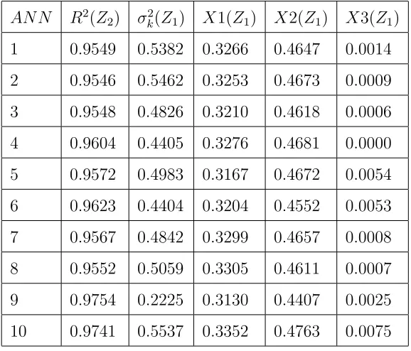
Table 2: Quantities Estimated from Identical ANNs (NB:Xi, i= 1,2,3 is the First Order

Sensitivity Indices Estimated fromZ1)

AN N R2(Z2) σk2(Z1) X1(Z1) X2(Z1) X3(Z1)

1 0.9549 0.5382 0.3266 0.4647 0.0014 2 0.9546 0.5462 0.3253 0.4673 0.0009 3 0.9548 0.4826 0.3210 0.4618 0.0006 4 0.9604 0.4405 0.3276 0.4681 0.0000 5 0.9572 0.4983 0.3167 0.4672 0.0054 6 0.9623 0.4404 0.3204 0.4552 0.0053 7 0.9567 0.4842 0.3299 0.4657 0.0008

Table 3: Quantities Estimated from Identical ANNs (NB:Xi, i= 1,2,3 is the Total Effect

Sensitivity Indices Estimated fromZ1)

AN N P(Nk|D)(Z1) X1(Z1) X2(Z1) X3(Z1)

1 6.6E-7 0.5338 0.4635 0.2105

2 3.3E-7 0.5295 0.4575 0.2074

3 1.5E-4 0.5357 0.4588 0.2059

4 1.5E-2 0.5338 0.4657 0.2140

5 3.1E-6 0.5403 0.4697 0.2090

6 1.5E-2 0.5230 0.4521 0.1986

7 1.3E-4 0.5393 0.4642 0.2161

8 1.5E-5 0.5343 0.4602 0.2063

9 1.2E-4 0.5428 0.4387 0.2356

10 1.6E-5 0.5392 0.4730 0.2180

Table 4: Quantified Uncertainty in Robust Pridiction for First Order Sensitivity Indices

P arameter CI CI V ar(Si) E(Si)

X1 0.3138 0.3347 7.9E-6 0.3139

X2 0.4416 0.4766 18.3E-6 0.4418

Table 5: Quantified Uncertainty in Robust Pridiction for Total Effect Sensitivity Indices

P arameter CI CI V ar(Si) E(Si)

X1 0.5429 0.5462 27E-6 0.5430

X2 0.4388 0.4787 39E-6 0.4389

X3 0.2357 0.2365 40E-6 0.2358

3.6. Verification of Proposed Approach for Sensitivity Analysis

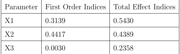
To verify the robust sensitivity indices obtained from the approach con-verges to the true value, a comparison has been made with the predicted value estimated from the real model. Adopting N = 105 _{Monte Carlo}

sam-ples, the real sensitivity indices have been computed directly from the real model with Saltelli’s algorithm [32] (see Table.6) The results show that the robust values obtained from the approach is close to the real value estimated from the real model. Hence, we conclude that our approach is sufficient enough to increase the robustness of the prediction made by ANN.

Table 6: Sensitivity Indices Estimated from the Real Model

Parameter First Order Indices Total Effect Indices

X1 0.3139 0.5430

X2 0.4417 0.4389

4. Case Study

Once again, the applicability of the proposed approach is demostrated by performing reliability and sensitivity analysis on a real case study. This case study focuses on a complex and expensive mathematical model of the Site Ion eXchange Effluent Plant (SIXEP)(see [33]) situated on the nuclear fuel reprocessing and decommissioning site at Sellafield, U.K. Sellafield site is one of the largest nuclear installations in the world and is arguably the most complex nuclear site in the world due to the fact there is a lot of engi-neering and history present in a fairly small area. SIXEP plant is one of two effluent treatment plants that manage discharges of radioactivity across the whole site. This is a highly complex engineered system. The plant works by capturing radioactivity present in a mobile form in the aqueous waste stream into an immobile solid form by a process of filtration and ion exchange. The SIXEP plant was commissioned in the mid 1980’s and immediately resulted in the reduction of radioactivite discharge from the Sellafield site to less than 1% of the prior level. A schematic diagram of the SIXEP is shown in Fig.6.

agency [33].

4.1. Uncertainties Affecting the SIXEP

There is uncertainty of the future feeds composition arising from the Sel-lafield site, leading to variability in the activity levels of Caesium-137 and Strontium-90 and other soluble species that affect the removal of these iso-topes. This variability can cause undesirable consequences to the environ-ment (i.e. the discharges of the two afore-environ-mentioned radionuclides exceeds their desired levels). Therefore, it is nessessary to include this uncertainty into studies when using the SIXEP model to assess the risk associated with the SIXEP model, and identify thoes model parameters that contribute sig-nificantly to this variability. It should be noted that the uncertainty consid-ered to affect the plant feeds are aleatory (i.e. random) in nature [1]. The consideration of this type of uncertainty leads to defining of a state vectorx

of 18 state variables of the SIXEP model x = xn:n= 1,2, ..,18, which are

assumed to be described by the probability distributions given in Table.7. The schematic of the SIXEP model is shown in Fig.7.

𝒙_𝟏

𝒙𝒏 𝒙𝟑 𝒙𝟐

gPROMS

𝒇(𝒙𝒊)

𝒎𝒂𝒙(𝑪𝒔-137)

𝒎𝒂𝒙(𝑺𝒓-90)

Table 7: SIXEP Model Input Parameters

P arameterID M ean S.T.D LowerBound U pperBound

1 0.50E+3 0.66E+3 0.01E+2 6.63E+3

2 39.0E+3 37.0E+3 1.00E+3 210E+3

3 1.05E+3 359E+3 0.11E+3 3.00E+3

4 0.03E+3 0.02E+3 0.01E+4 0.13E+4

5 46.0E-6 36.0E-6 3.00E-6 494E-6

6 6.13E-3 1.83E-3 1.14E-3 1.42E-3

7 1.59E-5 1.28E-5 0.25E-5 14.7E-5

8 9.40E-6 1.05E-5 2.50E-7 1.06E-4

9 15.9E+4 7.10E+4 1.90E-4 4.81E+5

10 0.45E+2 0.49E+2 0.20E+1 0.24E+3

11 2.00E+3 0.62E+3 0.73E+3 4.00E+3

12 0.33E+2 0.39E+2 4.00E-2 5.30E+2

13 0.14E+1 0.30E+1 3.00E-2 0.37E+2

14 3.84E-6 1.22E-5 0.40E-12 1.06E-4

15 3.50E-6 2.82E-4 2.74E-3 4.61E-3

16 3.20E-6 3.28E-6 2.56E-7 3.5E-5

17 2.38E-6 2.93E-6 2.50E-11 2.50E-5

18 2.00E+6 2.79E+5 7.03E+5 3.00E+6

Henceforth, the state variables x =xn :n= 1,2, ..,18 map out two

uncertainties from the state variables via Monte Carlo simulation through the model gives rise to variability in the performance variables. The uncer-tainty propagation has been performed by generating 1000 samples and the maximum concentration of the two radionuclides are shown in the histograms given in Fig.9 and 10. The failure criteria (F =X :g(X)≤0) of the model has been defined as when the performance variables exceeds unity.

0 100 200 300 400 500 600

0 1 2 3 4 5 6x 10

−3

Time in Days

Normalized Activity

Caesium−137 Strontium−90

0 0.5 1 1.5 2 2.5 3 0

50 100 150 200 250 300 350 400

Normalised Maximum Caesium−137

Frequency

Figure 9: Normalized Variability in Maximum Caesium-137

0 0.2 0.4 0.6 0.8 1 1.2 1.4

0 5 10 15 20 25 30 35 40

Normalised Maximum Strontium−90

Frequency

Figure 10: Normalized Variability in Maximum Strontium-90

paper is been adopted to quantify the failure probability, and identify the contributions of the state variables to the variation in the performance vari-able.

4.2. Construction of ANN for Reliability and Sensitivity Analysis

As a single evaluation of the model requires approximately 1200 seconds for running a single process, ANN have been used as a substitute to speed up the time required for reliability and sensitivity analysis. To construct the network, training set Dtrain(x, y) of sample size Ntrain = 1021 have been

obtained by evaluating the model repeatedly. Specifically, the training data set Dtrain(x, y) have been generated via the LHS algorithm, considering the

18 state variables to be uniformly distributed. The idea behind using uniform distributions is to explore the admissible range of variability within each of the state variable. The hyper-parameters of the uniform distributions chosen to represent the state variables are identical to those specified in Table.7. Scalar quantities of the performance variablesy=y1, y2 have been computed,

where y1 and y2 represents the maximum concentration of Caesium-137 and

Strontium-90 respectively. The choice of the ANN architecture is vital for an accurate representation of the SIXEP model. In particular, three hidden layer configuration (18,9,2) have been chosen.

4.3. Training multiple Identical ANN

Here, two sets Z1 =Ni, i= 1,2, ...M and Z2 =Ni, i = 1,2, ...M

contain-ing M = 1000 ANNs have been trained. As done in the previous examples, 100% of the training samples have been used to train all the ANNs in Z1,

and the remaining 20% used for validation. The posterior probability of the ANNs in Z1 has been estimated by assigning uniform prior probability

P(Nk) = 1/M to each ANN. In addition, theR2 validation errors have been

computed for the ANNs in Z2. For brevity, a summary of the top and

bot-tom 5 ANNs based on their posterior probability and variance are shown in Tables 8-11. The same tables also show the R2 validation error for a robust comparison.

Table 8: Top 5 ANN for Max Caesium-137

AN N σ2_k(Z1)) P(Dtrain|Nk)(Z1) R2(Z2)

1 0.18E-6 0.162 0.9623

2 0.19E-6 0.116 0.9498

3 0.20E-6 0.107 0.9586

4 0.21E-6 0.058 0.9465

Table 9: Bottom 5 ANN for Max Caesium-137

AN N σ2

k(Z1) P(Dtrain|Nk)(Z1) R2(Z2)

1 1.62E-2 0.0029 0.8839

2 1.67E-2 0.0047 0.8880

3 1.72E-2 0.0087 0.8990

4 1.77E-2 0.0066 0.6205

5 1.83E-2 0.0012 0.6140

Table 10: Top 5 ANN for Max Strontium-90

AN N σ2

k(Z1) P(Dtrain|Nk)(Z1) R2(Z2)

1 1.62E-6 0.165 0.9275

2 1.18E-6 0.122 0.9330

3 1.10E-6 0.087 0.9594

4 1.06E-6 0.066 0.9588

Table 11: Bottom 5 ANN for Max Strontium-90

AN N σ2

k(Z1) P(Dtrain|Nk)(Z1) R2(Z2)

1 1.20E-2 0.0016 0.8892

2 1.18E-2 0.0012 0.7948

3 1.10E-2 0.0008 0.8993

4 1.06E-2 0.0066 0.8969

5 1.04E-2 0.0047 0.8918

Again, as shown in Tables 8-11, there is no correlation between the R2

validation error and the posterior probability computed for each ANN (i.e. a highR2 does not indicate the best model). For example, in Table. 8 when comparing the 4th _{and 5}th _{ANNs, the R}2 _{value of the 5}th _{is 0.9588 which is}

greater than the R2 value of the 4th ANN (0.9456). However, the posterior probability of the 4th_{ANN is greater than the posterior probability of the 5}th

ANN. This confirms that a high R2 validation error does not mean a better model.

4.4. Robust Estimate of Failure Probability

In this section, the ANNs in Z1 have been adopted to implement the

proposed approach in order to compute a robust estimate of the failure probability. Specifically, 104 samples have been used to compute the fail-ure probability ˆpF in each ANN. To reduce the computational time for this

to compute the robust estimate of ˆpF. Finally, confidence intervals of robust

estimate quantifying the model uncertainties has been estimated based on Eqs. (12) and (13), and the result is shown in Fig.11.

0 1 2 3 4 5 6 7 8

x 10−4

1

Failure Probability

Figure 11: Confidence Intervals in Robust Prediction of the Probability of Failure

Although the confidence interval shown in Fig.11 is fairly wide, the most probable estimate of the true failure probability is represented by the mean of the interval(i.e. shown in red).

4.5. Robust Estimate of Sensitivity Indices

In this section, the ANNs in Z1 have been adopted to implement the

estimate of Si and Ti. Finally, the model uncertainty propagated to the

ro-bust estimates have been quantified in terms of confidence intervals (see Figs. 12-15).

0 0.2 0.4 0.6 0.8 1

1 2 3 4 5 6 7 8 9 10 11 12 13 14 15 16 17 18 Uncertain Parameter ID

First Order Sensitivity Measures

Figure 12: Confidence Intervals in Robust Prediction of First Order Sensitivity Indices

0 0.2 0.4 0.6 0.8 1 1.2

1 2 3 4 5 6 7 8 9 10 11 12 13 14 15 16 17 18 Uncertain Parameter ID

Total Effect Sensitivity Measure

Figure 13: Confidence Intervals in Robust Prediction of Total Effect Sensitivity Indices

(contributions to Cs-137)

−0.2 0 0.2 0.4 0.6 0.8 1 1.2 1.4

1 2 3 4 5 6 7 8 9 10 11 12 13 14 15 16 17 18 Uncertain Parameter ID

First Order Sensitivity Measure

Figure 14: Confidence Intervals in Robust Prediction of First Order Sensitivity Indices

−0.2 0 0.2 0.4 0.6 0.8 1 1.2 1.4

1 2 3 4 5 6 7 8 9 10 11 12 13 14 15 16 17 18 Uncertain Parameter ID

Total Effect Sensitivity Measure

Figure 15: Confidence Intervals in Robust Prediction of Total Effect Sensitivity Indices

(contributions to Sr-90)

From the results shown in Figs. 12-15, the state variables that have higher contributions (i.e. 7th parameter) tend to have larger confidence intervals. A possible reason for these large intervals may be that the performance of an ANN reduces when estimating significant variables as a result of noise and other factors not known to the authors. However, the expected value (i.e. shown in red) is the most likely estimate that is to be taken as the true value when adopting the proposed approach.

5. Conclusions

for an expensive model to speed up the time required for the aforementioned analysis. However, the use of ANN for these kind of analysis introduces additional uncertainties into the predicted quantity. Therefore, it is vital to quantify the uncertainties in order to ensure a robust prediction. On the other hand, training a unique ANN architecture repeatedly results to variability in terms of their performance. This variability is as a result of the error function within each ANN being trapped in a different local minima. Hence, an additional uncertainty is introduced due to the lack of knowledge about the best performing ANN. Consequently, the use of cross-validation technique (i.e. k−f old) to evaluate the performances of these ANNs based on theirR2

value is not an adequate measure due to the possibility to having a low R2

value for a good ANN, and a high R2 value for an ANN that does not fit the model adequately. In addition, the use of only part of the data set to train the ANN is wasteful of information, and drastically decreases accuracy in estimating the weight parameters of the ANN. Hence, we postulate that the use of cross-validation technique to select the best ANN out of a set of ANN with identical architecture introduces biassing and reduces the robustness of the predicted quantity.

from this study shows that the true value of the quantity to be predicted by the ANN is close to the expected value given from our proposed approach, and within the confidence bounds that quantifies the model uncertainty. This model uncertainty quantification is of paramount importance in safety criti-cal applications, in particular when few data representative are used to train an Artificial Neural Network.

Acknowledgements

This work has been partially supported by the EPSRC Grant EP/M018717/1 (Smart on-line monitoring for nuclear power plants (SMART)) and by the IRSES Marie Curie action of the European Union FP7-PEOPLE-2013-IRSES (Large Multipurpose Platforms for Exploiting Renewable Energy in Open Seas (PLENOSE)).

[1] J. C. Helton, D. E. Burmaster, Guest editorial: treatment of aleatory and epistemic uncertainty in performance assessments for complex sys-tems, Reliability Engineering & System Safety 54 (2) (1996) 91–94.

[2] E. Patelli, D. A. Alvarez, M. Broggi, M. de Angelis, Uncer-tainty management in multidisciplinary design of critical safety sys-tems, Journal of Aerospace Information Systems 12 (2015) 140–169. doi:10.2514/1.I010273.

[3] P. Bjerager, On computation methods for structural reliability analysis, Structural Safety 9 (2) (1990) 79–96.

[5] R. Melchers, Importance sampling in structural systems, Structural safety 6 (1) (1989) 3–10.

[6] O. Ditlevsen, P. Bjerager, R. Olesen, A. Hasofer, Directional simulation in gaussian processes, Probabilistic Engineering Mechanics 3 (4) (1988) 207–217.

[7] P. Koutsourelakis, H. Pradlwarter, G. Schu¨eller, Reliability of structures in high dimensions, part i: algorithms and applications, Probabilistic Engineering Mechanics 19 (4) (2004) 409–417.

[8] M. de Angelis, E. Patelli, M. Beer, Advanced line sampling for efficient robust reliability analysis, Structural Safety 52 (2015) 170–182.

[9] S.-K. Au, J. L. Beck, Estimation of small failure probabilities in high dimensions by subset simulation, Probabilistic Engineering Mechanics 16 (4) (2001) 263–277.

[10] S.-K. Au, E. Patelli, Rare event simulation in finite-infinite dimensional space, Reliability Engineering & System Safety 148 (2016) 67–77.

[11] A. Saltelli, K. Chan, E. M. Scott, et al., Sensitivity analysis, Vol. 1, Wiley New York, 2000.

[12] T. Homma, A. Saltelli, Importance measures in global sensitivity analy-sis of nonlinear models, Reliability Engineering & System Safety 52 (1) (1996) 1–17.

un-certainty management of large finite element models, Finite elements in analysis and design 51 (2012) 31–48.

[14] E. Patelli, COSSAN: A Multidisciplinary Software Suite for Uncertainty Quantification and Risk Management, Springer International Publish-ing, Cham, 2016, pp. 1–69.

[15] G. Baroni, S. Tarantola, A general probabilistic framework for uncer-tainty and global sensitivity analysis of deterministic models: A hy-drological case study, Environmental Modelling & Software 51 (2014) 26–34.

[16] C. M. Bishop, Neural networks for pattern recognition, Oxford univer-sity press, 1995.

[17] J. Cheng, Q. Li, R.-c. Xiao, A new artificial neural network-based re-sponse surface method for structural reliability analysis, Probabilistic Engineering Mechanics 23 (1) (2008) 51–63.

[18] N. Pedroni, E. Zio, G. E. Apostolakis, Comparison of bootstrapped arti-ficial neural networks and quadratic response surfaces for the estimation of the functional failure probability of a thermal–hydraulic passive sys-tem, Reliability Engineering & System Safety 95 (4) (2010) 386–395.

[19] P. Secchi, E. Zio, F. Di Maio, Quantifying uncertainties in the estimation of safety parameters by using bootstrapped artificial neural networks, Annals of Nuclear Energy 35 (12) (2008) 2338–2350.

temperature in an rmbk-1500 nuclear reactor accident, Nuclear Engi-neering and Design 238 (9) (2008) 2165–2172.

[21] D. E. Rumelhart, G. E. Hinton, R. J. Williams, Learning internal rep-resentations by error propagation, Tech. rep., DTIC Document (1985).

[22] T. Nilsen, T. Aven, Models and model uncertainty in the context of risk analysis, Reliability Engineering & System Safety 79 (3) (2003) 309–317.

[23] G. B. Kingston, H. R. Maier, M. F. Lambert, Bayesian model selection applied to artificial neural networks used for water resources modeling, Water Resources Research 44 (4).

[24] L. Wasserman, Bayesian model selection and model averaging, Journal of mathematical psychology 44 (1) (2000) 92–107.

[25] E. Zio, A study of the bootstrap method for estimating the accuracy of artificial neural networks in predicting nuclear transient processes, IEEE Transactions on Nuclear Science 53 (3) (2006) 1460–1478.

[26] M. Bayarri, J. Berger, J. Cafeo, G. Garcia-Donato, F. Liu, J. Palomo, R. Parthasarathy, R. Paulo, J. Sacks, D. Walsh, Computer model valida-tion with funcvalida-tional output, The Annals of Statistics (2007) 1874–1906.

[27] M. J. Bayarri, J. O. Berger, R. Paulo, J. Sacks, J. A. Cafeo, J. Cavendish, C.-H. Lin, J. Tu, A framework for validation of computer models, Tech-nometrics.

Journal of the Royal Statistical Society: Series B (Statistical Methodol-ogy) 63 (3) (2001) 425–464.

[29] D. G. Kleinbaum, M. Klein, Maximum likelihood techniques: An overview, in: Logistic regression, Springer, 2010, pp. 103–127.

[30] T. H. Wonnacott, R. J. Wonnacott, Introductory statistics, Vol. 19690, Wiley New York, 1972.

[31] J. C. Helton, F. J. Davis, Latin hypercube sampling and the propagation of uncertainty in analyses of complex systems, Reliability Engineering & System Safety 81 (1) (2003) 23–69.

[32] A. Saltelli, Making best use of model evaluations to compute sensitivity indices, Computer Physics Communications 145 (2) (2002) 280–297.

[33] S. Owens, M. Higgins-Bos, M. Bankhead, J. Austin, Using chemical and process modelling to design, understand and improve an efluent treatment plant., NNL Science, 3, (2015) 4–13.