City, University of London Institutional Repository
Citation
:
Li, A., Broom, M., Du, J. & Wang, L. (2016). Evolutionary dynamics of general group interactions in structured populations. Physical Review E (PRE), 93(2), 022407. doi: 10.1103/PhysRevE.93.022407This is the accepted version of the paper.
This version of the publication may differ from the final published
version.
Permanent repository link:
http://openaccess.city.ac.uk/13883/Link to published version
:
http://dx.doi.org/10.1103/PhysRevE.93.022407Copyright and reuse:
City Research Online aims to make research
outputs of City, University of London available to a wider audience.
Copyright and Moral Rights remain with the author(s) and/or copyright
holders. URLs from City Research Online may be freely distributed and
linked to.
City Research Online: http://openaccess.city.ac.uk/ [email protected]
Evolutionary dynamics of general
group interactions in structured populations
Aming Li1,2, Mark Broom3, Jinming Du1, and Long Wang1,∗
1. Center for Systems and Control, College of Engineering, Peking University, Beijing
100871, China
2. Center for Complex Network Research and Department of Physics, Northeastern
Uni-versity, Boston, Massachusetts 02115, USA
3. Department of Mathematics, City University London, Northampton Square, London
EC1V 0HB, UK
(Dated: February 5, 2016)
Abstract
The evolution of populations is influenced by many factors, and the simple classical models
have been developed in a number of important ways. Both population structure and multi-player
interactions have been shown to significantly affect the evolution of important properties, such
as the level of cooperation or of aggressive behavior. Here we combine these two key factors
and develop the evolutionary dynamics of general group interactions in structured populations
represented by regular graphs. The traditional linear and threshold public goods games are adopted
as models to address the dynamics. We show that for linear group interactions, population structure
can favor the evolution of cooperation compared to the well-mixed case, and see that the more
neighbors there are, the harder it is for cooperators to persist in structured populations. We further
show that threshold group interactions could lead to the emergence of cooperation even in
well-mixed populations. Here population structure sometimes inhibits cooperation for the threshold
public goods game, where depending on the benefit to cost ratio, the outcomes are bi-stability or
a monomorphic population of defectors or cooperators. Our results suggest, counter-intuitively,
that structured populations are not always beneficial for the evolution of cooperation for nonlinear
group interactions.
I. INTRODUCTION
The evolution of cooperation is an enduring conundrum in evolutionary biology since Darwin [1–7]. Serving as an indispensable mathematical model, evolutionary game theory [5, 6, 8–10] has become an effective method to quantify cooperation and predict evolutionary outcomes for different situations. Some further theoretical analyses on the evolution of cooperation have been achieved since the introduction of evolutionary dynamics in both infinite and finite populations [4, 6, 11–13]. Within the area of dynamics, two-player games [14–16] are frequently adopted to model typical pairwise interactions to understand the evolution of cooperation [17–26]. Considering the ubiquitously group interactions ranging from the natural world to human society, researchers recently generalized two-player games to their multi-player versions [27–37], such as the N-person prisoner’s dilemma [30, 38], N-person snowdrift game [31, 32], N-person stag hunt game [39], as well as the N-person ultimatum game [40]. In a typical collective action, an individual’s payoff could be no longer the simple summation of many pairwise interactions [33, 41], and instead it is replaced by the multiple interactive payoffs from multi-player games, which depends on what strategies all other opponents hold in the same group. The various compositions of different strategies in group interactions give the possibility for the emergence of nonlinear fitness [29].
Spatial reciprocity is generally accepted as one of the five rules facilitating the evolution of cooperation [7], and some theoretical results as well as experiments have validated this rule by illustrating the positive function of spatial interactions represented by lattice or com-plex networks [17, 33, 46, 49–52]. However, we should not ignore some special cases where the detrimental effect of spatial structure on cooperation is revealed under the framework of the snowdrift game [18]. The presence of both multi-player games and population structure enriches the outcomes of evolutionary dynamics. Moreover, as we consider general group interactions in structured populations, we are provided with a much greater chance to ex-plore the effects of population structure on the evolution of cooperation. However, due to its inherent complexity, until now the evolutionary dynamics has only been given for some specific games or well-mixed populations [12, 31, 32, 39, 44, 45, 48, 53, 54]. Here we give the evolutionary dynamics for an arbitrary multi-player game with two strategies in struc-tured populations represented by regular graphs. Whatever the specific form of the payoff functions, the general multi-player game just requires the discrete payoff values on every possible composition of strategies. Moreover, two typical multi-player games are employed as examples to explore the evolution of cooperation in structured populations. We find that some counter-intuitive results are obtained from these examples.
II. MODEL
(b)
(a) (c) (d)
a3 a2 a2
[image:6.612.84.531.72.193.2]a3
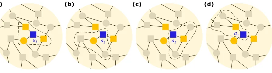
FIG. 1: Group interactions in structured populations. We choose 14 individuals from a population
with degree k = 3 to explain group interactions in structured populations. The nodes shown as squares and circles represent individuals with strategy X and Y, respectively. The individual with a blue square has three neighbors (colored orange). During evolution, in each generation,
every player will organize a game with a group of size k+ 1 comprising itself and its neighbors. Taking the blue square as an example, we find that its payoff consists of four games: one organized
by itself (circled by the dashed line in (a)), and another three organized by its three neighbors
independently (circled by the dashed line in (b), (c), and (d)). Using the payoff matrix, we give
the corresponding payoff of the blue square in each panel, where the subscript indicates the number
of individuals involved in the game with strategyX. Payoffs of other individuals can be calculated in the same way in each generation, and after that, a death-birth process is employed to characterize
the evolution of strategies in the population.
for a general multi-player game with size n=k+ 1 is presented as OpposingX players 0 1 · · · i · · · k−1 k
X a0 a1 · · · ai · · · ak−1 ak
Y b0 b1 · · · bi · · · bk−1 bk
where ai and bi depict the payoffs obtained by the players with strategy X and Y,
respec-tively. The subscriptiis the number of players adopting strategyXin the game (see Fig. 1). Based on the payoffs of each individual, the “death-birth” (DB) process is employed to cap-ture the update process, where an individual in the population is randomly chosen to die at each evolutionary step, and then all of its neighbors compete for the vacant site, gaining it with probability proportional to their fitness.
[19, 46, 55, 56]. The notations, pXY and pX are used to indicate the frequency of XY
pairs and strategy X. For an individual with strategy Y, the probability for him or her to find someone with strategy X is qX|Y. Hence based on the above definitions, we have the
relations between these notations as
pX +pY = 1
qX|X +qY|X = 1
pXY =pY ·qX|Y
pXY =pY X
where in this physical system, all variables could be represented by pX and qX|X.
After long calculations with the evolutionary process of the whole population captured bypX andqX|X, we find that the global frequency change ofpX is very slow due to the weak
selection intensity w [19, 46, 56]. Furthermore, we have
qX|X =
k−2 k−1pX +
1
k−1 (1)
at evolutionary equilibrium based on the separation of two time scales [57]. According to the above relation between pX and qX|X, all variables in the dynamic evolutionary system can
be expressed only by pX mathematically when it is stable (for the detailed deviations, see
[46]). It elucidates that as the composition of the structured population in term of individual strategies is stable, we could obtain the more detailed information about the population by considering only the fraction of the players with strategy X.
Hence, as we use x to indicate the expected change of the frequency of cooperators, we have the deterministic evolutionary dynamics
˙
x= w(k−2)
k(k−1)x(1−x)f(x) (2)
where f(x) = k(πY
X −πYY) + [(k−2)x+ 1]
(πX
X −πYX)−(πYX −πYY)
, and πY
X is the mean
structure around the selected individual who haskX neighbors adopting strategyX, we have
πXX =akX +
k−1
X
i=0 p(i)∗
"
ai+1+i
k−1
X
l=0
p(l)al+1+ (k−1−i)
k−1
X
l=0 q(l)al
#
,
πXY =bkX+1+
k−1
X
i=0 q(i)∗
"
bi+1+i
k−1
X
l=0
p(l)bl+1+ (k−1−i)
k−1
X
l=0 q(l)bl
#
,
πXY =akX−1+
k−1
X
i=0 p(i)∗
"
ai+i k−1
X
l=0
p(l)al+1+ (k−1−i)
k−1
X
l=0 q(l)al
#
,
πYY =bkX +
k−1
X
i=0 q(i)∗
"
bi+i k−1
X
l=0
p(l)bl+1+ (k−1−i)
k−1
X
l=0 q(l)bl
#
.
p(i) andq(i) are the function of i,
p(i) = (k−1)! i!(k−1−i)!q
i X|Xq
k−1−i Y|X ,
q(i) = (k−1)! i!(k−1−i)!q
i X|Yq
k−1−i Y|Y ,
which denote the probability for players (who are neighbors of the selected individual) adopting strategy X and Y to find i players with strategy X and k −1 −i with Y in the player’s other k−1 neighbors except the selected individual, respectively, where qX|X =
(k−2)x/(k−1)+1/(k−1), qX|Y = (k−2)x/(k−1), qY|X = (k−2)(1−x)/(k−1), andqY|Y =
1−(k−2)x/(k−1).
III. LINEAR PUBLIC GOODS GAME
For the traditional public goods game [30], every cooperator contributes a benefitb to the group at a cost c (b > c), while defectors pay nothing, and eventually the totally collected benefits from all cooperators are distributed evenly to every group member irrespective of their previous strategies. As to the payoff matrix, mapping X and Y to the strategy cooperation and defection severally, we have
ai =
(i+ 1)b n −c,
bi =
ib n,
with 0≤i≤n−1, and the corresponding evolutionary dynamics for well-mixed populations is
˙
where n is the group size. According to equation (2), we obtain the evolutionary dynamics (see Appendix A)
˙
x = w(n−3)
n−2 x(1−x)
n+ 2 n b−nc
(4)
in structured populations where every individual has k neighbors (n =k+ 1 here). Consid-ering n > n2/(n+ 2), the evolutionary dynamics indicates that the structured populations could better pave the way for cooperation than the structureless cases (see Fig. 2a, 2b, 2d, and 2e). It has also been pointed out that the benefit and cost of the cooperative behavior only experience a linear payoff transformation as we move from the structureless population to the structured [48]. Now let us consider the net benefit ¯band cost ¯cfor a cooperator. We have the relations
¯
c=c− b
n, ¯b = n−1
n b
between b and ¯b, c and ¯c. Hence we get that cooperation could flourish in a structured population if
¯ b ¯ c >
n(n−1)
2 . (5)
This means that the system will always end up in full cooperation if the above condition is satisfied. As we have shown that, for the structured population represented by the regular graph with degree k, every player has k neighbors and is engaged in group interactions with size n = k+ 1. Our results for group interactions captured by the public goods game in structured populations suggest that cooperators will gain a foothold if the net benefit and net cost ratio ¯b/c¯exceeds half of the product of the number of neighbors and the size of the group interactions.
IV. THRESHOLD PUBLIC GOODS GAME
0 0.5 1 -0.25
0 0.25 0.5
0 0.5 1
10-3 -12 -8 -4 0 4
0 0.5 1
-0.01 0 0.01 0.02
0 0.5 1
-2 0 2 4 6
0 0.5 1
-0.09 -0.06 -0.03 0 0.03
0 0.5 1
-0.050 0.1 0.2
0 0.5 1
10-4 -15 -10 -5 0 5
0 0.5 1
10-3 -5 0 5 10 15 x F ( x ) x x F ( x ) F ( x ) F ( x )
x x x x x
Linear Public Goods Game Threshold Public Goods Game
b/c b/c
b/c b/c
1
1 1
1
n2/(n+2)
n
(n-1)/(n-2) (n-1)(n-2)n-2
W
ell-mi
xed
Structured
x x x
(a) (b) (c)
) e ( )
d
( (f) (g) (h)
0 0.3 -0.10 0.3 xw*
[image:10.612.76.540.69.236.2]xs*
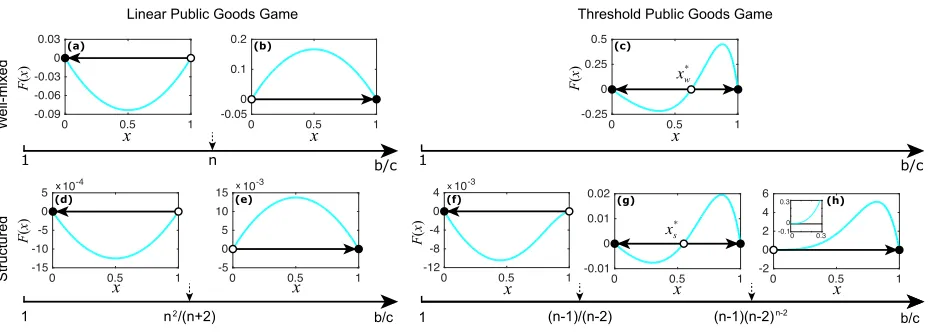
FIG. 2: Evolutionary dynamics for linear and threshold public goods games in well-mixed and
structured populations. Each arrow below the panels gives the range of benefit-to-cost ratiob/c, up to which the corresponding evolutionary dynamics are shown. The direction of selection dynamics
is indicated by the arrow in each panel, where the small solid circle represents a stable equilibrium
while an empty circle represents an unstable equilibrium. In structured populations, the group size
is n = k+ 1. In (c), the internal unstable equilibrium is xw∗, while for (g), it is x∗s. In (h), the inset is employed to show thatF(x)>0 asx→0, and it shares the same labels as the main panel. Parameters are w = 0.01, c = 1, k = 5, n = 6, and the others for (a) and (d) are: b = 4, (b),(c), (e), and (g): b= 10, (f): b= 1.1, (h): b= 2000.
nothing while cooperators still suffer the cost they have paid. In this case, we have ai =
i+ 1
n bθ(i−M + 1)−c, bi =
i
nbθ(i−M)
(6)
where M is the threshold for the collective target, and the Heaviside step function θ(x) satisfies θ(x < 0) = 0 and θ(x≥ 0) = 1. As M = 0 or 1, the threshold public goods game degenerates to its linear version. Here, for simplicity, we consider the largest threshold, M =n.
For the replicator dynamics in well-mixed populations [6], we have
˙
x=x(1−x)(bxn−1−c)
possibility for cooperators to take over the whole population (see Fig. 2c) whatever the value of b/c, i.e. if the initial frequency of cooperators is bigger than x∗w = n−p1
c/b, cooperators will occupy the whole population. However for the linear public goods game, it is impossible for cooperators to take over the population as b/c < n.
When we consider the population structure, according to the equation (2), the evolution-ary dynamics (see Appendix B) is
˙
x= w(n−3)
(n−1)(n−2)x(1−x)
bn[(n−3)x+ 1]
n−1
(n−2)n−2 −n(n−1)c
. (7)
Hence we have that cooperators could take over the population (see Appendix B) if and only if
b c >
n−1
n−2. (8)
For defectors, the criterion is b
c >(n−1)(n−2)
n−2
. (9)
The evolutionary outcomes are divided into three cases based on the value ofb/c(see Fig. 2f to 2h), where pure defectors, bi-stability of defectors and cooperators, and pure cooperators are presented. It shows that a structured population could favor the evolution of cooperation more than a well-mixed population whenb/c >(n−1)(n−2)n−2 (see Fig. 2h), given that in the former case the population will merely consist of cooperators. Whenb/cdecreases but is bigger than (n−1)/(n−2), the advantage of cooperators declines, where, similarly to the well-mixed cases, an internal unstable equilibrium x∗s = (n−p1
(n−1)(n−2)n−2c/b−1)/(n−3) emerges (see Fig. 2g). However we should not miss the situation with b/c <(n−1)/(n−2) where cooperators become extinct (see Fig. 2f), which will never happen for well-mixed populations accompanied by the cooperative attraction interval (n−p1 (n−2)/(n−1),1] (see Fig. 2c), telling us that population structure is not always beneficial for cooperators.
V. DISCUSSION AND CONCLUSIONS
evo-regular graphs, where the payoff functions are not necessarily continuous. Two popular examples, linear and threshold public goods games, are adopted to illustrate the dynamics. We find that the threshold public goods game could give the possibility of the emergence of cooperation with the maximum threshold even when the benefit to cost ratiob/cis small in well-mixed populations, which is impossible for the linear case. Counter-intuitively, we find that population structure is not always helpful for the evolution of cooperation under simple nonlinear group interactions (for example the public goods game with maximum threshold). Our results give another case demonstrating that spatial reciprocity sometimes cannot fa-cilitate the evolution of cooperation under nonlinear group interactions, in addition to the sole preceding one under the metaphor of the snowdrift game [18].
As we explore the effects of population structure on the evolution of cooperation for group interactions, the concept of total payoffs [46, 50] is adopted to capture the interactions, where each individual acquires payoffs from the game organized by itself as well as its neighbors. However for well-mixed populations, the average payoff for each individual is usually considered, i.e., it is the average payoff from one group interaction for individuals with different strategies. We have retained these conventions, since they do not affect our substantive results; if we had used the total payoff for our well-mixed populations, for example, the rate of change in the replicator dynamics would be increased, but the phase space and equilibria would be completely unchanged.
From the perspective of theory, we could consider an example like this: assuming there are k + 1 cooperators (strategy X) in a structured population with the configuration of a cooperator surrounded by k cooperator neighbors, then we have qX|X = 2/(k + 1) and
pX = (k−3)/[(k+ 1)(k−2)] for the structured population according to equation (1). For
the well-mixed case, qX|X = pX, and qX|X could be smaller than that for its structured
counterpart, however, it is possible for well-mixed populations to have more cooperators than structured ones when (k−3)/[(k + 1)(k −2)] < pX < 2/(k+ 1). Thus it is
possi-ble for well-mixed populations sometimes to be better for cooperation (X) than structured populations. We note that the same relationship as equation (1) also occurs for pairwise interactions [19] as well as group interactions with synergy and discounting [46], and it shows that, in probability, population structure could favor the evolution of cooperation [17].
Furthermore, the coevolution of population structure and strategy is explored analytically using linking dynamics, where the evolutionary dynamics derived from well-mixed popula-tions [12] could give good approximapopula-tions for that [22]. For general group interacpopula-tions, it is worth exploring the validation of general evolutionary dynamics on situations where the population structure (not well-mixed) is allowed to switch during evolution (also known as coevolutionary dynamics [58]). Here our result may provide a theoretical approximation for more complicated evolutionary scenarios with the evolution of enormous configurations of population structures.
Acknowledgements
Appendix A: The derivation process of evolutionary dynamics for the public goods
game
For the public goods game, using X and Y to represent cooperation (shorted by C) and defection (shorted byD), we have
k−1
X
i=0
p(i)ai = k−1
X
i=0
(k−1)! i!(k−1−i)!q
i C|Cq
k−1−i D|C
(i+ 1)b k+ 1 −c
= −c+ b k+ 1
"
1 +
k−1
X
i=1
(k−1)!
(i−1)!(k−1−i)!q
i C|Cq
k−1−i D|C
#
= −c+ b k+ 1
1 + (k−1)qC|C
,
k−1
X
l=0
p(l)al+1 =
k−1
X
l=0
(k−1)! l!(k−1−l)!q
l C|Cq
k−1−l D|C
(l+ 2)b k+ 1 −c
= −c+ b k+ 1
2 + (k−1)qC|C
,
k−1
X
l=0
q(l)al = k−1
X
l=0
(k−1)! l!(k−1−l)!q
l C|Dq
k−1−l D|D
(l+ 1)b k+ 1 −c
= −c+ b k+ 1
1 + (k−1)qC|D
,
k−1
X
i=0
q(i)bi = k−1
X
i=0
(k−1)! i!(k−1−i)!q
i C|Dq
k−1−i D|D
ib k+ 1
= b
k+ 1(k−1)qC|D =
k−1
X
l=0 q(l)bl
and
k−1
X
l=0
p(l)bl+1 =
k−1
X
l=0
(k−1)! l!(k−1−l)!q
l C|Dq
k−1−l D|D
(l+ 1)b k+ 1
= b
k+ 1
1 + (k−1)qC|C
Hence we obtain
πDC −πDD = akC−1−bkC +
k−1
X
i=0
p(i)ai− k−1
X
i=0 q(i)bi
+
k−1
X
i=0 p(i)∗
"
i
k−1
X
l=0
p(l)al+1+ (k−1−i)
k−1
X
l=0 q(l)al
#
− k−1
X
i=0 q(i)∗
"
i
k−1
X
l=0
p(l)bl+1+ (k−1−i)
k−1
X
l=0 q(l)bl
#
= −c−c+ b k+ 1
1 + (k−1)qC|C
− b
k+ 1(k−1)qC|D +
k−1
X
i=0 p(i)∗
i∗
−c+ b
k+ 1
2 + (k−1)qC|C
+(k−1−i)
−c+ b
k+ 1
1 + (k−1)qC|D
− k−1
X
i=0 q(i)∗
i∗ b
k+ 1
1 + (k−1)qC|C
+ (k−1−i) b
k+ 1(k−1)qC|D
= −2c+ b k+ 1
1 + (k−1)(qC|C −qC|D)
+
k−1
X
i=0 p(i)∗
−(k−1)c+ b
k+ 1
2i+k−1 + (k2 −3k+ 2)pC
− k−1
X
i=0
q(i) b k+ 1
2i+ (k2−3k+ 2)pC
= −2c+ 2b
k+ 1 −(k−1)c+ b
k+ 1(k−1) + 2b k+ 1
k−1
X
i=0
i(p(i)−q(i))
= −(k+ 1)c+b+ 2b k+ 1 = (k+ 3)b
k+ 1 −(k+ 1)c (A1)
and
πCC −πDC−(πCD−πDD) = akC −bkC+1−(akC−1−bkC)
+
k−1
X
i=0
p(i)(ai+1−ai) + k−1
X
i=0
q(i)(bi−bi+1)
= b
k+ 1
k−1
X
i=0
(p(i)−q(i))
Therefore, substituting equations (A1) and (A2) into equation (2), we get the evolutionary dynamics (4) for the public goods game.
Appendix B: The derivation process of evolutionary dynamics for the threshold
public goods game
For the threshold public goods game shown in equation (6) with M =k+ 1, we have (πCC −πCD)−(πDC −πDD) = p(k−1)(ak−ak−1)
= b
k−2 k−1x+
1 k−1
k−1
and
πCD−πDD = −c− k−1
X
i=0
p(i)c+
k−1
X
i=0 p(i)
"
i
k−1
X
l=0
p(l) (−c) +i p(k−1)b+ (k−1−i)
k−1
X
l=0
q(l) (−c)
#
= b(k−1)
k−2 k−1x+
1 k−1
k
−(k+ 1)c.
Hence we obtain the evolutionary dynamics (7) for the threshold public goods game with n=k+ 1.
Denoting ˙x=F(x), we have F(0) =F(1) = 0, and F0(x) = w(k−2)
k(k−1) [(1−x)f(x)−x f(x) +x(1−x)f
0
(x)].
If F0(1) <0, it means that x= 1 is stable, and we have F0(1)<0⇐⇒f(1) >0⇐⇒ b
c > k k−1. If F0(0) >0, it means that x= 0 is unstable, and we have
F0(0)>0⇐⇒f(0)>0⇐⇒ b
c > k(k−1)
k−1 .
Thus the criteria (8) and (9) are obtained for n =k+ 1.
[1] C. Darwin, On the origin of species (John Murray, London, 1859).
[2] J. von Neumann and O. Morgenstern, Theory of Games and Economic Behavior (Princeton
[3] W. D. Hamilton, Am. Nat.97, 354 (1963).
[4] P. D. Taylor and L. B. Jonker, Math. Biosci. 40, 145 (1978).
[5] J. Smith,Evolution and the Theory of Games(Cambridge University Press, Cambridge, 1982).
[6] J. Hofbauer and K. Sigmund, Evolutionary Games and Population Dynamics (Cambridge
University Press, Cambridge, 1998).
[7] M. A. Nowak, Science314, 1560 (2006).
[8] J. M. Smith and G. R. Price, Nature246, 15 (1973).
[9] M. A. Nowak and K. Sigmund, Science303, 793 (2004).
[10] M. Broom and J. Rycht´aˇr, J. Theor. Bio. 302, 70 (2012).
[11] M. A. Nowak, A. Sasaki, C. Taylor, and D. Fudenberg, Nature428, 646 (2004).
[12] A. Traulsen, J. C. Claussen, and C. Hauert, Phys. Rev. Lett. 95, 238701 (2005).
[13] A. Traulsen, M. A. Nowak, and J. M. Pacheco, Phys. Rev. E 74, 011909 (2006).
[14] A. Rapoport and A. Chammah, Prisoner’s Dilemma: A Study in Conflict and Cooperation,
Ann Arbor paperbacks (University of Michigan Press, Ann Arbor, 1965).
[15] R. Sugden, The Economics of Rights, Co-operation and Welfare (Blackwell, Oxford, New
York, 1986).
[16] B. Skyrms,The Stag Hunt and the Evolution of Social Structure (Cambridge University Press,
Cambridge, 2004).
[17] M. A. Nowak and R. May, Nature359, 826 (1992).
[18] C. Hauert and M. Doebeli, Nature428, 643 (2004).
[19] H. Ohtsuki, C. Hauert, E. Lieberman, and M. A. Nowak, Nature441, 502 (2006).
[20] F. Fu, C. Hauert, M. A. Nowak, and L. Wang, Phys. Rev. E 78, 026117 (2008).
[21] W.-X. Wang, J. Ren, G. Chen, and B.-H. Wang, Phys. Rev. E74, 056113 (2006).
[22] B. Wu, D. Zhou, F. Fu, Q. Luo, L. Wang, and A. Traulsen, PLoS One5, e11187 (2010).
[23] B. Allen and M. A. Nowak, EMS Surv. Math. Sci. 1, 113 (2014).
[24] P. Shakarian, P. Roos, and A. Johnson, Biosystems107, 66 (2012).
[25] M. Broom and J. Rychtar,Game-Theoretical Models in Biology, Chapman & Hall/CRC
Math-ematical and Computational Biology (Taylor & Francis, 2013).
[26] J. Zhang and C. Zhang, Eur. Phys. J. B88, 136 (2015).
[29] M. Archetti and I. Scheuring, J. Theor. Bio. 299, 9 (2012).
[30] C. Hauert, S. Monte, J. Hofbauer, and K. Sigmund, J. Theor. Bio. 218, 187 (2002).
[31] D. F. Zheng, H. P. Yin, C. H. Chan, and P. M. Hui, EPL 80, 18002 (2007).
[32] M. O. Souza, J. M. Pacheco, and F. C. Santos, J. Theor. Bio. 260, 581 (2009).
[33] M. Perc, J. G´omez-Garde˜nes, A. Szolnoki, L. M. Flor´ıa, and Y. Moreno, J. R. Soc. Interface
10 (2013).
[34] B. Wu, A. Traulsen, and C. S. Gokhale, Games 4, 182 (2013).
[35] A. Li, T. Wu, R. Cong, and L. Wang, EPL103, 30007 (2013).
[36] J. Du, B. Wu, and L. Wang, Phys. Rev. E 85, 056117 (2012).
[37] J. Du, B. Wu, P. M. Altrock, and L. Wang, J. R. Soc. Interface11(2014).
[38] M. Archetti and I. Scheuring, Evolution65, 1140 (2011).
[39] J. M. Pacheco, F. C. Santos, M. O. Souza, and B. Skyrms, Proc. R. Soc. London, Ser. B276,
315 (2009).
[40] F. P. Santos, F. C. Santos, A. Paiva, and J. M. Pacheco, J. Theor. Bio.378, 96 (2015).
[41] A. Szolnoki, M. Perc, and G. Szab´o, Phys. Rev. E 80, 056109 (2009).
[42] S. Kurokawa and Y. Ihara, Proc. R. Soc. London, Ser. B276, 1379 (2009).
[43] C. S. Gokhale and A. Traulsen, J. Theor. Bio. 283, 180 (2011).
[44] M. van Veelen and M. A. Nowak, J. Theor. Bio.292, 116 (2012).
[45] B. Allen, J. Gore, and M. A. Nowak, eLife 2 (2013).
[46] A. Li, B. Wu, and L. Wang, Sci. Rep. 4 (2014).
[47] L. Zhou, A. Li, and L. Wang, EPL110, 60006 (2015).
[48] A. Li and L. Wang, J. Theor. Bio.377, 57 (2015).
[49] F. C. Santos and J. M. Pacheco, Phys. Rev. Lett.95, 098104 (2005).
[50] F. C. Santos, M. D. Santos, and J. M. Pacheco, Nature454, 213 (2008).
[51] M. Perc and A. Szolnoki, Phys. Rev. E 77, 011904 (2008).
[52] D. G. Rand, M. A. Nowak, J. H. Fowler, and N. A. Christakis, Proc. Natl. Acad. Sci. USA
111, 17093 (2014).
[53] F. C. Santos and J. M. Pacheco, Proc. Natl. Acad. Sci. USA 108, 10421 (2011).
[54] M. D. Santos, F. L. Pinheiro, F. C. Santos, and J. M. Pacheco, J. Theor. Bio.315, 81 (2012).
[55] H. Matsuda, N. Ogita, A. Sasaki, and K. Sato, Prog. Theor. Phys. 88, 1035 (1992).
[57] H. Khalil,Nonlinear Systems (Prentice Hall, Upper Saddle River, New Jersey, 2002).