Analysis on tailed distributed arithmetic codes for uniform binary sources

Analysis on Tailed Distributed Arithmetic

Codes for Uniform Binary Sources

Yong Fang,

Member, IEEE, Vladimir Stankovic,

Senior Member, IEEE,

Samuel Cheng,

Senior Member, IEEE, and En-hui Yang,

Fellow, IEEE

Abstract

Distributed Arithmetic Coding (DAC) is a variant of Arithmetic Coding (AC) that can realize Slepian-Wolf Coding (SWC) in a nonlinear way. In the previous work, we defined Codebook Cardinality Spectrum (CCS) and Hamming Distance Spectrum (HDS) for DAC. In this paper, we make use of CCS and HDS to analyze tailed DAC, a form of DAC mapping the last few symbols of each source block onto non-overlapped intervals as traditional AC. We first derive the exact HDS formula for tailless DAC, a form of DAC mapping all symbols of each source block onto overlapped intervals, and show that the HDS formula previously given is actually an approximate version. Then the HDS formula is extended to tailed DAC. We also deduce the average codebook cardinality, which is closely related to decoding complexity, and rate loss of tailed DAC with the help of CCS. The effects of tail length are extensively analyzed. It is revealed that by increasing tail length to a value not close to the bitstream length, closely-spaced codewords within the same codebook can be removed at the cost of a higher decoding complexity and a larger rate loss. Finally, theoretical analyses are verified by experiments.

Index Terms

Distributed source coding, Slepian-Wolf coding, distributed arithmetic coding, Hamming distance spectrum, codebook cardinality spectrum.

I. INTRODUCTION

As a variant of arithmetic coding (AC) [1], [2], distributed arithmetic coding (DAC) [3], [4] is a nonlinear practical realization ofSlepian-Wolf coding(SWC) [5], i.e., the lossless version of

distributed source coding(DSC), which is traditionally solved by channel codes, e.g., turbo codes [6] andlow-density parity-check(LDPC) codes [7]. Compared with the linear approach based on channel codes [6], [7], DAC has advantages including better adaptability to nonstationary source statistics and better performance for data blocks of short-to-medium length [3], [4]. As such, DAC may be a preferred solution, whenever data block lengths are relatively short. For example, a potential application of DAC is biometric data encryption in biometric authentication systems, because the typical length of biometric data blocks is O(102) to O(103), which makes DAC a better candidate for biometric data encryption than channel codes [8]. For recent advances on DAC, the reader may refer to [9], [10], [11], [12], [13], [14], [15], [16], [17].

In essence, eachdistributed arithmetic(DA) code partitionssource space, the set of all possible

codewords, i.e., blocks of source symbols, into a number of codebooks. DAC’s performance is subject to two factors: (1) the distribution of codebook cardinality, (2) the distribution of

inner-codebook Hamming distance. To study the distribution of DAC codebook cardinality, the concept of codebook cardinality spectrum (CCS) was proposed in [18], where the mathematical expression of CCS was derived to facilitate theoretical analysis and a numerical method was proposed for the practical calculation. Based on CCS, two methods were proposed to improve DAC’s performance in [19]. To study the distribution of inner-codebook Hamming distance, the concept of Hamming distance spectrum (HDS) was proposed for DAC in [20], where a calculation method was also developed.

This paper is motivated mainly by two phenomena of DAC that are experimentally observed [3], [4]. First, different symbol mapping schemes may result in different coding efficiency. More concretely, if one maps the last few symbols of each source block onto non-overlapped intervals as traditional AC, rather than mapping all symbols onto overlapped intervals, DAC’s coding efficiency will be improved to a great degree [3], [4]. We refer to the former mapping scheme as

With breath-first decoding, the results in [3], [4] indicate the performance superiority of tailed DAC over tailless DAC. The second phenomenon is that as tail length increases, the decoding complexity of tailed DAC will go up very fast (hyper-exponentially). The two phenomena imply that tail length is an important parameter of tailed DAC that should be selected carefully to strike a balance between coding efficiency and decoding complexity.

Another motivation for this paper comes from another recent finding, namely, though the HDS calculated by equation (46) in [20] usually coincides with experimental results very well, there is a large gap in the special case of d=n, where d is the Hamming distance and n is the code length. More concretely, for d=n, the value calculated by equation (46) in [20] is roughly half of the value obtained by experiments. It is important to explain this gap analytically.

The main purpose of this paper is to provide analytic explanations for the above phenomena. First, we derive the exact HDS formula for tailless DAC and show that equation (46) in [20] is in fact an approximate version of the exact HDS formula. Further, the HDS behavior in the special case of d = n is explained. Next, we extend the work on HDS from tailless DAC to tailed DAC and show that closely-spaced fellow codewords can be removed by increasing tail length to a value not very close to the bitstream length, where fellow codewords refer to the codewords belonging to the same codebook, which explains why decoding errors of DAC can be reduced by introducing tails. Third, we derive the average codebook cardinality (ACC), which is closely related to decoding complexity of tailed DAC and show that on average, each DAC codebook will consist of more codewords as tail length increases to a value not very close to the bitstream length, which logically explains why a longer tail usually leads to higher decoding complexity. In addition, we also derive the rate loss of tailed DAC and show that a longer tail usually causes larger rate loss.

II. EXACTHDSOF TAILLESSDAC

A. Notation Definition

LetX be a random variable,X the alphabet ofX, andx∈ X a realization ofX. Let f(X)be a function ofXandf(x)a realization off(X). LetX_ij := (Xi,· · · , Xj−1), wherei≤j. Ifi=j, X_ij is empty; ifi= 0, the subscript ofX_ij can be dropped, i.e., Xj =X₀j. The realization ofX_ij

is denoted by xj_i := (xi,· · ·, xj−1). Let[i:j] :={i,· · · , j} and(i:j) :={(i+ 1),· · ·,(j−1)},

while the meanings of [i : j) and (i : j] are similar. Let a±[i:j]b _{:= (a}±ib_{,· · · , a}±jb_{) and the}

meanings of a±(i:j)b_{, a}±[i:j)b_{, and a}±(i:j]b _{are similar.}

Theτ-shifting operation of continuous interval[l, h)is defined as{[l, h)±τ}:= [l±τ, h±τ). In addition, we define{τ+ [l, h)}={[l, h) +τ} and{τ−[l, h)}:= (τ−h, τ−l]. Thek-shifting operation of discrete interval [i:j)is defined as {[i:j)±k}:= [(i±k) : (j±k)). In addition, we define {k+ [i:j)}={[i:j) +k} and{k−[i:j)}:= ((k−j) : (k−i)]. As for other forms of continuous/discrete intervals, the definitions of shifting operations are similar.

Depending on the operand, | · | may denote the cardinality of a set, the length of an interval, the absolute value of a scalar, or the number of supports, i.e., nonzero elements, in a vector. As in [20], we define (·)+ := max(·,0). The round operation is denoted by rnd(·). There are two forms of indicator functions: 1I(x) takes values 1 or 0 depending on whether x∈ I or not; 1s

takes values 1 or 0 depending on whether the statement s is true or false.

B. Review of Tailless DAC Encoding

The (n, R) DA code, which stands for a tailless DA code with length n and rate R∈(0,1), partitions source space _Bn into 2nR _{codebooks, where nR ∈}

Z [20]. The DA encoder replaces

each binary blockxn ∈_Bn _{with a codebook indexm ∈[0 : 2}nR_{), which is realized via iteratively}

mapping source symbols onto partially-overlapped intervals. The mapping rule is 0→ [0,2−R₎

and 1→[(1−2−R_{),1) for uniform binary sources [3], [4]. As shown in [19], the final interval}

after coding xn _{is given by [l(x}n_{), l(x}n_{) + 2}−nR_{), where}

l(xn) = (1−2−R) n−1

X

i=0

xi2−iR. (1)

Further, we define s(xn_{) := 2}nR_l(xn_{). It is easy to show that}

s(xn) = (1−2−R) n−1

X

i=0

The final interval [l(xn_{), l(x}n_{) + 2}−nR_{) is now mapped onto [s(x}n_{), s(x}n_{) + 1) [20]. It is easy}

to see s(xn) ∈ [s(0n), s(1n)] = [0,(2nR −1)]. Let us define m(xn) := ds(xn)e. It is obvious that m(xn) ∈ [0 : 2nR), so m(xn) is the index of the DAC codebook containing xn. Now it is clear that the coexistence of xn _{and (x}n_⊕zn_{), where z}n_∈

Bn, in the same DAC codebook, is

equivalent to m(xn_⊕zn_{) =m(x}n_{). Note that m(x}n_{) = 0 only if x}n _{= 0}n_{, so there is only one}

codeword 0n _{in C}

0, whereCm :={xn :ds(xn)e=m} denotes the m-th DAC codebook.

C. Definition of DAC HDS

Let kd(xn) be the number of d-away fellow codewords of xn [20], i.e.,

kd(xn) := |{zn :|zn|=dandm(xn⊕zn) =m(xn)}|, (3)

where |zn_{| denotes the number of supports in z}n_{. Obviously, k}

0(xn) ≡1. Let Xn be the tuple

of random variables associated with xn_{. We define ψ}

n,R(d) as

ψn,R(d) := E[kd(Xn)] =

X

xn_∈

Bn

Pr(Xn=xn)kd(xn) (a)

= 2−n X xn_∈

Bn

kd(xn), (4)

where (a) comes from the assumption that X is a uniform binary source. It is easy to see that

ψn,R(d) is the average number of d-away fellow codewords for each codeword xn ∈ Bn. We

refer to ψn,R(d) as the HDS of the (n, R) DA code [20], which is a function with respect to

(w.r.t.) Hamming distance d that is parameterized by code length n and code rate R. According to (3), it is easy to show that 1₂P

xn_∈C mkd(x

n_{) is equal to the number of d-away}

codeword-pairs inCm and

Pn

d=0kd(xn) = |Cm|for all xn∈ Cm. Further, from (4), we can obtain n

X

d=0

ψn,R(d) = 2−n 2nR₋₁

X

m=0

|Cm|2. (5)

Obviously, the right-hand side of (5) is in fact the ACC of the (n, R) DA code.

D. Definition of Coexisting Interval

Definition 1 [Coexisting Interval] The coexisting interval of xn _∈

Bn\0n is

I(xn) := ((m(xn)−1), m(xn)]. (6)

I(xn_{). It is easy to see that for any x}n _{6= 0}n_{, |I(x}n_{)| ≡ 1, i.e., the length of I(x}n_{) is always}

1. Since 0n is the unique codeword in C0, we define I(0n) :={0}. For conciseness, the case of xn= 0n will be ignored below without explicit declaration.

It can be obtained from (2) that

s(xn⊕zn) = s(xn) +τn,R(xn, zn), (7)

where τn,R(xn, zn) is a function w.r.t. xn and zn that is parameterized by n and R, i.e.,

τn,R(xn, zn) := (1−2−R) n−1

X

i=0

zi(1−2xi)2(n−i)R. (8)

It is easy to show that

τn,R((xn⊕zn), zn) = τn,R((xn⊕1n), zn) = −τn,R(xn, zn) (9)

and |τn,R(xn, zn)| ≤s(1n) = (2nR−1). If m(xn) = m(xn⊕zn), i.e., xn and (xn⊕zn) coexist

in the same codebook, s(xn _⊕zn_{) ∈ I(x}n_{) must hold and thus according to (7), s(x}n_{) ∈}

{I(xn)−τn,R(xn, zn)}. Next we give the concept of zn-coexisting interval.

Definition 2 [zn_{-Coexisting Interval] The z}n_{-coexisting interval of x}n_∈

Bn\0n is

I(xn, zn) := {I(xn)−τn,R(xn, zn)} ∩ I(xn). (10)

Obviously, I(xn_{, z}n_{) ⊆ I(x}n_{). It is easy to see that s(x}n_{) ∈ I(x}n_{, z}n_{) is the necessary and}

sufficient condition for the coexistence ofxn _and(xn_⊕zn_{)in the same codebook. On the other}

hand, if m(xn_{) = m(x}n_⊕zn_{), we have I(x}n_{) =I(x}n_⊕zn_{) and}

s(xn⊕zn)∈ I((xn⊕zn), zn)⊆ I(xn⊕zn). (11)

It can be obtained from (10) that given m(xn) = m(xn⊕zn),

I((xn⊕zn), zn) = {I(xn⊕zn)−τn,R((xn⊕zn), zn)} ∩ I(xn⊕zn)

(a)

= {I(xn) +τn,R(xn, zn)} ∩ I(xn), (12)

where (a) comes from τn,R((xn⊕zn), zn) = −τn,R(xn, zn) and I(xn⊕zn) =I(xn) in the case

of m(xn_{) =m(x}n_⊕zn_{). It is obvious that |I(x}n_{, z}n_)|=|I((xn_⊕zn_{), z}n_{)| and}

|I(xn, zn)| = (|I(xn)| − |τn,R(xn, zn)|)+

Obviously, I(xn_{, z}n_{) = ∅ if |τ}

n,R(xn, zn)| ≥ 1. However, note that I(xn, zn) 6= ∅ is only the

necessary condition for m(xn) =m(xn⊕zn), not the sufficient condition.

E. Calculation of Exact HDS

With zn-coexisting interval, we can easily obtain

kd(xn) =|{zn :|zn|=dands(xn)∈ I(xn, zn)}|. (14)

The exact HDS of the (n, R) DA code is then

ψn,R(d) = 2−n

X

xn_∈

Bn

 

X

zn_:|zn_|=d

1I(xn_,zn₎(s(xn))



. (15)

Given |zn_{| = d, there are} n d

different zn_{’s, so the complexity of computing ψ}

n,R(d) via (15)

is O( n_d2n_{). Further, since} Pn d=0

n d

= 2n_{, the total complexity of computing all ψ}

n,R(d)’s for d∈[0 :n]via (15) isO(4n_{). As for calculating each term1}

I(xn_,zn₎(s(xn)), it can be found from

(2), (8), and (10) that the complexity is O(n).

III. CEILINGERRORS OFGEOMETRICSERIES

Though we obtain the exact HDS expression (15) for tailless DAC in Sect. II, its computational complexity is too large for practical use. Therefore, it is necessary to simplify (15). Before doing so, let us give the following conjecture.

Conjecture 1 [Ceiling Errors of Geometric Series] Let(a, ar, ar2_{,· · ·) be ageometric series}

(GS) with initial term a and common ratio r. Let ei := (darie −ari). If r >1 and r /∈Z, ei’s

can be taken as the samples of independent and identically-distributed (i.i.d.) random variables that are uniformly distributed over [0,1).

The principle of Conject. 1 is very similar to that of the well-known linear congruential(LC) method, which is widely used in generating uniformly-distributed pseudo-random numbers. Let us recall how the LC method works. If (x0, x1,· · ·) is a sequence generated by the LC method,

we have xn = ((rxn−1 +c) mod m), where r, c, and m are all integers. In the special case

mod m). In general, we have xn= (rnx0 modm), showing that the numbers generated by the

LC method are in fact the modulus errors of a GS with integer common ratio.

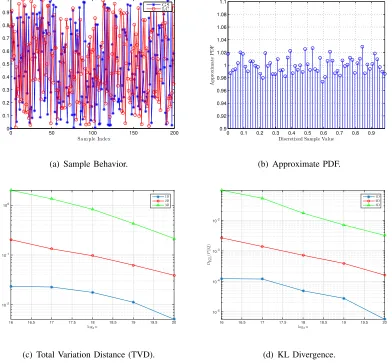
Though we are not able to prove Conject. 1, its correctness can be verified by simulations. Some examples are given in Fig. 1 to confirm Conject. 1 from different aspects. First, Fig. 1(a) shows that the samples of GS ceiling errors look very like the samples generated by the LC method. Second, Fig. 1(b) gives an approximateprobability density function (PDF) of GS ceiling errors to show that GS ceiling errors are uniformly distributed over[0,1). In addition, it can also be found from the caption of Fig. 1 that the mean and variance of GS ceiling errors are very close to those ofU(0,1), whereU(a, b)stands for the uniform distribution over[a, b), especially when there are a large number of samples.

Third, Figs. 1(c) and 1(d) give the total variation distance (TVD) and Kullback-Leibler divergence (KLD) of GS ceiling errors to show that GS ceiling errors can be taken as the samples of independent random variables. The TVD between probability distributions P and Q

is defined as δ(P, Q) := sup|p(x)−q(x)|, where p and q denote the densities of P and Q. The KLD of Q from P is defined as

DKL(PkQ) :=

Z ∞

−∞

p(x) log₂ p(x)

q(x)dx. (16)

To make the results more convincing, we study the TVD and KLD of GS ceiling errors from multiple dimensions. Let (e0, e1,· · ·)be a series of GS ceiling errors and q(xk)the “joint PDF”

of (ei,· · · , ei+k−1). If e0, e1,· · · are independent and uniformly-distributed (i.u.d.) over [0,1),

we haveq(xk_{) = 1for all x}k _∈[0,1)k_{. To verify this point, we let p(x}k_{) = 1 for allx}k _∈[0,1)k_.

Then the k-D TVD between P and Q becomes δ(P, Q) = sup_xk_∈[0,1)k|q(xk)−1| and the k-D

KLD of Q from P becomes

DKL(PkQ) :=−

Z 1 0

· · ·

Z 1 0

log₂q(xk)dx0· · ·dxk−1. (17)

To estimate q(xk_{), we discretize space [0,1)}k _{into m}k _{equal-size cells and count the number of}

GS ceiling errors falling within each cell. Then DKL(PkQ) can be approximated by

DKL(PkQ)≈ −(1/mk)

X

ik_∈[0:m)k

log₂q(ik/m). (18)

down, showing thatq(xk_{)tends to be uniform over[0,1)}k_{. Hence, GS ceiling errors can be taken}

as the samples of i.u.d. random variables.

Similar results are also obtained for other settings. According to the above observations, we assume that Conject. 1 is correct and use it in the following deduction. In addition, because flooring and rounding errors can be taken as the shifted versions of ceiling errors, for a GS with non-integer common ratio r > 1, flooring and rounding errors can be taken as the samples of i.i.d. random variables that are uniformly distributed over (−1,0] and (−0.5,0.5], respectively.

Assuming that Conject. 1 is true, then it is easy to prove the following conjecture.

Conjecture 2 [Ceiling Errors of Weighted Sum of Geometric Series] Let (a, ar, ar2,· · ·)

be a GS with initial term a and non-integer common ratio r > 1. Let Xn be a tuple of i.i.d. binary random variables andS =Pn−1

i=0 ariXi. LetU = (dSe −S). Then forn sufficiently large, U ∼ U(0,1) and U is weakly correlated with Xn_.

IV. APPROXIMATEHDSOF TAILLESSDAC

With the help of Conject. 1, this section will derive a fast method to compute the approximate value of ψn,R(d). We define a ternary variable wi := zi(1−2xi) ∈ T := {−1,0,1}. Clearly,

wi = 0 if zi = 0 and wi = ±1 if zi = 1. Conversely, if wi = ±1, we have zi = 1 and xi = (1− wi)/2; otherwise, i.e., wi = 0, we can get zi = 0, but xi is unknownable. Thus,

given wn_{, z}n _{is fully determined, but x}n _{is partially determined. Concretely speaking, each w}n

leads 2n−|wn_|

different xn_{’s. Further, we let Z ⊆ [0 : n) be the set of support indices of z}n

and Zc _{:= [0 : n)\ Z, i.e., z}

i = 1 if i ∈ Z and zi = 0 if i ∈ Zc. Thus |Z| = |zn| and

|Zc_{|=n− |z}n_{|. From x}n_{, we draw all elements indexed by Z to form a sub-vector x}

Z ∈B|z

n_|

. Similarly, xZc ∈_Bn−|z

n_|

is also formed. Now we define

τn,R(wn) := (1−2−R) n−1

X

i=0

wi2(n−i)R

= (1−2−R)X i∈Z

wi2(n−i)R. (19)

0 50 100 150 200 0 0.1 0.2 0.3 0.4 0.5 0.6 0.7 0.8 0.9 1

Sa m ple Index

S a m p le V a lu e G S LC

(a) Sample Behavior.

0 0.1 0.2 0.3 0.4 0.5 0.6 0.7 0.8 0.9

0.9 0.92 0.94 0.96 0.98 1 1.02 1.04 1.06 1.08 1.1

Discretized Sample Value

Ap p ro x im a te P D F

(b) Approximate PDF.

log2n

16 16.5 17 17.5 18 18.5 19 19.5 20

δ ( P ,Q ) 10-2 10-1 100 1D 2D 3D

(c) Total Variation Distance (TVD).

log2n

16 16.5 17 17.5 18 18.5 19 19.5 20 DK L ( P k Q ) 10-5 10-4 10-3 10-2 1D 2D 3D

(d) KL Divergence.

Fig. 1. (a) GS ceiling-error samples versus LC samples. The LC method is realized by the MATLAB functionrand(). The number of samples for each sequence is200. For the GS, the common ratio isr= 1.1and the initial term isa= 1. The mean of samples is0.4820for GS and0.4926for LC. The variance of samples is0.0885for GS and0.0789for LC. (b) Approximate PDF of GS ceiling errors. The common ratio isr = 1 + 10−4 and the initial term is a = 100. We collect218 samples and discretize interval[0,1)intom= 64cells. The mean of samples is0.5, the same as the mean of U(0,1), and the variance is

0.0834, close to 1/12 = 0.0833, the variance of U(0,1). (c) and (d) TVD and KLD of GS ceiling errors, respectively. The initial term isa= 1010and the common ratio isr= 1 + 10−5. The number of samplesnvaries from216to 220. The space

[0,1)k is divided intomk equal-size cells, wherem= 16.

A. Root Coexisting Interval

Obviously, if only wn and xZc are known, xn and zn can be deduced exactly. Hence, we

rewrite I(xn_{, z}n_{) as I(w}n_{, x}

Zc) and define

  

δ−(wn) :=1τn,R(wn_)<0·min(1,|τ_n,R(wn)|)

δ+(wn) :=1τn,R(wn_)>0·min(1,|τ_n,R(wn)|)

It is easy to see that δ−(wn_{) +δ}+_(wn_{)≡min(1,|τ}

n,R(wn)|)≤1 and δ−(wn)·δ+(wn)≡0. We

can now rewrite (10) as

I(wn, xZc) = (m(xn)−1) +δ−(wn), m(xn)−δ+(wn)

= {m(xn)− I(wn)}, (21)

where

I(wn) :=

δ+(wn),1−δ−(wn)

⊆[0,1). (22)

We call I(wn) the wn-root coexisting interval. Obviously, there are |_Tn_{| = 3}n _{root coexisting}

intervals in total. Since I(wn_{, x}

Zc) is a shifted version of I(wn), each root coexisting interval

in fact leads 2n−|wn_|

coexisting intervals. Clearly, I(wn_{) = ∅ if |τ}

n,R(wn)| ≥ 1 and for all xZc ∈_Bn−|w

n_|

,

|I(wn, xZc)|=|I(wn)|= (1− |τn,R(wn)|)+. (23)

Coexisting Interval versus Risky Interval In [20], the concept ofrisky intervalwas proposed,

which is similar to the coexisting interval to some extent. Below we discuss their differences. A risky interval can be denoted by I(xZ)

m,Z, where m∈[0 : 2nR) is codebook index. It is obvious

that given xn _{6= 0}n_{, I(w}n_{) = 1− I}(xZ)

1,Z . It is proved in [20] that given Z and xZ, |I_m,(xZZ)|’s are

the same for all m ∈[1 : 2nR_{). As a sub-vector of x}n_{, x}

Z in fact leads 2n−|z

n_|

different xn_{’s. It}

can be easily shown that given xn_{6= 0}n_{, for all x}

Zc ∈_Bn−|z n_|

,

I(wn, xZc)∈ {I(xZ)

m,Z :m∈[1 : 2

nR

)}. (24)

B. Approximate Expression of HDS

With wn _{and x}

Zc, we can obtain

ψn,R(d) = 2−d

X

wn_:|wn_|=d

ρ(wn), (25)

where

ρ(wn) := 2−(n−d) X xZc∈_Bn−d

1I(wn_,x

Zc)(s(xn)). (26)

According to (21), we have

1I(wn_,x

Let us rewrite (2) as

s(xn) = (1−2−R) X i∈Z

(1−wi)2(n−i)R−1+

X

i∈Zc

xi2(n−i)R

!

= c(Z) +ϕ(xZc)−τ_n,R(wn)/2, (28)

where

      

c(Z) := (1−2−R)X i∈Z

2(n−i)R−1

ϕ(xZc) := (1−2−R)

X

i∈Zc

xi2(n−i)R

. (29)

Similarly, we can obtain

s(xn⊕zn) = c(Z) +ϕ(xZc) +τn,R(wn)/2. (30)

Note the following three points:

• (m(xn)−s(xn))∈[0,1) is actually the ceiling error ofs(xn);

• for each given wn, both c(Z) and τ_n,R(wn) are fixed for all x_Zc ∈_Bn−|w n_|

;

• ϕ(x_Zc) is the partial sum of a geometric series.

According to Conject. 1, we affirm that (m(xn)−s(xn))’s for different xZc ∈_Bn−|w n_|

perform like the samples of i.i.d. random variables that are uniformly distributed over [0,1). Hence for a given wn_{, if there are a large number of x}

Zc’s, ρ(wn)will be approximately equal to the ratio

of the length of I(wn_{) to that of [0,1), i.e.,}

ρ(wn)≈ |I(wn)|= (1− |τn,R(wn)|)+. (31)

Finally, we obtain

ψn,R(d)≈2−d

X

wn_:|wn_|=d

(1− |τn,R(wn)|)+. (32)

Given |wn_{| = d, there are} n d

2d _{different w}n_{’s, so the complexity of computing ψ}

n,R(d) via

(32) is O( n_d

2d_{). Since} Pn

d=0 n d

2d _{= 3}n_{, the total complexity of computing all ψ}

n,R(d)’s for d ∈ [0 : n] via (32) is O(3n), which is, for large n, far lower than O(4n). As for calculating

τn,R(wn), it can be found from (19) that the complexity is O(n). It is easy to find that (32) is

in fact equivalent to equation (46) in [20]. However, it must be pointed out that (31) holds only when (n− |wn_{|) is large, i.e., there are a large number of distinct x}

Zc’s, because ρ(wn) is the

average of 2n−|wn_|

C. Case of Small (n− |wn_|)

Given wn, the number of distinct xZc’s is 2n−|w n_|

, decreasing as|wn|goes up. For (n− |wn|)

not very large, there are only a few distinctxZc’s, so |I(wn)| may not be a good approximation

of ρ(wn_{) in this case. Nevertheless, if only n is sufficiently large, ψ}

n,R(d) for any d < n can

still be well approximated by (32) because its right side is the sum of n_d2d _{pseudo-independent}

terms. However, ψn,R(n) is still hard to find. If |wn| = n, we have zn = 1n, Z = [0 : n), and

Zc _{=∅. Thus, ϕ(x}

Zc) = 0 and

c(Z) = (1−2−R) n

X

i=1

2iR−1 = (2nR−1)/2. (33)

We can then obtain

(

s(xn) = 2nR−1−(1 +τn,R(wn))/2

s(xn⊕zn) = 2nR−1−(1−τn,R(wn))/2

. (34)

If |τn,R(wn)|<1, (1±τn,R(wn))/2∈(0,1) and hence for any nR∈Z,

m(xn) =m(xn⊕zn) = 2nR−1 ∈_Z, (35)

i.e., xn _{and (x}n_⊕zn_{) always belong to the 2}nR−1_{-th codebook. Thus if |w}n_|=n,

ρ(wn) =1|τn,R(wn_)|<1 =1_|τn,R(xn_,1n_)|<1 ∈_B, (36)

showing that ρ(wn_{) cannot be approximated by (1− |τ}

n,R(wn)|)+. Now we get ψn,R(n) = 2−n

X

xn_∈

Bn

1|τn,R(xn_,1n_)|<1. (37)

Sinceψn,R(n)is the average of 2n binary terms, we haveψn,R(n)<1. According to (34), given

|wn_{|=n, if |τ}

n,R(wn)|<1, s(xn)∈((2nR−1−1),2nR−1), and vice versa. Hence,

1|τn,R(xn_,1n_)|<1 =1₍₍₂nR−1_−1),2nR−1₎(s(xn)). (38)

According to (37) and (38), we can obtain

ψn,R(n) = Pr s(Xn)∈((2nR−1−1),2nR−1)

. (39)

According to Conject. 1, given|τn,R(wn)|<1, |τn,R(wn)|is approximately uniformly distributed

over [0,1) for nR sufficiently large. Therefore,

X

xn_∈

Bn

(1− |τn,R(xn,1n)|)+

!

≈ 1

2

X

xn_∈

Bn

1|τn,R(xn_,1n_)|<1

!

, (40)

showing that the approximate value of ψn,R(n) given by (32) is roughly half of its exact value

V. HDSOFTAILEDDAC

A. Review of Tailed DAC Encoding

Tailed DAC divides each source blockxn_{into bodyx}n−t_{and tailx}n

n−t. Let us use the(n, R, t)

DA code to stand for a tailed DA code with lengthn, rateR, and tail lengtht. Each tail symbol is always coded at rate 1, so the mapping rule is: 0 →[0,2−1_{) and 1 →[2}−1_{,1). To compress} xn at the average rate R, each body symbol should be coded at rate r = nR_n−−_tt ≤ R, so the mapping rule is: 0→[0,2−r) and1→[(1−2−r),1). It is easy to get(n−t)(1−r) =n(1−R). To guarantee r ≥ 0, t must not be larger than nR, so t ∈ [0 : nR]. (Obviously, tailless DAC is a special form of tailed DAC obtained by setting t = 0 and r =R.) The final interval after coding xn _{is still [l(x}n_{), l(x}n_{) + 2}−nR_{), where}

l(xn) = (1−2−r) n−t−1

X

i=0

xi2−ir+ n−1

X

i=n−t

xi2n(1−R)−1−i. (41)

Because nR= (n−t)r+t, we have

s(xn) = 2t(1−2−r) n−t−1

X

i=0

xi2(n−t−i)r+ n−1

X

i=n−t

xi2n−1−i. (42)

The scaled final interval is still [s(xn_{), s(x}n_{) + 1) and s(x}n_{) ≤ (2}nR_{−1). It can also be seen}

that m(xn_{)∈[0 : 2}nR_{) still holds.}

B. Calculation of HDS for Tailed DAC

According to the definition of τn,R(wn), we can obtain

τn,R(wn) = 2t(1−2−r) n−t−1

X

i=0

wi2(n−t−i)r+ n−1

X

i=n−t

wi2n−1−i

= 2tτn−t,r(wn−t) +τt,1(wnn−t). (43)

The exact and approximate values of ψn,R(d) can be computed via (15) and (32), respectively.

An Extreme Case. When t = nR, r = (1−2−r_{) = 0, so τ}

n,R(wn) = τt,1(wnn−t) ∈ Z, i.e., τn,R(wn)purely depends onwnn−t and is always an integer. Thus, ifznn−t 6= 0t, xn and (xn⊕zn)

cannot coexist in the same codebook, i.e., ψn,R(d) = 0 for d >(n−t) = n(1−R). In addition,

since τn,R(wn) is not related to wn−t, it is easy to see that, when t=nR,

ψn,R(d) =

  

n(1−R) d

, d∈[0 :n(1−R)]

0, d∈(n(1−R) :n]

C. Removal of Closely-Spaced Fellow Codewords

Though experiments show that tailed DAC is better than tailless DAC [3], [4], there is no theoretical explanation on the superiority of tailed DAC over tailless DAC. Below, we will reveal that closely-spaced fellow codewords can be removed by increasing tail length, which explains the superiority of tailed DAC over tailless DAC. Due to computation complexity and to keep the exposition simple, we consider below only two special cases ψn,R(1) and ψn,R(2). To begin

with, we give the following claim.

Claim 1 If |zn−t_{| = 0 and |z}n

n−t| >0, then m(xn) 6=m(xn⊕zn). Conversely, if |zn|> 0 and m(xn_{) =m(x}n_⊕zn_{), then |z}n−t_|>0.

In plain words, if a pair of codewords coexist in the same codebook, it is impossible that these two codewords differ from each other only in tails. The proof of Claim 1 is obvious and is omitted. With the help of Claim 1, we explain below why ψn,R(1) and ψn,R(2) will tend to 0 as t increases. Then, we discuss the general case of ψn,R(d) when d >2.

1) 1-Away Fellow Codewords: Given |wn| = 1, there are two sub-cases: |wn−t| = 0 and |wn

n−t| = 1; |wn

−t_{| = 1 and |w}n

n−t| = 0. According to Claim 1, in the former sub-case, it is

certain that m(xn_{) 6= m(x}n_⊕zn_{). Hence, we need to consider only the later sub-case, which}

means τn,R(wn) = 2tτn−t,r(wn−t). Given |wn−t|= 1, we can obtain from (43) that

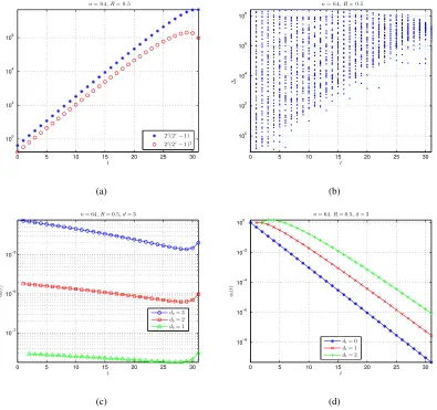
|τn−t,r(wn−t)| ≥(1−2−r)2r = (2r−1) (45)

and further |τn,R(wn)| ≥ 2t(2r−1). Suppose that t ≤ nR₂ . Then r ≥ ₂₋R_R. Hence 2t(2r−1)≥ 2t₍₂2−RR−1)_{. For large}n_{, increasing} t _{will make}2t(2

R

2−R −1)≥1_{. An example of}2t(2r−1)_is

given in Fig. 2(a) for n= 64 and R= 0.5, which shows that2t₍₂r_{−1)increases monotonously}

for small t. Hence, it is possible to make |τn,R(wn)| ≥ 1, i.e., I(wn) = ∅, hold always for

all wn_{’s satisfying |w}n_{| = 1 by increasing t. In other words, 1-away fellow codewords can be}

removed by simply increasing tail length t, even for finite code length n.

2) 2-Away Fellow Codewords: Given |wn_{| = 2, there are three sub-cases: |w}n−t_{| = 0 and}

|wn

n−t|= 2; |wn

−t_{|= 2 and |w}n

n−t|= 0; |wn

−t_|=|wn

n−t|= 1. According to Claim 1, in the first

sub-case, m(xn)6=m(xn⊕zn), so we need to consider only the later two sub-cases. In the sub-case of |wn−t_{|= 2 and |w}n

to get from (43) that, given |wn−t_{|= 2,}

|τn−t,r(wn−t)| ≥(1−2−r)(22r−2r) = (2r−1)2. (46)

Thus, given|wn−t_{|= 2and|w}n

n−t|= 0,|τn,R(wn)| ≥2t(2r−1)2. Still suppose thatt≤ nR₂ , which

is followed by2t₍₂r₋₁₎2 _≥2t₍₂2−RR−1)2. For largen, increasingt will make2t(2 R

2−R−1)2 ≥1,

as shown by Fig. 2(a), where n= 64 and R = 0.5. Hence, it is possible to make |τn,R(wn)| ≥ 2t(2r−1)2 ≥1, i.e., I(wn) =∅, hold always for all wn’s satisfying |wn−t|= 2 and |wn_n−t|= 0

by increasing tail length t. In the sub-case of|wn−t_|=|wn

n−t|= 1, we have|τn−t,r(wn−t)|= (2r−1)2irfori∈[0 : (n−t))

and|τt,1(wnn−t)|= 2j forj ∈[0 :t). Letγi := (2r−1)2t+ir. Then, we have|τn,R(wn)|=|γi±2j|,

where (i, j) ∈ [0 : (n−t))×[0 : t). Since γi > 0 for all i ∈ [0 : (n−t)) and 2j ≥ 1 for all j ∈ [0 : t), |γi + 2j| > 1 holds always. Thus, it is unnecessary to consider |γi + 2j|. As for

|γi −2j|, there are (n−t)×t possible values for (i, j) ∈ [0 : (n−t))×[0 : t). For n very

large and t n, r≈ R and thus (γi+1−γi) increases w.r.t. t, i.e., γi’s tend to be sparser as t

increases. Hence as tincreases, it is less likely thatγi’s fall within(2j−1,2j+ 1)’s. An example

is given in Fig. 2(b) to confirm this point, where

∆i := min(γi−2blog2γic,2dlog2γie−γi). (47)

As shown by Fig. 2(b), as t increases, fewer ∆i’s will be less than 1 and when t > 6, there is

no ∆i less than 1. Therefore, it is possible to make|τn,R(wn)|=|γi±2j| ≥1, i.e., I(wn) = ∅,

hold always for all wn_{’s satisfying |w}n−t_|=|wn

n−t|= 1 by increasing t.

Based on the above analyses, we conclude that 2-away fellow codewords can be removed by simply increasing tail length t, even for finite code length n.

3) General Case: The analysis of the general case d >2 is more complex, but the principle is similar to the above cases. From (43), we have

|τn,R(wn)|=

  

2t|τ_n−t,r(wn−t)| − |τt,1(wnn−t)|

, τ_n−t,r(wn−t)·τt,1(wnn−t)<0 2t|τn−t,r(wn−t)|+|τt,1(wnn−t)|, τn−t,r(wn−t)·τt,1(wnn−t)≥0

. (48)

From (19), we have |τn−t,r(wn−t)| ∈ [0,(2(n−t)r−1)] and |τt,1(wnn−t)| ∈ [0 : 2t) ⊂ Z. Further, 2t_|τ

n−t,r(wn−t)| ∈[0,(2nR−2t)] and |τn,R(wn)| ∈[0,(2nR−1)]. Therefore,

2t|τn−t,r(wn−t)|,|τt,1(wnn−t)|

0 5 10 15 20 25 30 100

102 104 106

t n_{= 6 4 ,}R_{= 0}.₅

2t (2r

−1 ) 2t

(2r −1 )2

(a)

0 5 10 15 20 25 30

100 102 104 106 108

t

∆

i

n= 6 4 ,R= 0.5

(b)

0 5 10 15 20 25 30

10−7 10−6 10−5

t φb

(

t

)

n= 64,R= 0.5,d= 3

db= 3

db= 2 db= 1

(c)

0 5 10 15 20 25 30

10−8 10−6 10−4 10−2 100

t φt

(

t

)

n= 64,R= 0.5,d= 3

dt= 0

dt= 1

dt= 2

(d)

Fig. 2. (a)2t(2r−1)and 2t(2r−1)2 versus tail lengtht. (b) Distribution of∆i, defined by (47), versus tail lengtht. (c) Conditional body density. (d) Conditional tail density.

Given |wn_n−t|>0, we have

2t|τn−t,r(wn−t)|+|τt,1(wnn−t)| ≥ |τt,1(wnn−t)| ≥1. (50)

Thus, we need to consider only the sub-case of

|τn,R(wn)|=2t|τn−t,r(wn−t)| − |τt,1(wnn−t)|

. (51)

The conditional “density” of 2t_|τ

n−t,r(wn−t)| over [0,(2nR−2t)] given |wn−t|= db ≤ (n−t),

which will be referred to as conditional body density for brevity, is defined as

φb(t) := |{w

n−t_:|wn−t_|=d b}|

2nR₋₂t =

n−t db

2db

It is easy to see that

n−(t+ 1) db

= n−t−db n−t

n−t db

= (1− db

n−t)

n−t db

. (53)

Since (2nR−2t+1) = (2nR−2t−2t), we have

2nR−2t+1

2nR₋₂t = 1− 2t

2nR ₋₂t = 1− 1

2nR−t₋₁. (54)

Thus,

φb(t+ 1) = 1− db n−t

1− 1

2nR−t₋₁

φb(t). (55)

Note the following two points:

• Both db

n−t and 1

2nR−t₋₁ are monotonously-increasing and convex over t∈[0 :nR];

• For nR large enough, db

n−t|t=0 = db

n > 1

2nR−t₋₁|t=0 = 1

2nR₋₁, and db

n−t|t=nR = db n(1−R) < 1

2nR−t₋₁|t=nR =∞.

Hence, there must exist t∗ ∈ [0, nR] ⊂ _R that makes _ndb_−t∗ =

1

2nR−t∗₋₁, and db n−t >

1 2nR−t₋₁

for t < t∗ and _ndb_−t < 1

2nR−t₋₁ for t > t

∗

. Further, we have φb(t+ 1) < φb(t) for t < t∗ and φb(t + 1) > φb(t) for t > t∗, i.e., φb(t) is monotonously decreasing over t ∈ [0 : dt∗e] and

monotonously increasing over t ∈ [dt∗e : nR]. Some examples of φb(t) are given in Fig. 2(c),

which show that t∗ is usually very close to nR.

The conditional “density” of |τt,1(wnn−t)| over [0 : 2t) given |wnn−t| = dt ≤ t, which will be

referred to as conditional tail density for brevity, is defined as

φt(t) :=

|{w_nn_−t:|w_nn_−t|=dt}|

2t =

t dt

2dt

2t =

t dt

2dt−t. (56)

Hence, φt(t + 1) = _2(t−t+1_dt+1)φt(t). It is easy to see that _2(t−t+1_dt+1)|t=2dt−1 = 1, i.e., φt(2dt) = φt(2dt − 1). Thus, φt(t) is monotonously increasing over t ∈ [dt : 2dt) and monotonously

decreasing over t∈[2dt:nR]. Some examples ofφt(t) are given in Fig. 2(d).

Since both φb(t) and φt(t) decrease monotonously over t ∈ [2dt : dt∗e], 2t|τn−t,r(wn−t)|

(|τt,1(wnn−t)|, resp.) will tend to be sparser over [0,(2nR −2t)] ([0 : 2t), resp.) as t increases.

Further, from the statistical viewpoint,2t|τn−t,r(wn−t)| − |τt,1(wnn−t)|

will tend to be larger as t

increases. Thus, it is possible to make|τn,R(wn)| ≥1for allwn’s satisfying|wn|=d=db+dt n by increasing t. In other words, for n sufficiently large and d n, ψn,R(d) will tend to 0

as t increases. However, note that as d increases, larger t is required to make ψn,R(d) = 0. For

example, Fig. 2 shows thatψn,R(1) = 0 when t >1, but t >6is required to make ψn,R(2) = 0.

VI. CODEBOOK CARDINALITY SPECTRUM

A. Definitions

The projection of m(Xn) onto [0,2nR) ⊂ _R is U0,n := 2−nRm(Xn) ∈ [0,1). We define the

level-i projection of bitstream m(Xn) as Ui,n =ui(Xn), where

ui(Xn) :=

  

2ir U0,n−l(Xi)

, i∈[0 : (n−t)]

2i−n(1−R) U0,n−l(Xi)

, i∈[(n−t) :n]

. (57)

We callU0,n the initial bitstream projection andUn,n the final bitstream projection. Note thatUi,n

is defined over[0,1)⊂_R, so its pdf exists and is called the level-iCCS. Let us denote the level-i

CCS by f_n,R,t(i) (u). Especially, the subscript t can be dropped if t = 0, i.e., f_n,R(i) (u) =f_n,R,(i) ₀(u). The conditional pdf of Ui,n givenXj =xis called the conditional level-iCCS givenXj =xand

denoted by f_n,R,t(i,j)(u|x). The subscript t can be dropped if t = 0, i.e., f_n,R(i,j)(u|x) = f_n,R,(i,j)₀(u|x). To simplify notation, f_n,R,t(i,i) (u|x) is abbreviated to f_n,R,t(i) (u|x).

B. Calculation of CCS

Below, we derive f_n,R,t(n) (u) based on Conject. 2. Since Un,n =m(Xn)−s(Xn),

fUn,n|Xn(u|xn) =δ(u−(m(xn)−s(xn))), (58)

where fUn,n|Xn(u|xn) is the conditional pdf of U_n,n given Xn=xn and δ(u) is the Dirac delta

function. Therefore,

f_n,R,t(n) (u) = X xn_∈

Bn

Pr(Xn =xn)δ(u−(m(xn)−s(xn)))

= 2−n X

xn_∈

Bn

δ(u−(m(xn)−s(xn))). (59)

As shown by Conject. 2, (m(xn_)−s(xn_{))’s for different x}n_{’s perform like the samples of i.i.d.}

random variables that are uniformly distributed over [0,1). Thus, for n sufficiently large, Un,n

is weakly correlated with Xn and f_n,R,t(n) (u)≈Π(u), where

Π(u) :=

(_{1, 0≤u <1}

0, u <0 or u≥1

. (60)

According to (57), for i∈[(n−t) :n),

Ui,n=Ui+1,n/2 +Xi/2 =Un,n2i−n+ n−1

X

i0_=i

Xi02(i−i 0₎₋₁

For n sufficiently large, Un,n is weakly correlated with Xn, so Ui,n, the weighted sum of Un,n

andX_in, is weakly correlated withXi (note that Xi is independent ofX_in). Thus, the pdf ofUi,n

is the convolution of the pdf of Ui+1,n/2 and that of Xi/2. Since aXi ∼ 1₂(δ(x) +δ(x−a)),

f_n,R,t(i) (u) ≈ 2f_n,R,t(i+1)(2u)⊗ δ(u) +δ(u−2−1)2−1

= f_n,R,t(i+1)(2u) +f_n,R,t(i+1)(2u−1). (62)

where ⊗ denotes the convolution operation. We can then obtain f_n,R,t(i) (u) ≈ f_n,R,t(n) (u) ≈ Π(u)

for all i∈[(n−t) :n).

As for i∈[0 : (n−t)), it is easy to see that f_n,R,t(i) (u)≈f_n(i−)t,r(u), where r = nR

−t

n−t , i.e., the

level-i CCS of the (n, R, t) tailed DA code approximates to the level-i CCS of the (n−t, r)

tailless DA code, so we will discuss only the (n, R)tailless DA code below. According to (57),

Ui,n =Ui+1,n2−R+ (1−2−R)Xi =Un,n2(i−n)R+ (1−2−R) n−1

X

i0_=i

Xi02(i−i 0_)R

. (63)

It can be seen that, for n sufficiently large, Ui,n is weakly correlated with Xi and

f_n,R(i)(u) ≈ 2Rf_n,R(i+1)(u2R)⊗ δ(u) +δ(u−(1−2−R))2−1 =

f_n,R(i+1)(u2R) +f_n,R(i+1)(u2R−(2R−1))

2R−1

≈ Π(u2(n−i)R)⊗λn−i,R(u)

2(n−i)(R−1), (64)

where

λn0,R(u) :=

n0₋₁

O

i0₌₀

δ(u) +δ(u−(1−2−R)2−i0R)

= X

xn0_∈

Bn0

δ(u−l(xn0)). (65)

It is interesting that2−nλn,R(u)is actually the pdf ofl(Xn). Sincelimn→∞2nRΠ(u2nR) =δ(u),

for n sufficiently large and in, we have f_n,R(i) (u)≈λn−i,R(u)≈λ∞,R(u).

C. Conditional CCS

Forn sufficiently large, Ui,n is weakly correlated withXi, so for the(n, R)tailless DA code, f_n,R(i,j)(u|x)≈f_n,R(i) (u) for i > j. As for f_n,R(i)(u|x), we have

f_n,R(i)(u|x) ≈ 2Rf_n,R(i+1,i)((u2R−x(2R−1))|x)

It is obvious that

f_n,R(i)(u) =X x∈_B

Pr(Xi =x)f (i)

n,R(u|x) = 1 2

X

x∈_B

f_n,R(i) (u|x). (67)

Let pi(x|u) := Pr(Xi =x|Ui,n=u). According to Bayes’ theorem, we can obtain

pi(x|u) =

Pr(Xi =x)f (i) n,R(u|x) f_n,R(i) (u) =

f_n,R(i)(u|x)

2f_n,R(i)(u). (68)

VII. ACCANDRATE LOSS OFTAILEDDAC

With the help of CCS, we will derive below the ACC and rate loss of tailed DAC, which is helpful for us to understand the properties of DA codes. The deduction of ACC is rather simple. According to the analyses in [19], it is easy to show that the ACC of the (n, R, t) tailed DA code is approximately η2n(1−R)_{, where}

η :=

Z 1

0

f_n,R,t(0) (u) 2

du. (69)

We call η the ACC scaling factor. Obviously, η ≥ 1 and the equality holds only if f_n,R,t(0) (u) = Π(u). On the contrary, the deduction of rate loss is much more difficult, as shown below.

A. Deduction of Rate Loss

Since f_n,R,t(0) (u)≈f_n(0)−t,r(u), only the (n, R) tailless DA code is considered in this subsection

for simplicity. We deduce H(Xn_|m(Xn_{)) first, which measures the remaining uncertainty of} Xn _{given m(X}n_{). Since m(X}n_{) is a deterministic function w.r.t. X}n_{, we have H(X}n_{) =} H(m(Xn_{)) + H(X}n_|m(Xn_{)). Because m(X}n_{) ∈ [0 : 2}nR_{), we have H(m(X}n_{)) ≤ nR and}

the equality holds only if m(Xn) is uniformly distributed over [0 : 2nR). Further, because

U0,n = 2−nRm(Xn), we have H(Xn|m(Xn)) = H(Xn|U0,n).

Lemma VII.1 (Decomposition of Conditional Entropy). For n sufficiently large,

H(Xn|m(Xn)) =H(Xn|U0,n)≈ n−1

X

i=0

H(Xi|Ui,n). (70)

Proof: By the chain rule, we can get

H(Xn|U0,n) = n−1

X

i=0

H(Xi|U0,n, Xi) (a)

= n−1

X

i=0

where (a) is because Xn _{is the tuple of i.i.d. random variables. Further, because U}

i,n is weakly

correlated with Xi for n sufficiently large, it can be seen that U0,n, Ui,n, and Xi approximately

form a Markov chain. Thus, H(Xi|U0,n)≈H(Xi|Ui,n) for n sufficiently large.

Lemma VII.2 (Symbol-wise Rate Loss). Let h(·) denote the differential entropy. For n

suffi-ciently large, the rate loss of coding Xi with the (n, R) tailless DA code is

H(Xi|Ui,n)−(1−R)≈h(Ui+1,n)−h(Ui,n). (72)

Proof: It is easy to show that

H(Xi|Ui,n) =

Z 1

0

f_n,R(i)(u)H(Xi|Ui,n =u)du, (73)

where

H(Xi|Ui,n=u) =−

X

x∈_B

pi(x|u) log2pi(x|u). (74)

By substituting (68) into (74), we obtain

f_n,R(i) (u)H(Xi|Ui,n=u) = −f (i) n,R(u)

X

x∈B

pi(x|u) log2pi(x|u)

= −1

2

X

x∈B

f_n,R(i) (u|x)log₂f_n,R(i) (u|x)−1−log₂f_n,R(i)(u) (a)

= f_n,R(i)(u)1 + log₂f_n,R(i)(u)− 1

2

X

x∈B

f_n,R(i)(u|x) log₂f_n,R(i) (u|x)

!

,

(75)

where (a) comes from f_n,R(i) (u) = 1₂P

x∈Bf

(i)

n,R(u|x). Further,

H(Xi|Ui,n) = 1−h(Ui,n) + 1 2

X

x∈B

h(Ui,n|Xi =x). (76)

According to the properties of differential entropy and (66), h(Ui,n|Xi = x) ≈ h(Ui+1,n)−R

for n sufficiently large. Hence,

H(Xi|Ui,n) ≈ 1−h(Ui,n) +h(Ui+1,n)−R

= (1−R) + (h(Ui+1,n)−h(Ui,n)). (77)

According to Lem. VII.2, it is obvious that h(Ui,n) is monotonically increasing w.r.t. i. Since f_n,R(i)(u) is defined over [0,1), we have h(Ui,n)≤0 and the equality holds iff Ui,n is

uniformly-distributed over [0,1). Therefore, h(U0,n) ≤ · · · ≤h(Un,n)≤0. As (n−i)→ ∞, both f (i) n,R(u)

and f_n,R(i+1)(u) will converge to f_∞(0)_,R(u) and thus (h(Ui+1,n)−h(Ui,n)) → 0. Hence, for each xn _∈

Bn, the symbols far from the end can be compressed near-losslessly with the (n, R) DA

code, and the rate loss comes mainly from ending symbols.

Theorem VII.3 (Block-wise Rate Loss). For n sufficiently large, the total rate loss of coding

Xn _{with the (n, R) tailless DA code is}

H(Xn|m(Xn))−n(1−R)≈ −h(U0,n). (78)

Proof: Based on Lems. VII.1 and VII.2, it is easy to obtain

H(Xn|m(Xn)) =H(Xn|U0,n)≈n(1−R) +h(Un,n)−h(U0,n). (79)

Sincem(Xn)is represented bynR bits, the remaining uncertainty ofXn givenm(Xn)is lower bounded by H(Xn)−nR= n(1−R). Thus, the total rate loss of coding Xn with the (n, R)

tailless DA code is H(Xn_|m(Xn_{))−n(1−R) = h(U}

n,n)−h(U0,n). For n sufficiently large, Un,n is almost uniformly distributed over [0,1) and thus h(Un,n)≈0.

B. Physical Meaning of Rate Loss

The rate loss of DA codes can be explained intuitively with an example. We first compress

Xn _{with the (n, R) DAC encoder to obtain bitstream m(X}n_{) and then compress X}n _{with the}

standard AC encoder parameterized with the probability set{pi(x|u)}to obtain another bitstream

ˆ

m(Xn). Obviously, the length of m(Xn) is always nR and the expected length of mˆ(Xn) is aboutn(1−R)−h(U0,n). Thus, the total length of m(Xn)andmˆ(Xn)is aboutn−h(U0,n)> n.

It can be shown that the error-free recovery of Xn _{is achievable by the interaction between the}

DAC decoder of m(Xn_{) and the standard AC decoder of mˆ(X}n_{). First, according to U}

0,n, the

DAC decoder can obtain p0(x|u), which is used by the AC decoder to recoverX0 exactly. Next according to U0,n and X0, the DAC decoder can obtain U1,n and p1(x|u), which is then used

by the AC decoder to recoverX1 exactly. Such operations are repeated until Xn−1 is recovered.

This example shows that Xn _{can be exactly represented by two bitstreams m(X}n_{)and mˆ(X}n_),

C. Effects of Tail Length

Now we discuss the effect of tail length t on the ACC and rate loss of DA codes. The initial CCS of the (n, R, t) tailed DA code is approximate to that of the (n−t, r) tailless DA code, where r= nR_n−−_tt, so for the (n, R, t) tailed DA code, the ACC scaling factor is

η≈

Z 1

0

f_n(0)_−t,r(u) 2

du (80)

and the rate loss is

−h(U0,n)≈

Z 1

0

f_n(0)_−t,r(u) log₂f_n(0)_−t,r(u)du. (81)

Note that f_n(0)−t,r(u) is subject to two parameters, t and r, that depend on each other, so both η

and −h(U0,n) behave strangely w.r.t. t.

We discuss the case of tnRfirst. Experiments show that f_n(0)0_,r(u) converges very fast asn0 increases, so f_n(0)_−t,r(u)≈f∞(0),r(u)for tnR. Thus givent nR, the ACC and rate loss of the

(n, R, t)tailed DA code almost purely depends on r, the coding rate of body symbols. It is easy to see that f∞(0),r(u) tends to be spikier as r decreases. Two extreme cases are f∞(0),1(u) = Π(u)

and f∞(0),0(u) =δ(u−0.5)[18]. Hence, both η and −h(U0,n) are monotonously decreasing w.r.t. r. For example, in the extreme case of r = 1, we have η = 1 and −h(U0,n) = 0; while in the

other extreme case of r = 0, we have η =−h(U0,n) =∞. Further, because r is monotonously

decreasing w.r.t. t, both η and −h(U0,n) of the (n, R, t) DA code are monotonously increasing

w.r.t. t nR. Thus, from the viewpoint of decoding complexity, increasing tail length t will cause a negative effect.

Next we consider the case of t ≈ nR. According to the definition of r, for small (nR−t),

r is very sensitive to t, so f_n(0)−t,r(u) cannot be approximated by f (0)

∞,r(u). Instead, for t ≈ nR,

f_n(0)−t,r(u)will tend to be flatter as t increases (cf. Fig. 5(a) in Sect. IX), meaning that both ACC

and rate loss will become smaller. In the extreme case of t =nR, we have f_n(0)_−t,r(u) ≈ Π(u),

η = 1, and −h(U0,n) = 0, hence the ACC is equal to 2n(1−R) and there is no rate loss. The

reason for this point is: When t = nR, xn

n−t is transmitted in its uncoded form, while xn

−t _is

not transmitted. These analyses will be further verified by experiments in Sect. IX.

VIII. NUMERICAL CALCULATION OF ACCANDRATELOSS

To obtain η and −h(U0,n), one must know f (0)

n,R,t(u) first. Since f (0)

n,R,t(u)≈f (0)

calculatef_n,R(0)(u) directly by (64) as it involves the convolution of a lot of terms, so we propose a numerical algorithm below. To begin with, the interval[0,1)is discretized into N equal-length cells. For N sufficiently large, f_n,R(i) (u) for u∈[0,1) can be approximated byf_n,R(i) (k/N), where

k ∈ [0 : N). For simplicity, f_n,R(i)(k/N) will be abbreviated to f_n,R(i)(k), while the meanings of

f_n,R(i)(k|x)andpi(x|k)are similar. Initially,f (n)

n,R(k)≡1for allk ∈[0 :N). LetH = rnd(N2

−R₎

and L= (N−H). First, we calculate

f_n,R(i)(k|x) =

  

f_n,R(i+1)(rnd((k−xL)2R)), k∈ {xL+ [0 :H)}

0, k∈ {(1−x)H+ [0 : L)}

. (82)

Then f_n,R(i)(k|x) is normalized by

f_n,R(i)(k|x) = N f_n,R(i)(k|x)

,_N−1 X

k=0

f_n,R(i)(k|x). (83)

Next we obtain f_n,R(i)(k) = 1₂P

x∈_Bf

(i)

n,R(k|x) and pi(x|k) = f (i)

n,R(k|x)/(2f (i)

n,R(k)). Finally, the

ACC scaling factor can be obtained through

η≈ 1

N N−1

X

k=0

f_n,R(0)(k) 2

(84)

and the block-wise rate loss can be obtained through

−h(U0,n)≈ 1 N

N−1

X

k=0

f_n,R(0)(k) log₂f_n,R(0)(k). (85)

In fact, the above numerical algorithm is very similar to the one proposed in [18], except that the clip operation, which bounds rnd((k−xL)2R_{) to be within [0 :N), is ignored in (82). Let}

us first explain why the clip operation in (82) is unnecessary for the case of x = 0. In (82), if

x = 0, we have 0 ≤ rnd(k2R) ≤ rnd((H −1)2R) for k ∈ [0 : H). Since H = rnd(N2−R), we have (H −N2−R_{) ∈ (−0.5,0.5] and further (H−1) ≤ (N2}−R_{−0.5), which is followed}

by (H −1)2R _{≤ (N −2}R−1_{). Since 2}R−1 _{∈ (0.5,1) for R ∈ (0,1), we have (N −2}R−1_{) ∈} (N −1, N −0.5). Therefore,

0≤rnd(k2R)≤rnd((H−1)2R)≤rnd(N −2R−1)< N, (86)

showing that rnd(k2R_{) never goes beyond [0 : N) and thus the clip operation is unnecessary}

TABLE I

EXAMPLES OFψn,R(n)

R 1/6 2/6 3/6 4/6 5/6

Experimental 0.7089 0.1406 0.0267 0.0077 0.0011

(32) 0.3826 0.0689 0.0133 0.0031 0.0004

(37) 0.7065 0.1377 0.0269 0.0059 0.0010

IX. EXPERIMENTALRESULTS

This section presents four experiments to verify the above analysis from different aspects. We use the first experiment to verify the correctness of (37), the refined formula for ψn,R(n). Then

some examples of the HDS of tailed DAC are given. Next, we show how ψn,R(d) for small d

varies w.r.t. tail length t. Finally, some examples are given to illustrate how the ACC and rate loss of tailed DA codes varies w.r.t. tail length t.

A. Refined Formula for ψn,R(n)

Table I gives some examples of ψn,R(n) for n = 12 and t = 0. The experimental results are obtained by a real 32-bit DAC codec through the method described in [20]. According to (39), the principle of the method in [20] is to generate a lot of source blocks and count the number of source blocks xn_{’s whoses(x}n_{)’s fall within ((2}nR−1_−1),2nR−1_{). Let ntriesbe the number of}

trials. According to the central limit theorem, for ntries sufficiently large and ψn,R(n) not too

near to 0 or 1, the experimental result ofψn,R(n)averaged overntriestrials approximately obeys the normal distribution N(µ, σ2), where µ=ψn,R(n) and σ2 =

ψn,R(n)(1−ψn,R(n))

ntries ≤

1

4∗ntries. As ntries increases, σ2 _{will go down and when ntries = 10}4_{, σ ≤ 1/200. According to the}

3-sigma rule, when ntries = 104_{, the probability that the experimental result of ψ}

n,R(n) falls

within (ψn,R(n)−3/200, ψn,R(n) + 3/200) is larger than99.7%. Thus, each experimental result

in Tab. I, which is the average over 104 trials, is statistically solid.

In Table I, (32) gives exactly the same results of ψn,R(n) as reported in [20], while (37)

gives the refined results of ψn,R(n). It can be seen that the results of ψn,R(n) obtained from

2 4 6 8 10 12 0

5 10 15 20

d ψn,R

(

d

)

n= 12,R= 0.5

t= 0

t= 2

t= 4

t= 6

(a)

2 4 6 8 10 12

0 0.5 1 1.5 2 2.5 3

d ψn,R

(

d

)

n= 12,R= 0.75

t= 0

t= 3

t= 6

t= 9

(b)

Fig. 3. Examples of DAC HDS for different tail lengths, where code lengthn= 12. The results are obtained by (32) with refinedψn,R(n)using (37). (a)R= 0.5. (b)R= 0.75.

real DAC codec. Similar results are also obtained for other settings of n and R. These findings convincingly support the correctness of (37) and the analysis in Subsect. IV-C.

Another finding from Tab. I is that ψn,R(n) is monotonically decreasing w.r.t. R. As R →0, f_n,R(0)(u) will tend toδ(u−0.5), so ψn,R(n) will tend to1; while asR →1, f

(0)

n,R(u)will tend to Π(u), so ψn,R(n) will tend to 0.

B. HDS of Tailed DAC

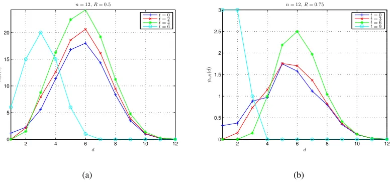
The second experiment studies the effect of tail length t on the HDS of DA codes. Some examples are given in Fig. 3, where code length n = 12. The results in Fig. 3 are obtained by (32) with refinedψn,R(n)using (37). In Fig. 3(a), we setR = 0.5and thust∈[0 :nR] = [0 : 6].

In Fig. 3(b), we set R= 0.75 and thus t∈[0 :nR] = [0 : 9]. It can be seen that, as t increases (not very near to bitstream length nR), ψn,R(d) will tend to be smaller (and even become 0 in

some cases) for small d but tend to be larger for large d. Note that the HDS when t =nR is very different from the HDS’s in other cases. Thus, the correctness of (44) is verified.

C. Closely-Spaced Fellow Codewords

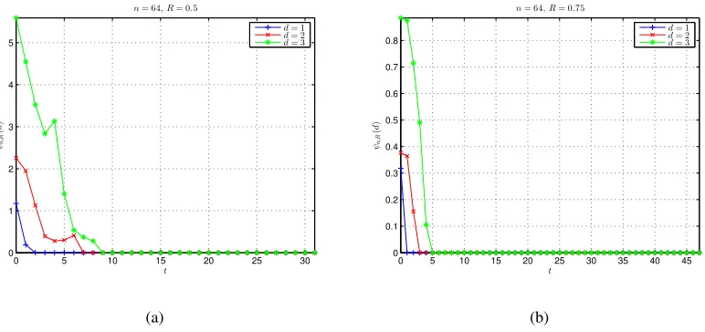
The third experiment studies the effect of tail length t onψn,R(d) for small d. Two examples

0 5 10 15 20 25 30 0

1 2 3 4 5

t ψn,R

(

d

)

n= 64,R= 0.5

d= 1

d= 2

d= 3

(a)

0 5 10 15 20 25 30 35 40 45

0 0.1 0.2 0.3 0.4 0.5 0.6 0.7 0.8

t ψn,R

(

d

)

n= 64,R= 0.75

d= 1

d= 2

d= 3

(b)

Fig. 4. Effect of tail length on ψn,R(d) for small d, where n = 64. The results are obtained by (32). (a) R = 0.5. (b)

R= 0.75.

4 are obtained by (32). It can be seen that in general, ψn,R(d) for small d tends to be smaller

as t increases, implying that closely-spaced fellow codewords can be removed by increasing tail length t (not very near to bitstream length nR). However, it must be pointed out that the decrease of ψn,R(d) for small d w.r.t. t is not strictly monotonous, so tail length t should be

carefully chosen in practice to optimize the overall performance.

D. Average Codebook Cardinality and Rate Loss

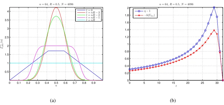
The last experiment studies the effect of tail length t on the ACC and rate loss of DA codes. Since both ACC and rate loss are closely related to the initial CCS, some examples of f_n,R,t(0) (u)

are given in Fig. 5(a), where n = 64 and R = 0.5. By comparing the curve of t = 0 with the curve of t= (nR−3), it can be seen that for t not very close to nR, f_n,R,t(0) (u) does tend to be spikier as t increases. However, as t approaches nR, there is an opposite trend, i.e., f_n,R,t(0) (u)

tends to be flatter. In the extreme case of t=nR, f_n,R,t(0) (u) is uniform over [0,1).

Correspondingly, some examples of(η−1)and−h(U0,n)versustare given in Fig. 5(b), where

n= 64 andR = 0.5. Note thatηand−h(U0,n)are obtained by (84) and (85), respectively. It can

be seen that, for t not very near tonR, both η and −h(U0,n) will go up ast increases, meaning

0 0.1 0.2 0.3 0.4 0.5 0.6 0.7 0.8 0.9 0.5

1 1.5 2 2.5 3 3.5 4

u

f

(0

)

n

,R

,t

(

u

)

n= 64,R= 0.5,N= 4096

t= 0 t=nR−3 t=nR−2 t=nR−1 t=nR

(a)

0 5 10 15 20 25 30

0 0.2 0.4 0.6 0.8 1 1.2 1.4 1.6 1.8 2

t

n= 64,R= 0.5,N= 4096

η−1

−h(U0,n)

(b)

Fig. 5. Examples of initial CCS, ACC scaling factor, and rate loss of DA codes, weren= 64andR= 0.5. The results are obtained by the numerical algorithm given in Sect. VIII with cell numberN = 4096. (a) Initial CCS of DA codes versus tail length. (b) ACC scaling factor and rate loss of DA codes versus tail length.

the extreme case of t =nR, η = 1 and −h(U0,n) = 0. The reason is: When t = nR, Xn(1−R)

is not transmitted, while X_nn_(1−R) is transmitted in its uncoded form, so there is no rate loss for uniform binary sources. However, as shown by (44) and Fig. 3, the HDS is indeed a binomial function when t=nR, so DAC’s performance is very poor in this case.

X. CONCLUSION

This paper discusses the effect of tail length on DA codes from two aspects: HDS and CCS. Both exact and approximate HDS formulas are derived for tailless DAC and extended to tailed DAC. It is revealed that closely-spaced fellow codewords can be removed by increasing tail length to a value not near to bitstream length, which explains the superiority of tailed DAC over tailless DAC. On the basis of CCS, the ACC and rate loss of tailed DAC are derived and it is shown that increasing tail length to a value not near to bitstream length will raise decoding complexity and rate loss. These findings indicate that increasing tail length will usually bring both positive (removing closely-spaced fellow codewords) and negative (raising decoding complexity and rate loss) effects, so tail length should be selected carefully to optimize the overall performance. However, it is also found that the effects of tail length are sometimes surprising, e.g., ψn,R(d)

REFERENCES

[1] J. Rissanen, “Generalized Kraft inequality and arithmetic coding,” IBM J. Research & Development, vol. 20, no. 3, pp. 198–203, May 1976.

[2] I. Witten, R. Neal, and J. Cleary, “Arithmetic coding for data compression,” Commun. of the ACM, vol. 30, no. 6, pp. 520–540, Jun. 1987.

[3] M. Grangetto, E. Magli, and G. Olmo, “Distributed arithmetic coding,”IEEE Commun. Lett., vol. 11, no. 11, pp. 883–885, Nov. 2007.

[4] M. Grangetto, E. Magli, and G. Olmo, “Distributed arithmetic coding for the Slepian-Wolf problem,” IEEE Trans. Signal Process., vol. 57, no. 6, pp. 2245–2257, Jun. 2009.

[5] D. Slepian and J. Wolf, “Noiseless coding of correlated information sources,” IEEE Trans. Inform. Theory, vol. 19, no. 4, pp. 471–480, Jul. 1973.

[6] J. Garcia-Frias and Y. Zhao, “Compression of correlated binary sources using turbo codes,” IEEE Commun. Lett., vol. 5, no. 10, pp. 417–419, Oct. 2001.

[7] A. Liveris, Z. Xiong, and C. Georghiades, “Compression of binary sources with side information at the decoder using LDPC codes,” IEEE Commun. Lett., vol. 6, no. 10, pp. 440–442, Oct. 2002.

[8] M. Grangetto, E. Magli, and G. Olmo, “Security applications of distributed arithmetic coding,” in:Proc. 18th European Signal Process. Conf. (EUSIPCO-2010), pp.2151–2155, Aalborg, Denmark, Aug. 23–27, 2010.

[9] X. Artigas, S. Malinowski, C. Guillemot, and L. Torres, “Overlapped quasi-arithmetic codes for distributed video coding,” in:Proc. IEEE ICIP, 2007, vol. II, pp. 9–12.

[10] S. Malinowski, X. Artigas, C. Guillemot, and L. Torres, “Distributed coding using punctured quasi-arithmetic codes for memory and memoryless sources,” IEEE Trans. Signal Process., vol. 57, no. 10, pp. 4154–4158, Oct. 2009.

[11] X. Chen and D. Taubman, “Distributed source coding based on punctured conditional arithmetic codes,” in:Proc. IEEE ICIP, pp. 3713–3716, Sep. 2010.

[12] X. Chen and D. Taubman, “Coupled distributed arithmetic coding,” in:Proc. IEEE ICIP, pp. 341–344, Sep. 2011. [13] J. Zhou, K. Wong, and J. Chen, “Distributed block arithmetic coding for equiprobable sources,” IEEE Sensors Journal,

vol. 13, no. 7, pp. 2750–2756, Jul. 2013.

[14] M. Grangetto, E. Magli, R. Tron, and G. Olmo, “Rate-compatible distributed arithmetic coding,”IEEE Commun. Lett., vol. 12, no. 8, pp. 575–577, Aug. 2008.

[15] M. Grangetto, E. Magli, and G. Olmo, “Distributed joint source-channel arithmetic coding,” in:Proc. IEEE Int’l Conf. Image Process. (ICIP), 2010, pp. 3717–3720.

[16] Y. Keshtkarjahromi, M. Valipour, and F. Lahouti, “Multi-level distributed arithmetic coding with nested lattice quantization,” in:Proc. IEEE Data Compression Conference (DCC), pp. 382–391, Mar. 26–28, 2014.

[17] Z. Wang, Y. Mao, and I. Kiringa, “Non-binary distributed arithmetic coding,” in:Proc. IEEE 14th Canadian Workshop Inform. Theory (CWIT), pp. 5–8, Jul. 2015.

[18] Y. Fang, “DAC spectrum of binary sources with equally-likely symbols,” IEEE Trans. Commun., vol. 61, no. 4, pp. 1584–1594, Apr. 2013.

[19] Y. Fang and L. Chen, “Improved binary DAC codec with spectrum for equiprobable sources,”IEEE Trans. Commun., vol. 62, no. 1, pp. 256–268, Jan. 2014.