This is a repository copy of
Spatio-temporal generalised frequency response functions
over bounded spatial domains
.
White Rose Research Online URL for this paper:
http://eprints.whiterose.ac.uk/74669/
Monograph:
Guo, L.Z., Guo, Y.Z., Billings, S.A. et al. (2 more authors) (2010) Spatio-temporal
generalised frequency response functions over bounded spatial domains. Research
Report. ACSE Research Report no. 1018 . Automatic Control and Systems Engineering,
University of Sheffield
[email protected] https://eprints.whiterose.ac.uk/
Reuse
Unless indicated otherwise, fulltext items are protected by copyright with all rights reserved. The copyright exception in section 29 of the Copyright, Designs and Patents Act 1988 allows the making of a single copy solely for the purpose of non-commercial research or private study within the limits of fair dealing. The publisher or other rights-holder may allow further reproduction and re-use of this version - refer to the White Rose Research Online record for this item. Where records identify the publisher as the copyright holder, users can verify any specific terms of use on the publisher’s website.
Takedown
If you consider content in White Rose Research Online to be in breach of UK law, please notify us by
Spatio-temporal Generalised Frequency
Response Functions over Bounded Spatial
Domains
L. Z. Guo, Y. Z. Guo, S. A. Billings, D. Coca, Z. Q. Lang
Research Report No. 1018
Department of Automatic Control and Systems Engineering
The University of Sheffield
Mappin Street, Sheffield,
S1 3JD, UK
Abstract—In a companion paper (Guo, Guo, Billings, Coca, and Lang 2010), the concept of frequency response functions (GFRFs) has been extended to describe the characteristics of spatio-temporal dynamical systems over an unbounded spatial domain from a frequency domain point of view. In this paper, a similar point of view will be taken to investigate spatial-temporal dynamical systems over a bounded spatial domain in the frequency domain. The main difference is that due to the bounded spatial domain, the property of translation invariance with respect to the spatial domain is not valid any more. In order to overcome this, the paper provides a new definition of impulse response functions, which is different from the standard impulse definitions. The definitions and interpretation of spatio-temporal generalised frequency response functions are given for linear and nonlinear spatio-temporal systems based on this newly defined impulse response function. Examples are provided to illustrate the new frequency domain methods.
Index Terms—Generalised frequency response, spatio-temporal systems, bounded spatial domain, Volterra series representation
I. INTRODUCTION
In a companion paper (Guo, Guo, Billings, Coca, and Lang 2010), it has been shown that the concept of generalised frequency response functions (GFRFs) can be extended to describe the characteristics of spatio-temporal dynamical systems over an unbounded spatial domain from a frequency domain point of view. Generalised impulse response functions, generalised transfer functions, and generalised frequency response functions can be defined for linear/nonlinear spatio-temporal systems over an unbounded spatial domain, which are consistent with their traditional meanings. The reason why this could be done is that the underlying system is both time and spatial translation invariant, which requires the spatial domain is infinite/unbounded. With these properties, the impulse response functions can be defined properly and the Laplace or Fourier transformations can be applied without any difficulties.
This naturally leads to the definition of transfer functions or frequency response functions for spatio-temporal systems over an unbounded spatial domain. Similar ideas can also be found in Dudgeon and Mersereau (1984). However, this approach cannot be used to do the frequency analysis for spatio-temporal dynamical systems over a finite/bounded spatial domain.
As discussed in Guo, Guo, Billings, Coca, and Lang (2010), a number of different descriptions of the transfer function and frequency response models for spatio-temporal systems, which can deal with a finite/bounded spatial domain have been proposed including Curtain and Zwart (1995), Curtain and Morris (2009), Rabenstein and Trautmann (2002), Garcia-Sanz, Huarte, and Asenjo (2007), Billings and Wei (2007), but most of them are only suitable for linear spatio-temporal systems rather than nonlinear systems. In this paper, motivated by Zadeh (1950), the transfer functions and frequency response approaches are developed and extended to deal with nonlinear spatio-temporal systems over a bounded spatial domain. This is achieved by adopting a new definition of the (generalised) impulse response functions of the system with respect to an excitation signal through external inputs, initial conditions or boundaries. This definition of the impulse response functions is different from the traditional methods in the sense that it indicates the position where the impulse signal is applied explicitly. It allows us to deal with the bounded spatial domain in an effective way and leads to the definition of (generalised) frequency response functions in a natural way. The paper is organised as follows. An analysis of the impulse and frequency responses for linear spatio-temporal systems over bounded spatial domain is given in Section 2, which includes three different types of impulse response and frequency response functions and how to calculate them. The formal definitions of the GTFs and GFRFs for nonlinear spatio-temporal systems over a finite spatial domain are then given in Section 3, together with a detailed analysis of these functions. Section 4 illustrates the proposed methods using some numerical examples of linear and nonlinear spatio-temporal systems. Conclusions are drawn in Section 5.
Spatio-temporal Generalised Frequency
Response Functions over Bounded Spatial
Domains
L. Z. Guo, Y. Z. Guo, S. A. Billings, D. Coca, and Z. Q. Lang
II. SPECTRAL ANALYSIS OF LINEAR SPATIO-TEMPORAL SYSTEMS
In this section, we will consider linear, time-invariant spatio-temporal systems governed by the following first order evolution equation
(1)
where is the space coordinate variable defined on a bounded domain with a boundary and is the time variable. A is a bounded linear operator which can, for example, take the form of
, where , , and represent the temporal derivative, first and second order spatial derivatives, respectively. and are the linear operators for defining the initial and boundary conditions. We assume that and denote the output and the external excitation of the system, respectively. For simplicity, in this initial study, we restrict our discussion to one spatial dimension and scalar systems, which gives . In this case, certain boundary conditions are required to obtain a unique solution to (1). The general form of the boundary conditions is
(2)
which includes four commonly used boundary conditions: Dirichlet ( ),
Newmann ( ), Robin
( ), ,
and periodic ( )). The initial-boundary value problem is then given as
(3)
which can be split into four sub-problems
homogeneous equation with zero initial conditions and inhomogeneous boundary conditions at a
(4)
homogeneous equation with zero initial conditions and inhomogeneous boundary conditions at b
(5)
homogeneous equation with nonzero initial conditions and homogeneous boundary conditions
(6)
Inhomogeneous equation with zero initial conditions and homogeneous boundary conditions
(7) If , , ,and are the solutions to (4)-(7), then superposition shows that the solution to (3) is the sum of these four solutions due to the linearity. The problem here is to derive the impulse response functions and frequency response functions of the system (3) over . In what follows, we will discuss them separately.
A. Impulse and Frequency Responses With Respect To Boundary Conditions
The impulse and frequency responses with respect to boundary conditions are related to problem (4) and (5). In this section, we will discuss problem (4) while (5) can be treated in a similar manner. Setting
in (4) gives a solution to (4) as
(8) It follows that given a general boundary condition and considering the time-invariance, the solution to (4) will be
(9) which means the solution to (4) is the convolution of and with respect to time. The function is obviously the system response at time caused by an impulse applied at time and at boundary point . Therefore, it will be referred to as the impulse response function of the system (3) with respect to boundary conditions.
(10) Substituting (10) into (9) gives
(11)
which shows that the output is a scaled version of the input , which means is the eigenfunction of (4) with eigenvalue . Therefore, it is natural to define
(12) as the frequency response of the system (3) with respect to its boundary conditions.
It is also interesting to notice that as a function of spatial variable , may be expanded in a Fourier series as a periodic function with a period of
(13) where
(14)
B. Impulse and Frequency Responses With Respect To Initial Conditions
To derive the impulse and frequency responses with respect to initial conditions, consider (6) with an impulse initial condition
(15) Denote the solution to (15), and then for a general initial condition , the solution to (6) is given by
(16) Notice that is a spatial position where the impulse is applied. Let be the relative position of with reference to position . A change of variable in (16) results in
(17)
where . The
function may be interpreted as the response of the system (3) at time and spatial location caused by an impulse applied spatial locations with reference to the site at time . We will define this function as the impulse response of the system (3) with respect to initial conditions, which depends on spatial location.
The impulse function
has a Fourier series expansion considered as a periodic function of
as follows
(18) where
(19) If the function is of the following form
(20) which can be considered as being defined over or a periodic extension, substituting (20) into (17) yields
(21)
which shows that is the eigenfunction of (6) with eigenvalue . Therefore, it is natural to define
(22) as the frequency response of the system (3) with respect to its initial condition, which is the ratio of the system output to the harmonic initial excitation.
C. Impulse and Frequency Responses With Respect To External Excitations
argument in previous sections. Now consider the problem (7) with an impulse excitation
(23) Denote the solution to (23), then for a general external excitation , the solution to (7) will be
(24) due to the assumption of time-invariance. As for the spatial variable, again let be the relative position of with reference to position and a change of variable in (24) results in
(25)
where . We will
define this function as the impulse response of the system (3) with respect to external excitation, which depends on spatial location due to the loss of spatial invariance.
If the external excitation is of the following form
(26) substituting (26) into (25) yields
(27)
where
(28)
From (28), it can be observed that are the Fourier coefficients of the Fourier series expansion of the function
(29) Therefore, from (27) one has
(30) We will call the frequency response function of the system (3) with respect to external excitation.
D. Computation of the Linear Frequency Response Functions
In this section a simple example will be used to show how to calculate the frequency response functions discussed in previous sections.
Consider a linear system described by the following first order evolution equation with a Neumann boundary condition
(31) where are constants. The frequency response functions to be calculated are ,
, and .
To calculate , suppose , from (11) the output and the associated temporal and spatial derivatives are then
(32) Substituting equation (32) and into equation (31) with yields
(34) with the following characteristic equation
(35) To calculate , suppose , from (21) the output and the associated temporal and spatial derivatives are then
(36) Substituting equation (36) and into equation (31) with yields
(37) The frequency response function can be obtained as the solution to the initial boundary value problem (37).
To calculate , assume the input to (21) is , from (27) the output and the associated temporal and spatial derivatives are then
(38) Substituting equation (38) and
into equation (31) with yields
(39) The frequency response function can be obtained as the solution to the boundary value problem (39) with a characteristic equation
(40)
III. SPECTRAL ANALYSIS OF
NONLINEAR SPATIO-TEMPORAL SYSTEMS
In this section, we extend the idea of impulse response functions and frequency response functions for linear spatio-temporal systems over a bounded spatial domain to the nonlinear cases using a Volterra series representation of the nonlinear relationships.
Consider the following first order nonlinear evolution equation with initial conditions I and boundary conditions B
(41) where A is a bounded nonlinear operator which can, for example, take a form of . As in the linear case, define and to be the output and the external excitation of the system, respectively. Similar to the linear case, we will also investigate the impulse responses of the following equations derived from equation (41)
homogeneous equation with zero initial conditions and inhomogeneous boundary conditions at a
(42)
homogeneous equation with zero initial conditions and inhomogeneous boundary conditions at b
(43)
homogeneous equation with nonzero initial conditions and homogeneous boundary conditions
Inhomogeneous equation with zero initial conditions and homogeneous boundary conditions
(45) Remark 1. Due to the nonlinearity of the operators involved, the solutions , of (42), (43), (44), and (45) may not be expressed according to the linear convolution between the impulse response functions and the inputs because there are nonlinear (dynamical) relations between the input and output. In this paper, we will use a Volterra series representation to describe these nonlinear relationships.
Following the general nonlinear system and Volterra series representation theory (Schetzen 1980, Rugh 1981), the four solutions can be expressed as the Volterra series representations
(46) where , , , and are the nth order outputs of the system with
(47) Define the functions , , and and as the nth order generalised impulse response functions of the system with respect to external signals, initial conditions, and boundary conditions, respectively. In this paper, it is assumed that the generalised impulse functions are symmetric with respect to all the time and all the spatial variables. In what follows we will derive the generalised frequency response functions for each of them.
Remark 2. The first two Volterra series
representations in (46) and (47) come from the assumption that the system (41) is time-invariant while the last two representations follow the same approach as discussed in the previous section. Because the spatial domain is bounded, the system (41) is not spatially translation invariant or is not stationary so that we again use relative locations
instead of the absolute locations for the impulse inputs as discussed in sections II.B and II.C.
Remark 3. Note that in general the solution of (41) may not be the sum of the four solutions in (46) because the operators A, I, and B are nonlinear. This solution could take the following general form
(48)
with ,
where is a nonlinear map.
A. Generalised Frequency Responses With Respect To Boundary Conditions
If the function is of the following form
(49) Substituting (49) into the first equation of (47) gives (due to the assumption of symmetry)
(50) Where
(51) We will call the nth generalised frequency response function of the nonlinear spatio-temporal system (41) with respect to boundary conditions. can be defined following a similar argument.
B. Generalised Frequency Responses With Respect To Initial Conditions
For the sake of simplicity, it will be assumed that so that the spatial domain is . If the function is of the following form
(52) which can be considered as being defined over or a periodic extension, substituting (52) into the third equation in (47) yields
(53) Where
(54) Therefore, in (54) can be understood as the coefficients of the multidimensional Fourier series representation of the impulse response function
(55) We will call the nth generalised frequency response function of the nonlinear spatio-temporal system (41) with respect to initial conditions.
C. Generalised Frequency Responses With Respect To External Excitation
Again if it is assumed that so that the spatial domain is . If the function is of the following form
(57) where
(58) If we let
(59) in (58) can be understood as the coefficients of the multidimensional Fourier series representation of the function in (59)
(60) We will call the nth generalised frequency response function of the nonlinear spatio-temporal system (41) with respect to external excitation. can be considered to be obtained from Fourier transform for the time variable and then Fourier series expansion for the spatial variable.
D. The Calculation of Spatio-temporal Generalised Frequency Response Functions
Consider an example nonlinear system described by the following first order evolution equation with Dirichlet boundary condition
(61)
where are constants. The frequency response functions to be calculated are ,
, and ,
corresponding to the problems (43), (44), and (45). The calculation of these nth spatio-temporal generalised transfer functions can be carried out using a development of the probing method (Billings and Tsang 1989a, Peyton-Jones and Billings 1989, Billings and Peyton-Jones 1990, Bedrosian and Rice 1971).
To calculate suppose and from (50)
(62) Substituting equation (62) and into equation (61) with , and equating the coefficients of the term yields
(63) The first order generalised frequency response function can then be obtained as the solution to the boundary value problem (63).
To calculate , suppose the input is , again from (50)
(64) Substituting (64) and the associated temporal derivative and spatial derivatives , and equating the coefficients of the term yields
(65) It follows that is the solution to the boundary value problems (65).
(66) Inserting (66) into (61) with and equating the coefficients of the term yields
(67) The solution to the initial-boundary value problem (67) is the required first order generalised frequency response function . The second order frequency response function can be obtained by using
as test signal, where is the magnitude. Now from the definition (47), the respective components of the response are then
(68) and
(69) Without loss of generality, it is assumed that
are positive integers. Substituting (69) with (68) and its associated derivatives and equating coefficients of the
term gives
(70) It follows that the second order generalised frequency response function will be the solution to the initial-boundary value problem (70).
The other order spatio-temporal generalised frequency response functions can be calculated following a similar procedure.
IV. NUMERICAL EXAMPLES
A. Linear Spatio-temporal Systems -- Diffusion Equation
Consider the following diffusion equation (Debnath 2005) with Dirichlet boundary conditions
(71) where D is the positive diffusion coefficient. According to the analysis in section 2, system (71) can be divided into three subsystems with the corresponding frequency response functions , , and
.
To calculate the boundary frequency response , suppose an input of , then
(72) whose solution is given by
[image:11.612.70.285.314.620.2]the result of example 1 discussed in Curtain and Morris (2009) is a special case of the result here.
The frequency response is related to the following problem
(74) For simplicity, we set . Suppose the input to (74) is , the output and the associated temporal and spatial derivatives are then
(75) Substituting (75) and into equation (74) yields
(76) The initial-boundary value problem (76) can be solved by separation of variables, whose solution is
(77) where satisfy
(78) is the Kronecker delta.
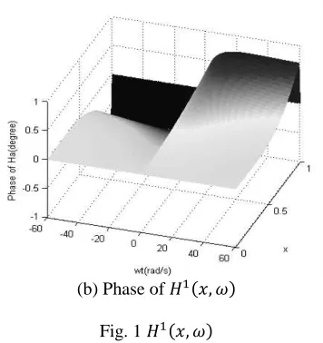
(a) Magnitude of
[image:12.612.346.524.75.264.2](b) Phase of
Fig. 1
To calculate the frequency response with respect to the external excitation, we consider the problem
(79) Again we set to simplify the computation. Suppose the input to (79) is
, the output and the associated temporal and spatial derivatives are then
(80) Substituting (80) and into equation (79) yields
(81) The solution to the boundary value problem (81) is the required frequency response function
(82) where
(83)
B. Nonlinear Spatio-temporal Systems
Consider again the nonlinear system (61) described in section III.D with parameters , and
, which is
(84) We are going to calculate the first and second order generalised frequency response functions
and .
To calculate , suppose the input to (84) is , then the output and the associated temporal and spatial derivatives are
(85) Substituting equation (85) and
into equation (84) and equating the coefficients of the term yields
(86) The solution to (86) is the required frequency response function
(87) where
(88) To calculate , suppose the input
is ,
. Following the earlier discussion, the response is then
(89) Substituting (89) and the associated temporal derivative and spatial derivatives , and equating the coefficients of the term
yields
(90) The characteristic equation of (90) is
(91)
V. CONCLUSIONS
computation of these functions and their interpretations are necessary.
ACKNOWLEDGEMENTS
The authors gratefully acknowledge support from the UK Engineering and Physical Sciences Research Council (EPSRC) and the European Research Council (ERC).
REFERENCES
Bedrosian, E. and Rice, S. O. (1971), The output properties of Volterra systems (nonlinear systems with memory) driven by harmonic and Gaussian inputs, Proceedings IEEE, Vol. 59, pp. 1688-1707.
Billings, S. A. and Wei, H. L. (2007), Characterising linear spatio-temporal dynamical systems in the frequency domain, Research Report 944, The University of Sheffield.
Billings, S. A. and Peyton-Jones, J. C. (1990), Mapping nonlinear integro-differential equations into the frequency domain, Int. J. Cont, Vol.52, pp. 863-879.
Billings, S. A. and Tsang, K. M. (1989a), Spectral analysis for non-linear systems, Part I: parametric non-linear spectral analysis, Mechanical Systems and Signal Processing, Vol.3, No.4, pp. 319-339. Billings, S. A. and Tsang, K. M. (1989b), Spectral analysis for non-linear systems, Part II: Interpretation of non-linear frequency response functions, Mechanical Systems and Signal Processing, Vol.3, No.4, pp. 341-359.
Curtain, R. F., and Morris, K. (2009), Transfer functions of distributed parameter systems: A tutorial, Automatica, Vol, 45, pp. 1101-1116.
Curtain, R. F., and Zwart, H. J. (1995), An Introduction to Infinite-Dimensional Linear Systems theory, New York: Springer-Verlag.
Debnath, L. (2005), Nonlinear partial differential equations for scientists and engineers (2nd ed.), Boston: Birkhauser.
Dudgeon, D. E., and Mersereau, R. M. (1984), Multidimensional digital signal processing, New Jersey: Prentice-Hall.
Garcia-Sanz, M., Huarte, A., and Asenjo, A. (2007), A quantitative robust control approach for distributed parameter systems, Int. J. Robust Nonlinear Control, Vol. 17, pp. 135–153.
Guo, L. Z., Guo, Y. Z., Billings, S. A., Coca, D., and Lang, Z. Q. (2010), Spatio-temporal generalised frequency response functions over unbounded spatial domain, Research Report, The University of Sheffield.
Marmarelis, P. Z. and Marmarelis, V. Z. (1978), Analysis of Physiological Systems – the White Noise Approach, New York: Plenum Press.
Peyton-Jones, J. C. and Billings, S. A. (1989), A recursive algorithm for computing the frequency response of a class of nonlinear difference equation model, Int. J. Cont, Vol.50, pp. 1925-1940.
Rabenstein, R. and Trautmann, L. (2002), Multidimensional transfer function models, IEEE Trans. Circu. & Syst.- Fundamental Theory and Application, Vol. 49, No.6, pp. 852-861.
Rugh, W. J. (1981), Nonlinear System Theory – The Volterra/Wiener Approach, London: The Johns Hopkins University Press.
Schetzen, M. (1980), The Volterra and Wiener Theories of Nonlinear systems, Chichester: John Wiley.