Tomography
Inside yourself or outside, you never have to change what you see, only the way you see it.
– Thaddeus Golas
F
or many years, the challenge of determining the internal structure of an object—while not actually damaging the object itself—has attracted great in-terest. From the Greek word tomos meaning ’slice’ or ’section’, tomography seeks to recover the internal structure based on line-of-sight measurements of some quantity or property of the object. Figure 3.1 illustrates this concept. The the-ory of tomography is based on the work of Radon [Radon, 1917] which ob-tains an analytic formula for the inversion of the line-integral, or ‘Radon’ trans-form. An application for which tomography is perhaps most widely known is its use in medical imaging, where it is known as CT (computed tomography) or CAT scanning. Pioneering work by Hounsfield [Hounsfield, 1973], and Cor-mack [CorCor-mack, 1963], [CorCor-mack, 1964] was recognised with their joint award of the Nobel Prize in Physiology or Medicine in 1979 “for the development of computer assisted tomography”. Other applications are many and varied and include include earlier work in radio astronomy [Bracewell, 1956a], [Bracewell, 1956b], more medical imaging [Mazziotta et al., 1986] including magnetic reso-nance imaging (MRI) [Damadian, 1971], [Lauterbur, 1973]†, supersonic gas flows [Morton, 1995] and seismology [Nolet, 1987].The line-integrated measurements of the object under investigation can be obtained, depending on the nature of the object, by many varied techniques. The challenge is to invert the profiles created by the line-integrated measurements to give the correct, or at least the best approximation of, the internal structure of the object. This chapter outlines the theory for the tomographic inversion techniques used in this thesis, as well as considerations regarding their use.
Simulations demonstrating the performance of these procedures—applied with the experimental configuration used in this thesis—are also presented.
p y(p,
φ)
φ
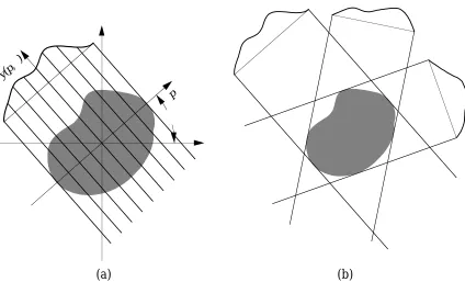
[image:2.595.119.543.94.351.2](a) (b)
Figure 3.1: (a) Line integrals are used to construct a profile of an object. (b) Several profiles are used to build a cross-section of the object. Figure courtesy of G. Warr.
3.1 Theory
For two-dimensional tomography, the object or picture from which the line-integrated measurements are obtained can be represented by a function of two variables. This is known as the picture function, denoted as P(r)and is defined to be zero outside the picture region.
The Radon transform of the picture function is defined as
ˇ
P =RP =
L
P(r)dl (3.1)
where dl is the element along the line L and the symbols and geometry are given in Figure 2.1.
In a typical experimental situation, P(r)might represent the emissivity in the (x, y)plane, L the line of sight and ˇP the measurement along that line.
It is convenient to re-write the Radon transform of (3.1) in terms of the impact parameter p and angleφas
ˇ
P(p,φ) =
P(r)δ(p− ˆp.r)dr (3.2)
where the Dirac delta functionδis used to select the line L.
reconstruction technique (ART) and linear composition of orthogonal functions, both of which are utilised in this thesis. The other approach using Fourier and Hilbert transform methods is not discussed here.
For the ith line-integrated measurement yi—associated with the line of sight
specified by(pi,φi)and with a total of I measurements—the Radon transform of
P for this line is
yi =RiP (3.3)
and Ri is a functional. That is, it acts on a function to produce a real number. A collection of line integrals associated with a specific viewing position of the object is known as a projection. Figure 3.1(a) shows a simple arrangement for a projection using parallel lines with a constantφi. The entire set of measurements
y is known as the measurement vector and it is assumed that the set of lines is fixed and known.
The input data for the reconstructions are then samples of the Radon trans-form and the reconstruction itself becomes an approximation of the picture func-tion. This approximation can be made arbitrarily good by utilising an increasing number of projections [Hamaker et al., 1980]. For a finite set however, a theorem [Smith et al., 1977] states: A function P of compact support in R2is uniquely de-termined by any infinite set, but by no finite set of its projections. Even though uniqueness is sacrificed in real applications, the challenge is to closely approxi-mate the real P with non-unique approximations. This can be done using a priori information, knowledge before the fact, to help define the solution.
The series expansion methods discretise the picture function into basis pic-tures. A basis picture may represent, among other things, a spatial area (a ‘tra-ditional’ pixel) or a function. The estimate of the picture function is given by a linear combination of the basis pictures. If the jth basis picture is denoted as bj, with a total of J basis pictures, then the picture function estimate can be written as
P(r) =
∑
j
xjbj (3.4)
where xj is the value (a co-efficient or weighting) for the basis picture and the
complete set x is known as the image vector. Substituting (3.4) into (3.3) gives
yi
∑
j
Rijxj (3.5)
where Rij Ribj. The matrix R, whose (i, j) element is Rij, is known as the response or projection matrix. The difference between the left and right hand sides of (3.5) is given as eiand the aim of the reconstruction of the picture function
estimate is to minimise this error vector. Allowing for this discrepancy, (3.5) is more succinctly written, in matrix form, as
The difference vector e may be due to errors in the measurements or an inability to adequately describe the picture function.
3.2 Methods of Reconstruction
3.2.1 Algebraic Reconstruction Techniques
These methods, often abbreviated as ART, were first proposed by [Gordon et al., 1970] and [Hounsfield, 1972] and though not actually any more algebraic than other series expansion methods—the name is a historical accident—they are iterative in nature. A sequence of image vectors x(0), x(1), x(2), ... converge to a final estimate image vector x∗. x(k+1) is derived from x(k)based on the relation in (3.5) and the iterative step can be written as a functionαk such that
x(k+1) = αk(x(k), Rik, yik) (3.7)
with a total of K iterations. Here ik is used to denote (k mod I) +1† such that the equations are used cyclically and Ri is the transpose of the ithrow of R. ART methods differ from each other in the choice of the iterative step functionαk.
The ART method primarily employed in this thesis uses an iterative-step function of the form
αk = x(k)+
σ(yik−∑jRikjx(jk))
J (3.8)
where σ is a relaxation factor to allow the solution to converge in a controlled way. This iterative-step function adds to the image vector a mean of the differ-ence between the measurement data and the response matrix-weighted sum of the current image vector†, modified by the relaxation factor. Other constraints may be imposed on the iterative step function such as ensuring the right-hand side of (3.8) is positive or smoothing the image vector between iterations. In prac-tice, the computation is restricted to basis pictures which are directly associated with a given line-integrated measurement.
3.2.2 Linear Composition of Orthonormal Basis Functions
Recalling that the definition of a ‘basis picture’ (§3.1) equally refers to a func-tion as it does to a spatial area, this reconstrucfunc-tion method builds the picture function as a linear composition of carefully chosen basis functions. Some a priori information about the general structure of the object is required so that a suitable
†That is, i
0=1, i1=2, ..., iI−1=I, iI =1, iI+1=2, ...
family of functions may be selected. If the magnetic field structure is transformed to flux co-ordinates—where the nested flux surfaces become simple circles and the outermost has a radius of unity—a combination of radial and angular func-tions may be used to describe the picture function. Working in flux co-ordinates has the additional advantage of being able to use any symmetry arguments, such as constancy on a flux surface, which may help to further constrain the recon-struction.
The original Cormack inversion used Zernicke polynomials in the radial co-ordinate and Fourier functions in the angular co-co-ordinate. However for picture functions which are zero at their boundary a more suitable choice for the radial component is Bessel functions [Nagayama, 1987].
For flux co-ordinates(r,θ), the Fourier-Bessel function is given as [Warr, 1998]
Fml(r,θ) =
√
2
|Jm (ml)|Jm(mlr)e
imθ (3.9)
where ml are the roots of the Bessel functions (Jm(ml) = 0) and scale r so that
Jm(mlr)is zero at r = 1. Jm = drd Jm is the derivative and the normalising factor
√
2/|Jm (ml)|ensures orthonormality. The picture function is then given by
P(r,θ) =
L
∑
0 M∑
−MχmlFml(r,θ) (3.10)
where χml is a complex co-efficient and the total number of functions used is given by
J = (2M+1)(L+1) (3.11)
If the object is real, the co-efficients must satisfy the Hermitian symmetry
χml =χ∗ml (3.12)
To determine the vector of co-efficientsχ, (3.6) is re-written as
χ = R−1(y−e) (3.13)
However since R is often ill-conditioned, singular value decomposition (SVD) [Press et al., 1986, pages 52–64]† is used to find the inverse which may be re-garded, in some sense, as the ‘best’ inverse. If R is an I × J matrix, it can be
decomposed into the product of an I×J column-orthogonal matrix U, a J ×J
diagonal matrix W with elements wj ≥0 and the transpose of a J×J orthogonal
matrix V,
R=UWVT. (3.14)
†This reference contains a more comprehensive treatment of this method than the very brief
Since U and V are orthogonal matrices, the inverse of R is given simply by
R−1 =VW−1UT, (3.15)
where W−1 =diag(1/wj).
The condition number C of the response matrix is obtained while using the SVD method and is a measure of the robustness of the inversion against noise. It is defined as
C = max(wj)
min(wj) (3.16)
The lower the condition number of a given response matrix the more reliable is its inverse. To improve the SVD solution, the wjbelow a certain threshold can be set to zero. In this case min(wj)refers to non-zero values.
Aikake Information Criterion
Since the number of basis pictures (functions) plays an important part in re-covering a reasonable picture function—too many can leave spurious artifacts and too few can fail to describe the function adequately—a useful technique for determining this number is the Aikake Information Criterion (AIC) [Akaike, 1972, 1974]
In the context of this theory it is defined as
AIC= I lne2+2J (3.17)
where . denotes the usual Euclidean vector norm and lower values of AIC indicate a more suitable basis set. The AIC and the condition number of the response matrix are estimators of the overall suitability of a particular set of basis functions.
Coverage in Flux Space
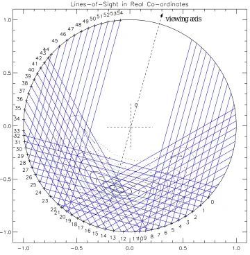
The lines-of-sight (viewing chords) are mapped to flux space via a transform calculated using the GOURDON code. The positions of the viewing chords (pi,φi) in real space for the ToMOSS system are shown in Figure 3.2 and Fig-ure 3.3 shows the coverage in flux space.
Inclusion of the Measured Spatial Response
θ0
[image:7.595.146.506.210.578.2]viewing axis
3.3 Simulations of Emissivity
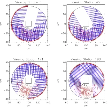
Simulations have been performed to analyse the performance of the ToMOSS system and to verify the tomographic inversion codes. A few of the simulation results are discussed in this section. Using the rotational abilities of the light-collection system, a data set of a few hundred line-integrated measurements can be used to reconstruct the picture function. The light collection system and its capabilities are described in detail in §4.1 and §5.1. Figure 3.4 shows a few of the available viewing stations—a unique configuration of lines-of-sight obtained by rotation of the light-collection optics. The station number represents the angle of anti-clockwise rotation from Viewing Station 0. Test picture functions, including a ‘hat’ function bounded by the last closed flux surface and small width objects at different locations in the viewing region, have been reconstructed using the ART method.
Testing of the Fourier-Bessel basis function method included reconstructing a two-dimensional twin-Gaussian function. The basis function method does not need to rotate the light collection system, but uses data from only a single view-ing station. Though the capacity to use many viewview-ing stations in conjunction with the basis functions method certainly exists, requiring only a single view-ing station allows the system to capture the dynamic behaviour of the plasma without relying on shot-to-shot reproducibility.
3.3.1 ART Tests
Last Closed Flux Surface ‘Hat’ Function
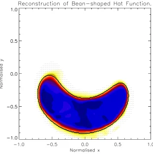
A ‘hat’ function bounded by the last closed flux surface of the standard mag-netic field configuration is reconstructed using the ART method. The function and reconstruction are shown in Figure 3.5). The viewing stations used were 0, 9, 18, 27, 36, 45, 171, 180, 189 and 198 for a total of 460 line-of-sight measure-ments. A normalised, circular convolution kernel was used to smooth the image between iterations. The overlaid points show the effective pixel spacing—the product of the smoothing kernel size and the actual pixel spacing—and the mask used to define pixels involved with the computation. Note that the mask extends beyond the function edge and does not bound the reconstruction. The recon-struction shows good uniformity across the main part of the image, dropping quickly with conformity to the ‘hat’ function boundary.
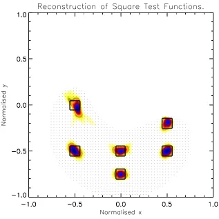
Smaller-Width Square Test Functions
A 3-point convolution kernel was used to smooth the image between iterations. The viewing stations were 0, 9, 18, 27, 36 and 45. The top-left reconstruction is of lower quality than the others due to the limited coverage of viewing chords in that region (see Figure 3.4, top left). Conversely, more line-of-sight measurements to the right side of the viewing region account for the good reconstructions found in this area.
Figure 3.6: A compilation of the ART reconstructions of smaller-width ‘hat’ test func-tions. The original picture function is the overlaid square. The poorer reconstruction at the top-left is due to the lower coverage of lines-of-sight in that region. This can be overcome by rotating the viewing optics a full 180◦from the original viewing station.
3.3.2 Fourier-Bessel Basis Function Test
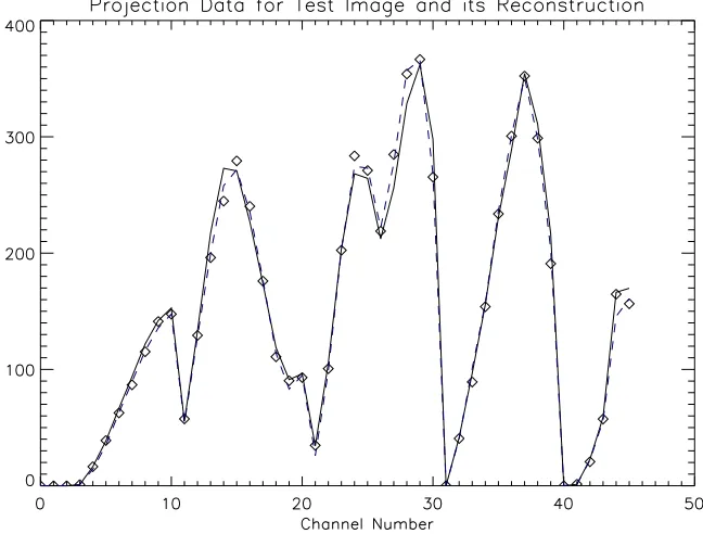
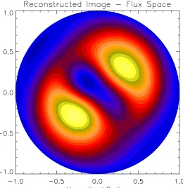
Figure 3.7 shows a function used to test the basis function method—a two-dimensional twin-Gaussian.
The AIC and condition numberC—both shown in Figure 3.9 for different val-ues of M and L—were used to choose the basis function set for the reconstruction.
[image:15.595.124.517.140.448.2]M=2 M=1 M=0
Figure 3.9: The AIC ( ) and the condition numbers of the response matrices (*) for the various mode bases. Degenerate values of a mode basis index are shown in colour. Only response matrices with a condition number of 40 or less are shown.
The mode basis index J (the number of basis functions) is determined by (3.11) and may contain degenerate values. For instance, J =10 for both (M =0, L =9) and(M =2, L= 1). Figure 3.9 indicates that although J =12(M =1, L=3)has a lower condition number for its response matrix, its AIC is considerably higher than J = 15(M = 2, L = 2). Indeed the AIC for J = 18(M = 1, L = 5)is also much higher than for J = 15. A visual inspection of the test function confirms that a basis set that includes only up to M = 1 could not describe it adequately. The next most suitable candidate, according to the AIC, is J =20(M= 2, L=3). Since there is little difference in the AIC (the goodness of fit of the reprojections) for J = 15 and J = 20, the basis set with the lower response matrix condition number is chosen.
3.4 Ion Temperature Tomography
The ToMOSS system is in a unique position to perform tomographic recon-structions of the ion temperature, due to the time-domain nature of the Fourier-encoded interferogram and the good coverage of the plasma region.
The ion temperature Ti is not tomographically inverted in the same way as
emissivity due to the nature of the line-integrated measurement. Recall from (2.24) that Ti is contained in an intensity-weighted measurement of the fringe visibilityζ. The method used in this thesis uses a constrained reconstruction of the image of I0(r)ζ(r)—created via the ART method with spatial basis pictures—
divided by the reconstructed image of I0(r)to give the spatial function of
I0(r)ζ(r)
I0(r) ≡ ζ(r) =exp
−Ti(r) Tc
(3.18)
This function is then manipulated to give Ti(r).
The method for constraining the reconstruction is derived from regularising functions [Anton et al., 1996]. This method is restricted to spatial basis pictures and seeks to minimise the functional
E =e+αrf(x) (3.19)
Here αr is the regularisation parameter and f the regularising function. αr is a positive number which determines the weighting between the closeness of the fit, represented bye, and the requirements imposed on the reconstruction by
f —for example, smoothness.
A first order regularising function seeks to minimise the gradient of the recon-structed image by settingαr =1 and f = x2. A useful choice when constrain-ing the intensity-weighted frconstrain-inge contrast image is to set f =(I0(r)ζ(r))2and
αr =1/I0(r)[Michael, 2004]. Thus in regions of low light levels—where the noise
in the contrast measurement is greater—the reconstructed image is constrained the most.
3.5 Reconstruction Constraints
One drawback of the bean-shaped magnetic field configuration of H-1NF is the inability to obtain complete views of the plasma. This is offset somewhat, in the case of ART reconstructions, through the use of many viewing stations to create a sufficiently large data set. In the case of Fourier-Bessel basis functions, the confinement of the functions to flux surfaces provides the constraint.
In the case of ion temperature reconstructions, areas which are below a cer-tain threshold in light level (typically 3–5% of the maximum) and are not well constrained by the data are removed from the final image.
In all methods, positivity is enforced.
3.6 Sine-Fitting Technique
The sine-fitting technique is useful when the picture function is a single point, or can be approximated as such. In this thesis, applications include determining the magnetic field axis using light-inducing electron beams (§5.1.4) and locating the in situ calibration light sources (described in §4.3.1). Through the use of many viewing stations—in fact, a continuous rotation through 200◦ from Viewing Sta-tion 0—the line-integrated measurements create what is known as a sinogram, in response to the point illumination. Analysis of the sinogram reveals the position of the point, as described below.
The point source may be considered as a picture function P(r)which is zero everywhere but the point r0 = (x0, y0)in the x−y plane. Thus the line-of-sight
measurements will also be zero except when intersecting (x0, y0). The general
equation for a viewing chord, specified by(p,φ), is
y= −cosφ
sinφ x+
p
sinφ (3.20)
Substituting the fixed point (x0, y0), which has polar co-ordinates (p0,φ0), into
this equation gives
p= p0cos(φ−φ0) (3.21)
and this describes the trajectory of the point source in(p,φ)space.