This is a repository copy of
Generalized person-by-person optimization in team problems
with binary decisions
.
White Rose Research Online URL for this paper:
http://eprints.whiterose.ac.uk/89748/
Version: Accepted Version
Proceedings Paper:
Bauso, D. and Pesenti, R. (2008) Generalized person-by-person optimization in team
problems with binary decisions. In: Proceedings of the American Control Conference. 2008
American Control Conference, June 11-13, 2008, Westin Seattle Hotel, Seattle,
Washington, USA. Institute of Electrical and Electronics Engineers , 717 - 722. ISBN
9781424420797
https://doi.org/10.1109/ACC.2008.4586577
[email protected] https://eprints.whiterose.ac.uk/ Reuse
Unless indicated otherwise, fulltext items are protected by copyright with all rights reserved. The copyright exception in section 29 of the Copyright, Designs and Patents Act 1988 allows the making of a single copy solely for the purpose of non-commercial research or private study within the limits of fair dealing. The publisher or other rights-holder may allow further reproduction and re-use of this version - refer to the White Rose Research Online record for this item. Where records identify the publisher as the copyright holder, users can verify any specific terms of use on the publisher’s website.
Takedown
If you consider content in White Rose Research Online to be in breach of UK law, please notify us by
Generalized person-by-person optimization in team problems with
binary decisions
Dario Bauso and Raffaele Pesenti
Abstract— In this paper, we extend the notion of person by person optimization to binary decision spaces. The novelty of our approach is the adaptation to a dynamic team context of notions borrowed from the pseudo-boolean optimization field as completely local-global or unimodal functions and sub-modularity. We also generalize the concept of pbp optimization to the case where the Decision Makers (DMs) make decisions sequentially in groups ofm, we call itmbm optimization. The
main contribution are certain sufficient conditions, verifiable in polynomial time, under which a pbp or anmbmoptimization
algorithm leads to the team-optimum. We also show that there exists a subclass of sub-modular team problems, recognizable in polynomial time, for which the convergence is guaranteed if the pbp algorithm is opportunely initialized.
I. INTRODUCTION
Most fundamental results in team theory concern linear quadratic gaussian problems or, in general, problems with continuous decision spaces, where the cost is somehow convex in the strategies and the information structure is a “nice” one (see, e.g., partial nested structures) [1], [2], [13]. In such particular cases, it is well known that a simple solution idea consisting in a sequential optimization on the part of the Decision Makers (DMs), calledperson by person optimization(pbp), leads to the team-optimum [10], namely the argument minimizing the team objective function.
In this paper, on the same line of [7], we restrict our attention to boolean decision spaces. The novelty of our approach is the adaptation to a dynamic team context of notions borrowed from pseudo-boolean optimization [4], as Completely Local-Global (CLG) functions, Completely Unimodal (CU) functions (also known as acyclic unique sink orientations and abstract objective functions [12]) and sub-modular functions [5], [9].
Boolean decision spaces can be found in finite-alphabet control and in particular on-off control problems [8], impulsively-controlled systems (activate the impulse or not) [6], or switching control (switches between active and pas-sive modes) [14]. Boolean decisions are encountered in many applications as inventory with set up costs (reordering or not from a warehouse in order to meet a demand) [3], distributed computer systems (processing or not the assigned task) [7], in air-conditioning systems control, in economics and finance (see, e.g., [4] and references therein).
This work was supported by MURST-PRIN “Analysis, optimization, and coordination of logistic and production systems”
D. Bauso is with Dipartimento di Ingegneria Informatica-DINFO, Uni-versit`a di Palermo, 90128 Palermo, Italy,[email protected]
R. Pesenti is with Dipartimento di Matematica Applicata-DMA, Univer-sit`a di Venezia, 30123 Venezia, Italy,[email protected]
As first contribution, we generalize the concept of pbp optimization to the case where the Decision Makers (DMs) make decisions sequentially in groups ofm, we call itmbm
optimization.
The main contribution of this paper consists in providing certain sufficient conditions, verifiable in polynomial time, for the optimality of such pbp (respectively mbm) opti-mization algorithms. Then we can frame our results in the literature on person by person algorithms in team theory, which has drawn the attention of the control audience since the ’70s (see, e.g., [10]).
As a further contribution, we have paid special attention to problems with sub-modular team objective function ( sub-modular team problems). Though sub-modularity alone does not guarantee the convergence of any pbp optimization algorithm, we show that there exists a special class of sub-modular team problems, recognizable in polynomial time, for which the convergence is guaranteed when the algorithm is opportunely initialized. This class is characterized by so-calledthreshold strategies.
This paper is organized as follows. In Section II, we introduce some notions from team theory [10] and pseudo-boolean optimization [4]. In Section III, we introduce the class of completely local-global functions and completely unimodal functions [5], and [9]. In Section IV, we address the mbm optimization. In Section V, we focus on sub-modular team problems. In Section VI we provide numerical examples. Finally, in Section VII, we discuss how to extend the obtained results.
II. DEFINITIONS ANDPROBLEMSTATEMENT
Consider a set N of n DMs making decisions x from a discrete hypercube Bn ={0,1}n. Decisions are made in
order to optimize a common team objective function,J(x) :
Bn7→Z, where Zis the set of integer numbers.
Assumption 1: The team objective functionJ(x)is injec-tive and has the followingquadraticform
J(x) = n
X
i=1
bixi+ n
X
i=1 n
X
j=1
aijxixj. (1)
with aij and bi integer (this causes J(x) assuming only
integer values).
The following definitions are slightly modified from [7]. Definition 1: (Team-optimum) A point x∗ is a
team-optimumif
As the set Bn is finite, a team optimum x∗ always exists.
Furthermore, as J(x) is injective, the team optimum is unique.
Definition 2: (pbp optimum) The pointx∗ is a pbp opti-mumif for any DMi the following condition holds
J(x∗i, x∗−i)< J(xi, x∗−i), ∀xi6=x∗i (2)
where xi ∈ B is the decision of DM i and x−i = (x1, . . . , xi−1, xi+1. . . , xn)T ∈Bn−1 is a vector collecting
decisions of all other DMs. From the above definitions we have that a team-optimum always implies pbp optimality but not vice versa.
LetSany subset ofN withmelements. We indicate this with S ⊆ N with |S| = m, where |V| means cardinality of V. Let xS ∈Bm be a vector collecting the decisions of
all the DMs belonging to S, namely, xS = (xi : i ∈ S).
Analogously, let x−S ∈ Bn−m be a vector collecting the
decisions of all the other DMs,x−S = (xi: i∈N\S).
Definition 3: (mbm optimum) The point x∗ is an mbm
optimum if, for any subset S ⊆ N with |S| = m, the following condition holds
J(x∗S, x∗−S)< J(xS, x∗−S), ∀xS 6=x∗S. (3)
All the results stated in the following hold true for any value of the parameterm from 1 ton.
In agreement with [7] and [10], we define a pbp strategy as follows.
Definition 4: (strict pbp strategy) A strategyµi:Bn−17→
Bispbp strict for DMi if, for anyx−i∈Bn−1, we have
µi(x−i) = arg min ˜ xi∈{0,1}
J(˜xi, x−i).
As J(x) is injective, the above equation has a unique solution. Then, under a strict pbp strategy, a DM ichanges decision from zero to one or vice versa only if such a change lets the team objective function decrease for fixed decisions of all other DMsj6=i.
Definition 5: (Strict mbm strategy) A strategy µS :
Bn−m 7→Bm is mbm strict for DMs in S where S ⊆ N
with cardinality|S|=m if, for anyx−S ∈Bn−m, we have
µS(x−S) = arg min ˜ xS∈Bm
J(˜xS, x−S).
The above definition has the following geometric interpre-tation. For anyx∈Bn andS⊆N, denote byΠS(x)as the the corresponding m-dimensional face {x˜ = (˜xS, x−S) ∈ Bn : x−S fixed} of hypercube Bn. Then, a strict mbm
strategy means that either (xS, x−S) is the optimal vertex
inΠS(x)or the DMs inS coordinate their decisions to find an optimal vertex inΠS(x).
With the above definitions in mind, we call pbp opti-mization algorithm, any algorithm that returns a sequence of decisionsx(0)→x(1)→. . . where, for each iterationt, we denote byx(t) ={x1(t). . . xn(t)}andxi(t)the vector
of decisions and the decision of DMirespectively. We also require that each decisionx(t)is obtained fromx(t−1)by a unilateral improvement on the part of a single DMi=σ(t), i.e.,x(t) = [µi(x−i(t−1)), x−i(t−1)], whereσ:N7→N,
is a periodic surjective function, with periodn, that returns a DM for each iterationt. For instance,σ(1) = 2,σ(2) = 5. . .
means that at iteration1, DM 2 plays the strict pbp strategy for fixed decisions of all other DMs, and similarly for DM 5 at iteration2. We define an mbmoptimization algorithmin a similar manner. Here, the functionσbecomesσ:N7→ Q, with period|Q|, whereQis the set of all subsetsS⊆Nwith
|S|=m, and the vector of decisions at iterationt becomes
x(t) = [µS(x−S(t−1)), x−S(t−1)].
We can now state the problem of interest.
Problem 1: Find conditions under which any pbp (respec-tively mbm) optimization algorithm converges to the team-optimum.
Throughout the paper, convergence means “from any genericx(0)”, unless specified differently.
Remark 1: Any strict pbp (respectively mbm) optimiza-tion algorithm converges to a pbp (mbm) optimum in a finite number of iterations. Actually, the setBnis finite and at each iteration t of the algorithm the value of objective function
J(x(t))decreases.
There is a vast literature on functionsf(x) :Bn7→Zthat
map from a discrete hypercube Bn to the ordered field Z
of integer numbers. They are usually referred to as pseudo-boolean functions[4].
In the following, we recall some notions and optimality conditions in the context of pseudo-boolean optimization that we use to prepare and motivate the results of the next sections.
Let us now associate to a binary vector x ∈ Bn its
neighborhood Nr(x) of radius r, defined as Nr(x) = {y :ρH(x, y)≤r}, where ρH(x, y)denotes the Hamming
distance of the vectors x and y, defined as the number of components in which these two vectors differ. According to this definition, the neighborhood of radiusnof eachx∈Bn is equal toBn, that isNn(x) =Bn.
A vector xis alocal minimum of a pseudo-booleanf(.)
iff(y)≥f(x)for all neighboring vectorsy ∈N1(x). It is
aglobal minimumiff(y)≥f(x)for all vectorsy∈Bn. Local minima can be determined by means of local search algorithms. In particular, [5] defines as asingle switch algo-rithmany algorithm that at each iteration proceeds to a better neighbor of the current iterate, by changing one coordinate at a time, until a local optimum is found. Similarly, they define as amultiple switch algorithmof ordermany algorithm that at each iteration proceeds to a next better iterate that differs from the current vertex in at mostm coordinates.
Remark 2: The following correspondences hold:
i) The team objective function J(x)is a pseudo-boolean function.
ii) Any pbp (respectively mbm) optimum is a local opti-mum in a neighborhood of radius one (respectivelym). iii) The team-optimum is a global optimum.
iv) Strict pbp (respectively mbm) strategies are single (respectively multiple) switch algorithms.
have been developed for increasing or decreasing pseudo-Boolean functions.
We can associate to a pseudo-boolean function its first orderithderivative
∂f ∂xi
(x) = f(x1, . . . , xi−1,1, xi+1, . . . , xn) +
− f(x1, . . . , xi−1,0, xi+1, . . . , xn),
which will be used later on. Iff(.)is injective, ∂x∂fi(x)6= 0
for all x∈Bn, for all i ∈N. Let us finally introduce the following operation.
Definition 6: Given a functionf :Bn 7→R, for any subset
S⊆N, definerestrictionoff intoS,RSf(x) :Bn7→Rthe
function obtained fromf by considering the only monomials and binomials including DMs inS and setting the values of the variables inS equal to 1
RSf(x) =
X
i∈S
bi+
X
i,j∈S
aij+
X
k6∈S
X
i∈S
aikxk.
The above definition has the following geometric interpre-tation. Consider the face ΠS(x) : {x = (xS, x−S) ∈ Bn :
x−S fixed} of Bn and extract two pointsx= (1, x−S) and
x = (0, x−S) from it. Note that, for fixed x−S, in x all DMsi∈S setxi= 1while inxall DMsi∈S setxi= 0.
Then, the restriction is the difference J(x)−J(x) of the team objective function computed on the two points. Also, note that for a singleton,S={i}, thenRSf(x) = ∂x∂fi(x).
III. PERSON BYPERSONOPTIMIZATION
In this section, we present sufficient conditions, verifiable in polynomial time, for the convergence of any pbp algorithm to the team-optimum.
Definition 7: (CLG-functions [9]) An injective function
f : Bn 7→ Z is Completely Local-Global (CLG) if in Bn
there is a unique local minimum.
Lemma 1: Any pbp optimization algorithm guarantees convergence to the team-optimum x∗ if and only if J(x)
is a CLG-function.
Proof: (sufficiency) IfJ(.)is a CLG-function then there is a unique pbp optimum which is also team-optimum. Any pbp optimization algorithm guarantees convergence to it. (necessity) If J(.) is not a CLG-function then there is a second pbp optimum x¯ which is not team-optimum. Any pbp optimization algorithm starting atx¯cannot deviate from it and therefore does not reach the global optimum.
The class of CLG-functions includes the class of com-pletely unimodal functions.
Definition 8: (CU-functions) An injective function f :
Bn 7→ Z is Completely Unimodal (CU) if f has a unique
local minimum on every face ofBn.
From the above lemma we can derive the following corollary.
Corollary 1: Any pbp optimization algorithm converges to the team-optimum x∗ if J(x)is a CU-function.
To the best of author’s knowledge, recognizing CU-functions or CLG-CU-functions is, in general, a difficult task. Actually, it involves an exponential number of conditions as
shown next. Furthermore, even iff is a CLG or CU-function, strict pbp strategies may converge in exponential time.
To see why completely unimodality involves an exponen-tial number of conditions consider that for existing two local minima on a2-face containingxi andxj, it must hold
∂f(x)
∂xi
¯ ¯ ¯ ¯
xj=0
· ∂f(x)
∂xi
¯ ¯ ¯ ¯
xj=1
<0 (4)
∂f(x)
∂xj
¯ ¯ ¯ ¯
xi=0
· ∂f(x)
∂xj
¯ ¯ ¯ ¯
xi=1
<0. (5)
Then forf to be CU it is necessary that, on each 2-face and for allx, the above conditions are not satisfied, which implies an exponential number of verifications.
x1
x2
x3
(a) (b)
A
C B
C
0 4
2 6
-10 -16 -15 -1
0
6 2
1 -1
-10 -19 -15
[image:4.612.321.550.234.326.2]A
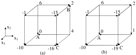
Fig. 1. Unit 3-dimensional cubes: oriented arcs indicate decreasing directions forJ(x)when (a) J(x)is CLG-function or (b)J(x)is CU-function. Solutionsx= (0,0,0)andx= (1,1,0)(pointAandBin (a)) are two local minima for the 2-facex1-x2withx3= 0. In both cases, the global minimum isx= (1,0,1)(pointC).
Example 1: Consider the set B3={0,1}3 and the team objective function J(x) : B3 7→ Z, taking on the values displayed in Fig. 1.a. The explicit expression of the function
J according to the formula (1) is
J(x) = 4x21+ 4x22−8x1x2+ 2x2
| {z }
J(x1,x2)
−10x3−10x1x3+3x2x3,
where we denote byJ(x1, x2)the function obtained
consid-ering the only terms in x1 and x2. In Fig. 1.a, the oriented
arcs indicate the decreasing directions for the team objective functionJ(x). FunctionJ(x)is a CLG-function as it has a unique local (global) minimum inB3 which isx= (1,0,1)
(pointCin the figure). However note thatJ(x1, x2)is not a
CLG-function as it has two local minima inB2. For instance, see the 2-facex1-x2withx3= 0which has two local minima
in x = (0,0,0) and x = (1,1,0) (point A and B). We complete the example by considering a different function
ˆ
J(x) :B37→Z, taking on the values displayed in Fig. 1.b. The explicit expression is
ˆ
J(x) =x21+ 4x22−5x1x2+ 2x2
| {z }
ˆ J(x1,x2)
−10x3−10x1x3+ 3x2x3,
where againJˆ(x1, x2)is obtained considering the only terms
in x1 and x2. In Fig. 1.b, the unique global minimum is
to such a situation we also have that Jˆ(x1, x2) is a
CLG-function onB2 as it has a unique local minimum inB2(see the 2-face x1-x2 withx3 = 0 which has a local minimum
inx= (0,0,0) (pointA)).
A special case of completely unimodality is whenf(.)is monotonic along any single direction, which corresponds to being both left hand side of (4) and (5) positive. Now, f(.)
is monotonic along any single direction, when for all i = 1. . . , n, one of the following mutually exclusive conditions holds true
max x∈Bn
∂J(x)
∂xi
<0 (6)
min x∈Bn
∂J(x)
∂xi
>0. (7)
We can specialize Corollary 1 to such a particular case. Lemma 2: (Sufficient conditions) If the team objective function J(x) is such that, for alli ∈N, one between (6) or (7) hold, then
1) the team optimum is
x∗i =
(
1 ifmaxx∈Bn∂J(x)
∂xi <0
0 ifminx∈Bn ∂J(x)
∂xi >0
2) the team optimumx∗is also the unique pbp optimum, 3) any pbp optimization algorithm converges to the team
optimum x∗ in at mostn iterations.
Proof: Item 3 is straightforward from item 2. To prove item 1 and 2 consider that ifmax∂J∂x(xi)<0, then ∂J∂x(xi) <0
for allx. Analogously, ifmin∂J∂x(x)
i >0then
∂J(x)
∂xi >0 for allx.
Let us finally observe that verifying whether (6) or (7) holds is easy (polynomial inn), as we just have to find the maxima, respectively the minima, of the nfunctions ∂J∂x(xi) linear inx∈Bn.
IV. GENERALIZATION TOmBmOPTIMIZATION Let us now generalize the results established in the preceding section to the case where DMs make decisions sequentially in groups ofm.
Theorem 1: (Sufficient conditions) Letx∗=1be an(m− 1)b(m−1) optimum, if the team objective functionJ(.)is such that for allS⊆N with|S|=mit holds
max
x∈BnRSJ(x)<0 (8) then
1) x∗ is the team-optimum
2) x∗ is also the uniquembm optimum,
3) any mbm optimization algorithm converges to the team-optimum x∗.
Proof: Item 3 is straightforward from item 2. To prove item 1 and 2, let us assume by contradiction that there exists a team optimum value x∗ 6=1. Let V ={i:x∗
i = 0}. The
cardinality ofV cannot be greater than or equal tom. Indeed considerS⊆V with|S|=m, sinceRSJ(x∗)<0 implies
J(x◦) < J(x∗), where x◦ ∈ Bn differs from x∗ only for
the components in S, i.e., x◦
i = 0 if i ∈ V \S, x◦i = 1
otherwise. Thenx∗ should be within an Hamming distance
strictly less than m from 1, but this situation cannot occur since1by definition is optimum within its neighborhood of radiusm−1.
Example 2: Consider the team objective functionJ(x) =
x1+x2−3x3−5x1x2+x1x3+x2x3.The solutionx∗=1
is a pbp optimum as, for alli,bi+Pk6=iaik<0. Since for
allS, with|S|= 2condition (8) holds (fori= 1andj= 2, we haveb1+b2+a12+ maxx∈Bn(a13+a23)x3=−1), then
x∗=1is also team-optimum.
Remark 3: In the above lemma, the assumption x∗ =1 is without loss of generality. Actually, if the team problem has a unique team optimum x∗ 6= 1 then the following transformation can be applied to the decision space such that the new team optimum isxˆ∗= 1:
ˆ
xi=
½
xi if x∗i = 1 1−xi itx∗i = 0.
(9)
Let us finally observe that verifying whether (8) holds is, for fixed m, polynomial in n although exponential in m, as we just have to find the maxima of the ¡mn¢ functions
RSJ(x)linear inx∈Bn.
V. SUB-MODULARTEAMPROBLEMS
In the past sections we have provided conditions for the convergence from any initial state x(0). Now, we show that we can recognize in polynomial time a special class of sub-modular team problems, which do not meet the aforementioned conditions and for which the convergence is guaranteed at least when the pbp algorithm is opportunely initialized. This class is characterized by so-calledthreshold strategies.
Let us callsub-modular team problems, all team problems with sub-modular team objective function. From [4], we remind from that i) a pseudo-Boolean functionf(.) is sub-modulariff(v) +f(w)≤f(vw) +f(v∨w)ii) a quadratic pseudo-Boolean functionf(.)is submodular iff its quadratic terms are nonpositive. However, from the following example, it is apparent that sub-modularity alone does not guarantee the convergence of any pbp optimization algorithm.
Example 3: Consider the sub-modular team objective function J(x) =x1+x2−3x1x2 and take x(0) = (0,0).
The team optimum is(1,1)but observe that at iteration 1, no DM alone benefits from changing its decision from 0 to 1. Hence the pbp optimization algorithm starts and terminates in(0,0).
We can generalize the above reasoning to show that sub-modularity alone does not guarantee the convergence of any
mbm optimization algorithm. On this purpose, note that if the team objective function is sub-modular, then condition (8) reduces to
X
i∈S
bi+
X
i,j∈S
aij <0, for allS, with|S|=m. (10)
We derive the above result by reminding that all quadratic terms are nonpositive and therefore maxxPk6=i,j(aik +
Example 4: Consider the sub-modular team objective functionJ(x) = 2x1+ 2x2+ 2x3−3x1x2−3x1x3−3x2x3
and take x(0) = (0,0). The team optimum is again (1,1)
but observe that at iteration 1, no pairsiandjof DMs alone benefits from changing their decisions from 0 to 1. Note that condition (10) form= 2becomesbi+bj+aij <0and there
is no pairi andj that satisfies such a condition. Hence the
mbmoptimization algorithm starts and terminates in(0,0). A. A Special Class with Threshold Strategies
Threshold strategy means that a DM i chooses xi = 1
if and only if at least other li DMs do the same. The
following simple example shows that when players (DMs) have threshold strategies the team objective function is sub-modular. The team objective function is as in (1). We say that player ihas a threshold strategy with thresholdli=k,
if its strict pbp strategy is
µi(x−i) = ½
1 if kx−ik1≥k
0 otherwise. (11)
Lemma 3: If all players have threshold strategies then the team objective functionJ(x)must be sub-modular.
Proof: Observe that playeri has a threshold strategy with li = k. Denote by S(k) the set of all subsets of N,
which do not contain DM i and have cardinality less than
k. Now, for a generic subset S ∈ S(k), take x−i such that
xj = 1for all j ∈S and xj = 0 for allj ∈N\(SS{i})
and observe that from (11) it must hold that µi(x−i) = 0.
But this means that the following condition holds true
bi+
X
j∈S
aij ≥0 for allS∈ S(k). (12)
Repeat the same reasoning considering a generic subsetS ⊆
N\ S(k), and take x−i such thatxj= 1 for allj∈S with
j6=iandxj= 0for allj∈N\S. Observe that from (11) it
must hold thatµi(x−i) = 1which implies that the following
condition hold true
bi+
X
j∈S
aij <0 for all S⊆N\ S(k). (13)
Now, consider two setsS1∈ S(k)with|S1|=k−1 and
S2=S1∪ {j} ∈N\ S(k). Observe thatS2has cardinality
|S2|=kas it is obtained fromS1by adding a single DMj.
We complete the proof by observing that for (12) and (13) to be valid it must be aij < 0 for all i and j. Then J(.)
has all quadratic terms negative which proves that J(.) is sub-modular.
This special class of sub-modular team problems is in-teresting as i) threshold structures can be recognized in polynomial time and ii) any pbp optimization algorithm initialized at x(0) =1 converges to the team-optimum x∗, in general different from 1, as established in the following theorem.
Theorem 2: There exists a polynomial algorithm that ver-ifies conditions (12) and (13) in O(n2logn). In case of positive answer, any pbp optimization algorithm initialized atx(0) =1converges to the team-optimum.
Proof: (Complexity) Given a DMi, consider all DMs except i in the order σ(1), . . . , σ(n) with aiσ(1) ≤ . . . ≤
aiσ(n). We remind here that the ordering process has a
complexity O(nlogn). Now, conditions (12) and (13) are verified if and only ifbi+aiσ(1)+. . .+aiσ(k−1)≥0 and
bi+aiσ(n−k)+. . .+aiσ(n)<0. We can limit ourselves to
verify the latter two conditions for any possible value of the thresholdlifrom 1 ton. Such a procedure is carried out via a
dicotomic search and has a complexity ofO(logn). Then, for fixedithe total complexity isO(nlogn) +O(logn), and as
O(nlogn)dominates (is always greater than) O(logn) the total complexity simply reduces to the cost of the ordering processO(nlogn). We conclude our proof by noticing that the ordering process must be repeated n times (one for all DMi) and therefore the resulting complexity isO(n2logn).
(Convergence of pbp) Assume DMs ordered by increasing thresholds, i.e.,l1≤. . .≤ln. Starting atx(0) =1any pbp
optimization algorithm converges to the pbp optimum nearest to1(in terms of Hamming distance), call itxˆ. In other words
ˆ
x= arg min{kx−1k: xis pbp-opt.}. We must show that
ˆ
xis also the team-optimum. To prove this fact corresponds to proving that, if there exists a second pbp optimum, call it
˜
x, it must hold
J(ˆx)−J(˜x) = RSJ(˜x) = = X
i∈S
bi+
X
i,j∈S
aij+
X
r6∈S
X
i∈S
air˜xr≤0,
whereS is the set of components which are zero inx˜ and one inxˆ. Now note thatPi,j∈Saij+Pr6∈S
P
i∈Sairx˜r=
P
i∈S
Pn
r=1airxˆr and therefore we can rewrite the above
inequality as
J(ˆx)−J(˜x) =X i∈S
(bi+ n
X
r=1
airxˆr) =
X
i∈S (bi+
X
r∈S¯
air)≤0,
(14) where we denote byS¯the set of components which are one inxˆ. Then we need to prove the validity of (14). Now, note that if DMs are ordered by increasing thresholds, it must holdx˜≤xˆcomponent-wise. Hence, asxˆ is a pbp optimum then eachi∈S has thresholdli<kxˆ−0k=kxˆk which in
turns implies thatPi∈S(bi+Pr∈S¯air)≤0 and therefore
(14) hold true.
VI. NUMERICAL EXAMPLE
In this first example we simulate a pbp optimization and show that the algorithm converges to the team optimum. Consider the following team objective function
J(x) = −x1+x2+x3+x4+ 5x5−2x1x2+ 4x1x3+ + 2x1x4−4x1x5−6x2x3−2x2x4−7x4x5
By direct verification, it can be proved that the above function is a CLG-function as it has a unique local minimum in (1,1,1,1,1). Similarly, we can see that it is not a CU-function as, for instance, on the 2-facex1-x3withx2=x4=
x5= 0, conditions (4)-(5) are both verified. The function is
TABLE I
SEQUENCE OFDMS’DECISIONS:BLOCKS ON THE LEFT,MIDDLE AND RIGHT DESCRIBE THE FIRST,SECOND AND THIRD ROUND OF OPTIMIZATION.
DM xi x J(x) DM xi x J(x) DM xi x J(x)
1 1∗ (1,0,0,0,0) -1 1 0∗ (0,1,1,0,0) -4 1 1∗ (1,1,1,1,1) -7
2 1∗ (1,1,0,0,0) -2 2 1 (0,1,1,0,0) -4 2 1 (1,1,1,1,1) -7
3 1∗ (1,1,1,0,0) -3 3 1 (0,1,1,0,0) -4 3 1 (1,1,1,1,1) -7
4 0 (1,1,1,0,0) -3 4 1∗ (0,1,1,1,0) -5 4 1 (1,1,1,1,1) -7
5 0 (1,1,1,0,0) -3 5 1∗ (0,1,1,1,1) -6 5 1 (1,1,1,1,1) -7
TABLE II
SEQUENCE OF DECISIONS:FIRST AND SECOND ROUND OF PBP OPTIMIZATION(LEFT AND MIDDLE BLOCKS), 2B2OPTIMIZATION(RIGHT BLOCK).
DM xi x J(x) DM xi x J(x) DM xi x J(x)
1 0 (0,0,0,0,0) 0 1 0 (0,0,1,0,0) -3 1-2 1∗
−1∗ (1,1,0,0,0) -3 2 0 (0,0,0,0,0) 0 2 0 (0,0,1,0,0) -3 3-4 1∗
−1∗ (1,1,1,1,0) -11 3 1∗ (0,0,1,0,0) -3 3 1 (0,0,1,0,0) -3 5-1 1∗
−1 (1,1,1,1,1) -23 4 0 (0,0,1,0,0) -3 4 0 (0,0,1,0,0) -3 2-3 1-1 (1,1,1,1,1) -23 5 0 (0,0,1,0,0) -3 5 0 (0,0,1,0,0) -3 4-5 1-1 (1,1,1,1,1) -23
Start from the decision vectorx= 0and assume that the DMs make their decision in the following order: DM 1, DM 2,. . ., DM 5. Table I reports the sequence of DMs’ decisions (decisions are starred when they change with respect to the previous round). Blocks on the left describe the first and second round of optimization while block on the right describes the third round of optimization.
If we consider only the vectors x that change from a decision to another one we obtain the sequence
σ = (1,0,0,0,0),(1,1,0,0,0),(1,1,1,0,0),(0,1,1,0,0),
(0,1,1,1,0),(0,1,1,1,1),(1,1,1,1,1).
In this second example we simulate the pbp and the 2b2 optimization for the following team objective function and show that only in the second case we converge to the team optimum:
J(x) =x1+x2−3x3+x4+x5−5x1x2+x1x3+x2x3+
−4x1x4−4x1x5−4x2x4−4x2x5−5x4x5.
First observe that the solution x∗ = 1 is a pbp optimum as, for all i, bi+Pk6=iaik <0. Furthermore, since for all
S, with |S| = 2 condition (8) holds, then x∗ = 1 is also
team-optimum. The pbp optimization is carried out as in the previous example and decisions are reported in Table II (left blocks describe the first and second round). Convergence is onx= (0,0,1,0,0)6=x∗. Differently, the 2b2 optimization
converges to x∗ as evident from the sequence of decisions
listed in the right block.
VII. CONCLUDINGREMARKS
In future works, we wish to extend the obtained results to consensus problems. Actually, consensus problems have been recently reinterpreted as special potential games [11]. For these games there exist algorithms, very similar in spirit to pbp algorithms and called best response path algorithm, that guarantee the distributed convergence to Nash equilibria. A second line of research aims at providing a parallel betweenmbmand self organizing/Kohonen maps, since both
are optimization methods that can be applied to boolean spaces with decreasing goal functions that in each iteration modify a subset of decision variables.
REFERENCES
[1] B. Bamieh, F. Paganini, and M. A. Dahleh, “Distributed control of spatially invariant systems”,IEEE Transactions on Automatic Control, vol. 47, no. 7, pp. 1091-1107, July 2002.
[2] B. Bamieh and P. G. Voulgaris. “A convex characterization of dis-tributed control problems in spatially invariant systems with commu-nication constraints”,Systems and Control Letters, vol. 54, no. 6, pp. 575-583, June 2005.
[3] D. Bertsimas, A. Thiele, “A Robust Optimization Approach to Inven-tory Theory”,Operations Research, vol. 54, no. 1, January-February 2006, pp. 150-168.
[4] E. Boros and P. L. Hammer, “Pseudo-Boolean optimization”,Discrete Applied Mathematics, vol. 123, pp. 155-225, 2002.
[5] H. Bj¨orklund and S. Sandberg and S. Vorobyov, “Optimization on completely unimodal hypercubes”, Technical Report 2002-018, De-partment of Information Technology, Uppsala University, May 2002. [6] M. S. Branicky, V. S. Borkar and S. K. Mitter, “A Unified Framework for Hybrid Control: Model and Optimal Control Theory”,IEEE Trans. on Automatic Control, vol. 43, no. 1, pp. 3145, 1998.
[7] P. R. De Waal and J. H. Van Schuppen, “A class of team problems with discrete action spaces: optimality conditions based on multimodular-ity”,SIAM Journal on Control and Optimization, vol. 38, pp. 875–892, 2000.
[8] G.C. Goodwin and D.E. Quevedo, “Finite alphabet control and esti-mation”,International Journal of Control, Automation, and Systems, vol.1, no.4, pp. 412–430, 2003.
[9] P. L. Hammer and B. Simeone and T. Liebling and D. de Werra, “From linear separability to unimodality: a hierarchy of pseudo-boolean functions,SIAM Journal of Discrete Mathematics, vol. 1, pp. 174–184, 1988.
[10] Y.-C. Ho, “Team decision theory and information structures”, Pro-ceedings IEEE, vol. 68, pp. 644–654, 1980.
[11] J.R. Marden, G. Arslan, and J.S. Shamma, “Connections between cooperative control and potential games illustrated on the consensus problem”,European Control Conference, Kos, Greece, July 2-5, 2007, pp. 4604-4611.
[12] J. Matousek, “The number of unique-sink orientations of hypercube”, Combinatorica, vol. 26, no. 1, pp. 91–99, Feb. 2006.
[13] A. Rantzer, “Linear quadratic team theory revisited”,Proceedings of the 2006 American Control ConferenceMinneapolis, Minnesota, USA, June 14-16, pp. 1637–1641, 2006.