Valuation of derivative securities using stochastic analytic and numerical methods

(1)

Valuation of Derivative Securities using

Stochastic Analytic and Numerical

Methods

David Heath

A thesis submitted for the degree

of

Doctor of Philosophy

(2)

Declaration

I declare that, except where otherwise stated in the text the work presented in this thesis is my own.

.

(3)

I . .

Acknowledgement

(4)

Abstract

This thesis details methods and procedures to compute prices and hedging strategies for derivative securities in financial mathematics using stochastic analytic, numerical and variance reduction techniques.

Results are obtained on explicit hedge ratio representations for non-smooth payoff functionals and multidimensional diffusion processes with stopping boundaries. These methods are used to determine hedge ratios for the maximum of several assets and look-back options. A number of powerful variance reduction techniques are described. These include the use of measure transformations, discrete versions of importance sampling estimators, control variates based on Ito integral representations, stratified sampling and quasi Monte Carlo. For many of these techniques explicit formulas for the variance of the resulting estimators are obtained.

(5)

x

CONTENTS

Chapter 4: Valuation of European Bond Options

for Two-Factor Interest Rate Models ... 93

4.1 Two-Factor Stochastic Volatility Models ... 94

4.2 Pricing of Contingent Claims ... 97

4.3 Stochastic Numerical and Variance Reduction Methods ... 101

4.4 Application to the Extended Fong and Vasicek Model ... 105

4.5 Experimental Results for European Pricing ... 109

Chapter 5: Valuation of American Bond Options for Two-Factor Interest Rate Models ... 115

5.1 American Options for Two-Factor Bond Models ... 116

5.2 Representation of the Early Exercise Premium ... 118

5.3 Explicit Representation of the Early Exercise Premium for the Extended Vasicek Model ... 123

5.4 Computation of Terms for the Extended Vasicek Model ... 128

5.5 American Pricing for the Extended Fong and Vasicek Model ... 131

5.6 Computational Results for American Pricing ... 132

(7)

Preface

Most financial assets evolve in an uncertain manner over time and, as a result, the gen-eral theory of stochastic processes is viewed by many as providing the natural mathe-matical framework for the analysis, valuation and management of these securities. This theory, both in its discrete and continuous time forms, provides a powerful and unifying set of analytic tools which forms the basis of a growing number of successful applica-tions to financial markets. These applicaapplica-tions have their origins in the seminal work of Black & Scholes (1973), Merton (1973), and the arbitrage-free pricing methodology developed by Harrison & Kreps (1979), Harrison & Pliska (1981) and Duffie (1988).

The theory of stochastic processes when applied to derivative security valuations requires, in essence, three main problem areas to be addressed. Firstly, there is the challenge of finding suitable stochastic models that can represent the underlying secu-rities. Secondly, there is the problem of parameter estimation and fitting the model to actual market data. This task is usually integrated with procedures for using the model and is sometimes referred to as model calibration. Finally, there is the problem of computing prices and hedging strategies based on the models.

This thesis will focus on the third problem area - the development of pricing and hedging procedures for derivative securities with particular emphasis on the use of stochastic analytic, numerical and variance reduction techniques. The main aim is to show that these advanced mathematical tools can now be applied to solve a range of difficult and challenging valuation problems. For all of the applications described in this thesis, corresponding software systems have been built which deliver fast, reliable and accurate pricing and hedging of the corresponding security. The technology represents a significant improvement over existing methods and approaches.

A number of new results are included in this thesis. Some of these refer to new pricing methods, formulas and perspectives, and others refer to extension of existing methods but applied to new classes of problems. Also, each of the applications covered includes new development of the underlying theory. The overall theoretical framework proposed, which has been driven by real world applications, should be both of inde-pendent mathematical interest and of practical value as it can be successfully applied to a wide class of valuation and hedging problems.

(8)

XII

PREFACE

expressions for the integrands in Ito integral representations of contingent claim payoff structures. This result is established firstly for one-dimensional diffusion processes and is then extended for multidimensional diffusion processes with stopping boundaries. Using general results from the theory of measure and integration, conditions are found under which these results can be strengthened to include a wide class of non-smooth payoff functionals. These methods are applied by finding corresponding representations for one-dimensional absolutely continuous functionals, the maximum of several assets and lookback options.

A number of variance reduction techniques based on stochastic analytic techniques are outlined in Chapter 2. These methods are mainly used to improve the performance of the raw Monte Carlo estimator by finding new ones having the same expectation but smaller variance. Some new variance reduction methods will be described as well as extensions to, and new perspectives on, some existing or classical ones. These include the use of general measure transformation procedures, discrete versions of importance sampling estimators, control variates based on Ito integral representations and new ap-proaches to stratified sampling and quasi Monte Carlo. For a number of these methods, the variance of the resulting estimators is computed explicitly. This is of considerable practical value as it provides the basis for precise controls of the factors which contribute to the variance of an estimator.

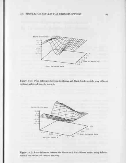
Pricing and hedging procedures for a class of foreign exchange barrier options under stochastic volatility are considered in Chapter 3. A general valuation methodology is developed using mean self-financing arguments and the minimal equivalent martingale measure. This methodology is then applied by computing the prices and hedge ratios of down-and-out calls for the Heston (1993) model. Fast and accurate valuations are obtained by using a combination of control and antithetic variates and stratified sam-pling techniques, together with a derivative free weak approximation. It is shown that these methods can be adapted to suit the observation frequency or fixings of the barrier option.

The pricing of discount bonds and European style contingent claims for multifactor term structure models is dealt with in Chapter 4. The approach is demonstrated by efficiently computing the prices of discount bonds and European call options on bonds for a version of the Fong & Vasicek (1991a,b) model. This version is extended to in-clude time dependent parameters in the drift term of the short rate for the model. It is shown that option prices and corresponding hedge ratios can be computed using repre-sentations under the so-called forward measure together with appropriate combinations of stochastic and deterministic numerical methods.

(9)

III

PREFACE _XIII

together with appropriate stochastic and deterministic numerical methods, to compute the prices of American puts for the two-factor extended Fong & Vasicek (1991a,b) model considered in Chapter 4. A number of simulation experiments are described which show that both American option prices and the corresponding two-dimensional critical exercise boundary can be efficiently estimated.

Some of the main characteristics which distinguish the use of numerical methods in this thesis compared to some previous treatments of the subject include the following: Firstly, and most importantly, these techniques are based mainly on the application of stochastic analytic principles and the semimartingale calculus. This approach has enabled new theoretical insights to be gained and provides support and a rigorous mathematical framework for a wide class of valuation and hedging problems to be handled. In fact the successful application of these methods has only been achieved by using some of the most powerful and deepest results from stochastic analysis, supported by a range of other techniques from numerical analysis and general simulation. It has also meant that the detailed structure of specific models can be more easily exploited. Secondly, the systematic application of higher order numerical approximations is emphasized. For example, excellent results have been achieved with derivative free, predictor-corrector and extrapolated schemes, described in Kloeden & Platen (1992) and Hofmann, Platen & Schweizer (1992).

Thirdly, variance reduction, based on the combined use. of several procedures has been used. Previous researchers have applied usually one or two separate techniques,. typically antithetic and control variates from general simulation. However huge overall gains can be achieved by building systems which combine a number of complementary methods. For example, as will be explained in Chapter 2, finite-difference approxima-tions can form the basis of control variate estimates in stochastic simulaapproxima-tions and these can be combined with quasi Monte Carlo techniques.

Finally the theory developed in this thesis has been specifically designed to cater for multidimensional pricing problems and models. This type of modelling is increasingly required for many types of path-dependent and global securities, groups of assets, and even single instruments, where either the drift or diffusion components are themselves stochastic. All of the applications covered in Chapter 3 to 5 are based on multidimen-sional models.

The numbering system used in this thesis is as follows: Equations are numbered by their section and number in the section in parentheses where the reference occurs within the same section or chapter. The chapter number appears as a prefix, with the full reference (again in parentheses) when the equation is referred to in other chapters. All figures, lemmas and theorems are numbered by their chapter, section and order of appearance within a section and do not appear in parentheses. Except for Section 1.4 the use of lemmas, propositions and theorems is avoided. This is to provide a more descriptive and expository account and a style of presentation which encourages a more appropriate discussion of the practical features of the methods used and their results.

1 I

I

I I

(10)

A Brief Survey of Numerical Methods in Finance

Background

There is now considerable interest both from academics and practitioners in the appli-cation of stochastic modelling and other advanced mathematical methods to support the pricing and management of derivative securities in the finance area. A derivative se-curity or contingent claim is one the value of which is dependent on, or is derived from, some other underlying asset or security such as a bond, stock or currency contract. Over the last decade the growth in the use of derivative securities has been enormous. Financial institutions are seeking new products, new ways of handling existing ones and better methods for managing the risks associated with trading in these instruments.

In the past, because of the intractability of the underlying stochastic models, the development of accurate pricing methods has been extremely difficult. Analytic solu-tions to valuation problems are possible only in a few specialized cases, for example the classical Black and Scholes model based on a single asset and geometric Brownian motion. Consequently, numerical techniques are required for many types of valuation problems.

The use of discrete time methods including the application of stochastic numerical procedures, is in some sense fundamental and natural to an understanding and treat-ment of financial markets because individual financial securites are in fact observed and traded at discrete points in time. The continuous time theory is however extremely useful in providing a more concise formalism, clarifying insights and asymptotic limits to valuation problems.

The rapid development of new derivative securities and corresponding methods for pricing and managing them can be expected to continue in the future with particular emphasis on multidimensional modelling, complex payoff structures and the integration of risk management procedures over many instruments and even across divisions within financial institutions. For these type of challenges it is likely that both stochastic and deterministic numerical methods will play an increasingly important and crucial role.

Numerical approximations are now widely used in the finance industry. Even in cases where so-called exact valuations exist, computations based on these valuations are often supported by an array of deterministic numerical procedures such as interpolation, equation solving, search techniques, differentiation and integration routines. These numerical methods have become more effective in recent years due to increases in the power of desktop workstations and computers, at reduced costs, and the widespread availability of comprehensive numerical software packages, both in the commercial and

(11)

XVI BRIEF SURVEY OF NUMERICAL METHODS IN FINANCE public domains.

Broadly speaking three main categories of numerical approximations have been used for the valuation of derivative securities. These are finite-difference methods, multinomial lattices and Monte Carlo simulation. In addition, a number of analytic approximations have been proposed and applied to valuation problems.

Finite-Difference Approximations

Finite difference approximations are used to solve numerically the Kolmogorov back-ward or Feynman-Kac equation with associated boundary conditions. Subject to cer-tain integrability and smoothness conditions, this partial differential equation must be satisfied by the valuation process viewed as a function of time and the state variables in the underlying model. In the case of American options, a free boundary problem arises which can also be expressed as a variational inequality.

The method in its implicit form was first applied to option valuation problems by Schwartz (1977) and Brennan & Schwartz (1977). The valuation of derivative securities using explicit finite-difference methods has been analysed by Hull & White (1990) and described in the monograph by Hull (1993). The relationship between option pricing and the Feynman-Kac formula has been explored by Duffie (1988) and in a wider context by Karatzas & Shreve (1988). The monograph by Wilmott, Dewynne & Howison (1993) provides a comprehensive and accessible introduction to the use of partial differentiation equation solution techniques in finance. Dempster (1994) and Dempster & Hutton (1994) present some recent and encouraging results on the use of finite-difference and related approximations for the valuation of a range of option securities. These results focus on the use of linear programming techniques combined with matrix factorization.

Also of interest is the method of lines applied to general multidimensional free boundary problems by Meyer (1977) and used for American pricing by Carr & Faguett (1994) and Meyer & van der Hoek (1994). This technique, related to finite-difference methods, usually involves discrete time approximations of the underlying partial dif-ferential equations by ordinary differential equations. In the case of multidimensional pricing, some discretization of one of the state space variables is needed and this results in a set of equations which must be solved or numerically evaluated at each time step. For the Black and Scholes model these resulting ordinary differential equations can be solved explicitly and the approach is then referred to as the analytic method of lines.

Finite-element methods can also be used to approximate the solutions of a wide class of partial differential equations. Because of the relative ease with which boundary conditions can be handled, they are better suited to free boundary problems and there-fore to the pricing of certain types of American options. A description of these methods can be found in most books on numerical analysis, for example Burden & Faires (1993) and Hoffmann (1992). In addition Wilmott, Dewynne & Howison (1993) provide

(12)

-BRIEF SURVEY OF NUMERICAL METHODS IN FINANCE XVII

formation on the formulation of the finite-element method for American pricing.

Lattice Methods

Binomial and multinomial lattice techniques constitute a popular and widely used numerical procedure for pricing a range of derivative securities. The basic binomial method values a derivative security by approximating the underlying diffusion with binomial trees for each process component where at each time step model components can move to at most two new values. The method was introduced for option pricing

by Cox, Ross & Rubinstein (1979). Usually the technique is applied backwards in time and when used to price American options represents an application of the Bellman principle of dynamic programming. A faster version of the method has been developed

by Breen (1991).

Approximation of the underlying diffusion by multinomial trees, where model com-ponents can move to a finite number of new states or values, leads to corresponding multinomial lattices. Trinomial and multinomial lattices have been analysed by Boyle (1988), Omberg (1988) and Boyle, Evnine & Gibbs (1989).

The application of binomial lattice methods to option valuations with transaction

costs has been examined by Boyle & Vorst (1992) and more recently by Mercurio & Vorst (1995a,b), who apply Schweizer's (1988, 1991, 1993) principle of risk-minimization for incomplete markets. Boyle & Lau (1994), and Cheuk & Vorst (1994b) apply bi-nomialla:ttices to the valuation and hedging of barrier options. Hull & White (1993) use an implicit two state variable binomial model to price lookback options. Their

approach is simplified by Cheuk & Vorst (1994a).

Monte Carlo Simulations

The application of Monte Carlo methods to option pricing was first described by Boyle (1977). According to the arbitrage-free pricing theory the price of many types of contingent claims can be expressed as the discounted expected value of its terminal future payoff under an appropriately changed probability measure. A standard Monte Carlo procedure would estimate this price by simulating many trajectories for the underlying stochastic model using this measure. The Monte Carlo estimate is then the discounted sample mean of the terminal payoffs for these simulated trajectories.

Monte Carlo simulations are used by both academics and practitioners to provide

comparative results for other methods and 'rough' estimates when no other valuation procedure is available. Since the pioneering work of Boyle, several authors have applied the technique to a variety of valuation problems. These include Hull & White (1987, 1988), Johnson & Shanno (1987) and Scott (1987) on stochastic volatility, Schwartz & Torous (1989) on mortgage-backed securities and Kemna & Vorst (1990) on the valuation of Asian options. Hofmann, Platen & Schweizer (1992), Duffie (1992) and

i

(13)

XVIII BRlEF SURVEY OF NUMERICAL METHODS IN FINANCE

Duffie & Glynn (1992) have also applied Monte Carlo methods for derivative security valuation problems.

For a number of valuation problems the pricing functional can be expressed as an integral involving the densities of the underlying model components. If these densities have an explicit form, the general methods of quasi Monte Carlo can be applied. These methods are described in the monographs by Ripley (1983) and more recently Nieder-reiter (1992). Their applicability to financial modelling problems have been examined by Joy, Boyle & Tan (1995). Quasi Monte Carlo in its standard form involves replacing pseudo-random numbers with so-called low discrepancy point sets such as Sobol (1967)

or Halton (1960) sequences. These low discrepancy sequences exhibit less deviations from uniformity compared to pseudo random numbers. Quasi Monte Carlo, in cases

where densities of the model components can be determined, seem to be well-suited

to higher dimensional problems. A version of quasi Monte Carlo involving the use of multipoint" random variables is considered in Chapter 2 of this thesis.

Recently Hofmann, Platen & Schweizer (1992), using measure transformation

tech-niques, and Clewlow & Carverhill (1992, 1994), using discrete versions of a martingale

control variate, have introduced powerful variance reduction methods which

signifi-cantly improve the performance of the raw Monte Carlo estimator. The paper by Hofmann, Platen and Schweizer is particularly significant as it represents the first

. successful attempt to formulate and use variance reduction techniques for financial modelling problems based on stochastic analytic methods.

The application of Monte Carlo methods in general simulation has been described by several authors. Some excellent references include Hammersley & Handscomb (1964) Ripley (1983), Bratley, Fox & Schrage (1987), Ross (1991) and Law & Kelton (1991). All of these sources provide information on variance reduction techniques. It is

some-what surprising that, since the work of Boyle (1977), these classical methods have only recently been used systematically in the finance area.

Analytic Approximations and Related Methods

Analytic approximations have been used for both European and American option val-uations. Some examples of these in the case of American options include the quadratic

approximation method developed by MacMillan (1986) and Barone-Adesi & Whaley

(1987), the compound option approach used by Geske & Johnson (1984) and refined

by Bunch & Johnson (1992). McKean (1965), Kim (1990), Jacka (1991), Carr, Jarrow

& Myneni (1992) and Chesney, Elliott & Gibson (1991) price American options as the

sum of the corresponding European price together with an integral representation of

the early exercise premium. This representation is exact but requires a backward

nu-merical technique to determine the optimal exercise boundary and from this the price of the option. Examples of analytic approximations using Taylor series expansions and

(14)

•

BRIEF SURVEY OF NUMERICAL METHODS IN FINANCE _XIX

White (1988).

Laplace transform methods have been used to value Asian options by Geman & Yor (1992) and Eydeland & Geman (1995) and Parisian options by Chesney, Jeanblanc-Picque & Yor (1995). Inversion of the Laplace transform for Parision options requires some delicate numerical problems to be solved. These problems together with methods for handling them are presented by Cornwall et al. (1995). The fast Fourier transform is used by Carverhill & Clewlow (1990) to evaluate Asian options.

Performance Criteria

The performance of a numerical method is measured in terms of its speed, accuracy, flexibility, robustness and ease of implementation. The attribute of speed is related to the rate of convergence of the numerical method to a continuous time limit and is clearly of considerable importance to financial institutions. This is because these institutions often have large books of securities which must be frequently revalued and

hedged. Also, sensitivity analysis studies, model calibration procedures and calculation of implied parameters often require numerically intensive computations.

The requirements for fast valuations must be balanced with the competing

de-mands of aceuracy which, for financial modelling problems; usually varies considerably, depending on the application. For example, if hedge ratios are being computed using finite difference approximations, the underlying valuation procedures may need to be very accurate. On the other hand, sensitivity analysis work may require less accuracy with more emphasis being placed on providing rapid feedback to risk managers. Also

the requirements for accuracy need to be worked out for the entire valuation problem not just for a particular component. Clearly if the parameter estimation and mod-elling errors associated with a product are say, of the order of 5 per cent, which may easily arise for new products and certain types of exotics, it is of limited value having valuation software that is accurate to say 0.1 per cent.

The flexibility of a numerical method refers to how easily the method can be adapted to new problems and situations. This attribute is particularly important to institutions

at the cutting-edge of research and development.

Robustness is measured in terms of the stability of the corresponding method. A numerical method is stable if small changes in input parameters lead to small changes in output results. Some algorithms are stable in certain regions and not in others. The differences in the modes of convergence and dynamics of stochastic processes lead

to different stability criteria for stochastic systems, see for example Kloeden & Platen (1992). An important part of the work required to build valuation procedures based on stochastic numerical methods is therefore a detailed and systematic study of stability issues relating to the dynamics of the underlying stochastic system.

Finally, we can measure the ease with which a numerical method can be formulated and implemented within a subroutine library or separate application. This is related to

I

(15)

xx

BRIEF SURVEY OF NUMERICAL METHODS IN FINANCE

the complexity of the method and its capacity to be modularized and broken down into components. This is also an important attribute as software development expenditure can be considerable with time and cost overruns common.

If the various classes of numerical methods are compared and evaluated in terms of their performance, it is found that in general the fully numerical techniques are more flexible but slower and less accurate compared to analytic approximations. Stability problems depend on the specific application being considered but are more likely to be an issue for fully numerical techniques compared to analytic approximations. There are considerable differences between the methods in terms of their ease of implemen-tation. For example quadratic approximations for American options can usually be implemented in a straightforward manner, whereas the integral representation of the early exercise premium seems to require more delicate numerical problems to be solved. As observed by Brennan & Schwartz (1978), multinomial lattice approaches can be regarded as versions of explicit finite-difference methods. The methods are therefore roughly similiar in terms of their performance capabilities. However Geske & Shastri (1985) compare the two approaches and note some differences in efficiences for different types of applications. The main disadvantage of finite-difference and lattice approaches is that memory requirements explode exponentially with increases in the dimensionality of the model and the number of branch points used. The speed of convergence to a continuous time limit can also be extremely slow, particularly for certain classes of path dependent options. Cheuk & Vorst (1994a,b) report very slow convergence of binomial pricing methods for barrier and lookback options. Their research in the case of look back options also indicates the sensitivity of valuations to the observation frequency of the option.

Monte Carlo techniques are generally considered to be flexible and in their basic form simple to implement although somewhat inefficient. Compared to lattice and finite-difference methods they seem to be better suited to higher dimensional problems. A common view, see for example Hull (1993) and Reider (1994) is that they are not as effective for American pricing. However Clewlow & Carverhill (1992, 1994) and Grant, Vora & Weeks (1993) have applied Monte Carlo techniques to American valuations. As will be demonstrated in this thesis, a two-factor American problem is handled using techniques related to Monte Carlo simulation. An excellent comparison and evaluation of various approximation methods for American options together with a description of a new approximation technique based on capped options is given by Broadie & Detemple (1994).

(16)

.

-Chapter 1

Calculation of Hedge Ratios

for Non-Smooth Payoff Functionals

The calculation of hedge ratios is fundamental to both the arbitrage free valuation of derivative securities and also the risk management procedures needed to replicate these instruments. In this chapter we consider the problem of finding explicit Ito integral representations of the payoff structure of a derivative security. If such a representation can be found in an explicit form, the corresponding hedge ratio can usually be easily

identified and calculated.

In Section 1.1, following from the work of Bensoussan (1984), Karatzas & Shreve (1988), and Hofmann, Platen & Schweizer (1992), we propose a general framework which expresses the price dynamics of a derivative security as the conditional expecta-tion, under a suitable measure, of the payoff structure of the security. This framework will be used through?ut this thesis.

In Section 1.2 and 1.3 we apply the Markov property and the Kolmogorov back-ward equation to obtain explicit Ito integral representations for a class of smooth payoff functionals, firstly for one-dimensional diffusion processes and, secondly, for multidi-mensional diffusion processes with stopping boundaries. The extension to include stop-ping boundaries is needed to support the pricing and hedging of American options. These representations are related to the formula of Clark (1970) and results obtained by Haussmann (1979), Ocone (1984), Elliott & Kohlmann (1988) and Colwell, Elliott & Kopp (1991).

Applying general arguments from the theory of measure and integration, we then extend these results in Section 1.4 to include a wide class of non-smooth payoff func -tionals which can be expressed as the pointwise limit of smooth func-tionals that satisfy a uniform linear growth bound. In Section 1.5 we use these results together with certain smoothing operators to obtain explicit Ito integral representations for one-dimensional absolutely continuous functionals whose derivative is continuous except at a finite num-ber of points. In the last two sections of this chapter we extend these results to include representations of the maximum of several assets and lookback options. The represen-tation of the maximum of several assets provides an important tool for the compurepresen-tation of hedge ratios in the funds management area. In the case of lookback options we pro-vide an example of how these methods can be adapted to the case of path-dependent options.

(17)

2 CHAPTER 1. CALCULATION OF HEDGE RATIOS

1.1 Contingent Claim Pricing Fundamentals

Let W

=

(WI, . .. , wm) be an m-dimensional Brownian motion defined on the

proba-bility space (0, F, P). We assume that the filtration F = (Fk~to is the P-augmentation of the natural filtration of W. These conditions ensure, see Karatzas & Shreve (1988),

Proposition 2.7.7, that F satisfies the usual conditions.

Let Xto,:E.

=

{XiO,:E.

=

(X;,to,:E., ... , x:,to,:E.) , to ::; t ::; T} be a d-dimensional diffusion

process whose components satisfy the stochastic differential equation

m

dX;,to,:E.

=

ai(t, Xto,:E.) dt

+

L

bi,j (t, Xto,:E.) dW! (1.1) j=1

for to ::; t ::; T, i E {I, ... , d}, where Xto,:E. starts at time to with initial value J!.

=

(J!.I' ... ,bt) E ~d, and ~d is the set of d-dimensional reals. We assume that appropriate

growth and Lipschitz conditions apply for the drift ai and diffusion bi,j coefficients so

that (1.1) admits a unique solution and is Markov, see for example Kloeden & Platen

(1992).

In order to model the time value of money and stochastic interest rates we take

the first component Xl,to,~

=

r

=

{rt, to ::; t ::; T} to represent some instantaneous

interest rate process and the second component X2,to,~

=

f3

=

{f3t, to ::; t ::; T}

to model the price movements of a riskless savings account. We assu~e this savings account f3 evolves according to the stochastic differential equation

df3t

=

rt f3t dt (1.2)

for to ::; t ::; T, where f3 starts at time to with initial value f3to

=

1. Note that (1.2) can

be solved explicitly yielding

(1.3)

for to::; t ::; T. The vector process xto,~ could include several risky assets and other

securities as well as components to provide for additional specifications or features of

the model such as stochastic volatility or averages of risky assets for Asian options. In order to build a framework that will support in particular American, and certain classes of exotic option valuations and hedging, we consider a stopping time formulation

as follows:

Let ro c [to, T] X ~d be some region with ro n (to, T] x ~d an open set and define

a stopping time T : 0 --7 ~ by

T

=

inf{t > to: (t, X:o,~) rf. ro}. (1.4)

Using the stopping time T we define the region

(18)

~

-1.1. CONTINGENT CLAIM PRICING FUNDAMENTALS ₃

r I

contains all points of the boundary of

rOW

hich can be reached by the diffusion

Xto,!!<. We now consider contingent claims with payoff structures of the form

where h :

r

1 -+ !R is some payoff function.

Using terminology that is applied mainly for American option pricing, we call the set ro the continuation region and r 1 the exercise boundary, which forms part of the stopping region. For a diffusion process Xto,!. with continuous sample paths, an option is considered 'alive' at time 8, to ~ 8 ~ T, if (8, X;o,!.) E roo On the other hand it is 'exercised' or 'stopped' at the first time 8, to ~ 8 ~ T, that (8,X;o,!.) touches r l . It is assumed that (to,;f) E

r

0 since otherwise the derivative security would be immediately 'exercised' .

For example if we take ro

=

[to, T) X !Rd which implies T

=

T and payoff structures of the form h(T, X~'!.) this formulation reduces to the case of a multidimensional European style contingent claim.

Applying the Markov property, the option pricing or valuation function u : ro u

r

l -+ !R corresponding to the payoff structure h(T, X;o,!.) is given by

(1.5)

for (t, x) E ro u r l, where

E

denotes expectation under an appropriately defined proba-· bility measure

P

. We will not discuss here how this measure

P

,

which is usually the risk neutral measure, should be determined. A good choice, the so called minimal equiva-lent martingale measure, which can be used both for complete and incomplete markets is described in Hofmann, Platen & Schweizer (1992); see also Foellmer & Schweizer (1991) and Schweizer (1991).

Define the discounted functions

h

:

r 1 -+ !R and

u

:

r 0 UrI -+ !R by

h(8,y) -1 h(8, y)

Y2

(1.6)

for (8, y) E

r

l, (t, x) E fo U fl with Y

=

(YI,'." Yd) E !Rd, where we recall that x2_,_to_,_!. represents the price movements of the riskless savings account {J.

Let zto,to

=

{Zio,to, to ~ t ~ T} be the solution of the stochastic differential equation

(1. 7)

for to ~ t ~ T, starting at time to with initial value to. We can write the solution to (1.7) in the form

(19)

4 CHAPTER 1. CALCULATION OF HEDGE RATIOS

for to::; t ::; T. This expression together with the uniqueness of the solutions of (1.1) and (1.7) shows that

(1.9)

and

(1.10)

for to ::; t ::; T. Using these equalities, (1.5), the Markov property, equation (1.3) and the assignment (3T

=

x;,to,~ with ;f2

=

I, we have

Ut

=

u(tI\T,xi~:;)

E

(exp ( -

l:T

r s

dS)

h

(z;/\T

,z:~

~o

,

x;/\T,x:t~)

)

E

(exp ( -

l:T

r s

dS)

h (

Z;/\T

,z:

~~o

,

x;/\T'x:~~~) I

Ft)

{3t/\T

E

(;T

h

(T,

X;o,~)

)

{3t/\T

E (h

(T

,

X;o,~))

for (t 1\ T, X:~:;) E

roo

Define the martingale M

= {M

t : to::; t ::; T} by

Mt =

E

(h(T

,

X;O'~) 1Ft),

(1.11)

(1.12)

for to::; t ::; T. We assume that an appropriate growth condition applies for

h

so that the conditional expectation in (1.12) is well-defined. Applying once again equation (1.9), the Markov property and the definitions of hand u we have

M

t

=

E (h

(T'

x;

/\T'x:~~~

)

1Ft)

(20)

1.2. HEDGE RATIOS FOR ONE-DIMENSIONAL DIFFUSIONS

for to ~ t ~ T.

=

U

(t /\

T

_,xtO_t_/\'_T~)

Consequently the ,B-discounted valuation process

U

=

{Ut = U (t /\ T,

X:~~)

,

to

~

t

~

T}

5

(1.13)

is a martingale. Also, from (1.11) we can determine values for the random variable Ut if corresponding values for ,BtM and Ut are known. Usually it is much more convenient to compute prices via the function U rather than u. This is mainly because the martingale property associated with U enables us to apply a number of powerful results from stochastic analysis. In particular, subject to certain integrability conditions, the price process corresponding to

u will admit an Ito integral representation

, and from this hedging parameters can be determined either in an implicit or explicit form.

We will not discuss here how these hedging strategies for general valuations can be formulated. Instead we refer the reader to the papers by Hofmann, Platen & Schweizer (1992) and Karatzas (1989) for a more complete coverage; see also Bensoussan (1984) and Karatzas & Shreve (1988). Some specific examples of hedging strategies are how-ever considered in Part II of this thesis dealing with applications.

The above-analysis leading in particular to equations (1.11) and (1.13) demonstrates that the valuation of contingent claims as given by (1.5) can be reduced to the case of valuations of the form '

(1.14)

for some payoff function

Ii :

r

1 -+!R. Consequently in the remaining part of this

chapter and the next we will assume this type of structure for our pricing and hedging problems.

In the special case where T

=

T and the payoff structure takes the form h(X:;'~) we will refer to the corresponding equations for (1.5) and (1.11)-(1.14) as the time-independent formulations.

1.2 Explicit Hedge Ratios for

One-Dimensional Diffusions

In this section, to allow for an easier and simpler exposition of the underlying ideas, we suppose W

=

{Wt, t ~ to} is a one-dimensional Brownian motion defined on the prob-ability space (fl, F, P). Consider the one-dimensional stochastic differential equation

dXt

=

a(t, Xd dt

+

b(t, Xt ) dWt (2.1)

for to ~ t ~ T. Here a, b: [to, T] x !R -+ !R are measurable functions which have linear growth, are Lipschitz continuous in x and whose partial derivatives have linear growth

j

I

,

I

(21)

6 CHAPTER 1. CALCULATION OF HEDGE RATIOS

and are Lipschitz continuous in x. We denote by Xto,;£

=

{X;O,;£, to ~ s ~ T} the solution of (2.1) starting at J< E R at time to, to ~ t ~ T.

In this section we consider a European style contingent claim with a payoff structure

of the form

for J< E R and terminal time T.

Subject to certain growth bounds applying for the function h these conditions for

the coefficients a and b ensure, see Kloeden & Platen (1992), that E((h(X~

'

;£))2)

<

00

and the process M

=

{Mt, to ~ t ~ T} defined by

(2.2)

for to ~ t ~ T, is a square integrable martingale and therefore admits a (Kunita &

Watanabe (1967)) representation of the form

Mt

=

Mo

+

rt

~s

dWs, ito

where ~ is an F-predictable process with

The process ~ is unique in the sense that if Mt

F-predictable process ~, then

(2.3)

Mo

+ Jt~ ~s

dWs for some other

A more general statement of this uniqueness property can be found in Karatzas &

Shreve (1988), Exercise 3.4.22.

Finding explicit expressions for the integrand ~ is of considerable practical value as it is closely related to the computation of hedge ratios in the theory of option pricing. Here we seek explicit characterizations based on an application of the Kolmogorov

backward equation.

Define the scalar function u: [to, T] x R -+ R by

u(t, x)

=

E(h(X~X)), (2.4)

for (t,x) E [to,T] x R. We assume that the function u is of class C1,3, that is, con-tinuously differentiable with respect to t and three times continuously differentiable in

x. Expanding u(T, X~,;£) = h(X~';£) by the Ito rule and applying the Kolmogorov

(22)

-...

1.2. HEDGE RATIOS FOR ONE-DIMENSIONAL DIFFUSIONS ₇

for to :S t :S T. Using the time-independent formulations of (1.12), (1.13) with T

=

T,

h

= Ii

and u

=

ii, and (2.5) we have

(2.6)

for to :S t :S T. This result can also be obtained by applying Ito's formula to

u(T, X~'~)

=

h(X~'~), taking the conditional expectation of both sides of the resulting equation, and using the relations (2.2) and (2.5). Consequently Mto

= u(to,~)

and ~s

= ~

(s, X;o,~) b(s, X;O'~). We now have a representation of the form (2.3). How-ever this expression for the integrand ~ requires the solution of the valuation equation

(2.4) to be known. Typically, in practical applications, one uses finite differences to

approximate the partial derivative ~ (s, X;O'~) and from these ~s.

We will now find an alternate characterization of the integrand ~ which does not depend directly on the solution to (2.4). Let LO and

Ix

LO be the operators

(2.7)

where the operator

Ix

LO is obtained by computing the partial derivative of LO with

respect to x. The Kolmogorov backward equation can now be written in the form

for (s, x) E (to, T) x ~ with terminal condition

u(T, x)

=

h(x) (2.8)

for x E ~, so that

(2.9)

for (s, x) E (to, T) x ~.

Consider the linearized stochastic differential equation

(2.10)

for to :S t:S T. Let Zs,~

=

{Z:'~, s :S t:S T} be the solution of (2.10) starting at ~ E ~ at time s, to :S s :S T .

1

(23)

....

Introducing the scalar function v: [to, T} x ~2 -+ ~ defined by

OU

v(t,x,z)

=

ox(t,x)z (2.11)

for (t, x, z) E [to, T} X ~2, and applying the multidimensional version of Ito's formula to v(T, X~~, Z~~) we have

v(t x ,_,_ z)

+

iT

J}v(s ,

xt,~

s ,

zt

s

,~

)

ds

t

+

i

T Llv(s _,

xt,~

_s _,

zt

_s

,~

)

dW _s

t

(2.12)

for to::; t ::; T, where

o

0

oa

0

to

= -

+a-+

- z

-os ox ox oz

and

-1 0 ob 0

L

=

b ox

+

z ox oz·

Calculating the parti.al derivatives' of the function v using (2.11), and applying (2.9) yields

(2.13)

0,

for (s, x, z) E (to, T) X ~2.

We now assume that E(lv(T,X~~,Z~1)1)

<

00 for all (t,;f) E [to,T} x R Subject to certain growth bounds applying for the derivative ~ this condition will be verified in Section 1.4 of this chapter.

Consequently, taking expectations of both sides of (2.12) and using (2.8) we have

OU

O;f (t,;f)

for (t,;f) E (to, T) x R

v(t,;f,1)

E

(v

(T

,

X~~, Z~1) )

E

(~~ (T

,

X~~) Z~1)

E

( (X) Z~1)

(2.14)

(24)

-1.2. HEDGE RATIOS FOR ONE-DIMENSIONAL DIFFUSIONS 9

Substituting this result into (2.5) we obtain

(2.15)

Applying the Markov property of X (see the remarks following (1.1)), and (1.9) with

T

=

T, this representation becomes

(2.16)

Using the relations u(T, X~'~)

= h(X:;

'~) and u(to,~) = E(h(X:;'~)), the latter fol-lowing by taking expectations of both sides of (2.15), we can express (2.16) equivalently in the form

Thus we have obtained an explicit characterization of the integrand ~ appearing in (2.3). We see from (2.14) that the variate ~(X~X) Z~l is an unbiassed estimator of ~(t, x), unlike finite difference approximations. Note also that if Monte Carlo or related sampling methods are used to estimate the price functional u at the point

(8, X!o,~), to:S t :S T, the same simulation trajectories for xto,~ can be used, together with new ones for zs,l, to approximate ~ at (8, X;o'~). This procedure is usually more accurate since it is unbiassed , and more efficient, since only one simulation run is required, compared to at least two separate simulation runs which are needed for finite difference estimates.

Representations of the type (2.15) - (2.17), under different conditions, have been obtained by Elliott & Kohlmann (1988) and Colwell, Elliott & Kopp (1991) who use the Markov property and the differentiability of solutions of Ito stochastic differential equations with respect to the initial conditions. Broadie & Glasserman (1993) and Carr (1993) also derive explicit representations of hedge ratios in the case where the payoff structure is a standard European call and the diffusion process xto,~ follows a one-dimensional geometric Brownian motion. Our result relies on certain smoothness conditions and an application of the Kolmogrov backward equation. It has the advan-tage of being very simple and straightforward, and can also be extended to include stopping time boundaries and multidimensional diffusions as will be seen in the next section.

As noted by Colwell, Elliott & Kopp (1991) similar results can be obtained as an application of the Haussmann (1978) integral representation theorem. In fact, the Haussmann's integral representation theorem can be used for certain classes of path dependent securities, where the payoff function h depends on whole trajectories of the diffusion process xto,~. A proof of Haussmann's theorem which is related to the formula of Clark (1970) using Malliavin calculus techniques is given by Ocone (1984), see also Davis (1980) and Haussmann (1979).

(25)

However use of the Haussmann's integral representation theorem has the disadvan-tage of being less direct and the conditions of the theorem more difficult to establish.

In fact the results presented in this section are sufficient for many types of practical valuation and hedging problems that arise in financial mathematics and can also be extended to a wide class of path dependent options. These include many which are not FrecMt differentiable as is required for an application of the Haussmann's theorem.

1.3 Explicit Hedge Ratios for Multidimensional Diffusions

In practice one is often confronted with the problem of computing hedge ratios for derivative securities associated with multicomponent portfolios. To derive explicit ex-pressions for the hedge ratios in these cases will force us, in this section, to use more complex notations and formulations. However we can still successfully apply the basic

ideas of the previous section.

Let W

=

(WI, ... , wm) be an m-dimensional Brownian motion and xto,~

=

{X:o,~

=

(X:,to,~, ... , X:,to,~), to :::; t :::; T} a d-dimensional diffusion process which satisfies equation (1.1).

Using the results obtained in Section 1.1 we let T be a stopping time given by

(1.4), and corresponding to the continuation region ro and exercise boundary r l , with (to,~) E roo By taking h

=

h,

U

=

ii and P

=

P

in (1.6) we assume there is a payoff

function h: _{r l}-+ ~ and valuation function u: ro UrI -+ ~ with

(3.1)

for (t,~) E _{rourl .}We will say that the function f: ro -+ ~ is of class Cl,e, for integers

e

2: 1, if

f

is continuously differentiable with respect to t and i-times continuously differentiable with respect to the spatial variables Xl, . . . ,Xd on the domain roo In this

section we also assume that the valuation function u given by (3.1) is of class Cl,3 for

the domain

r

o.

As in the case for one-dimensional diffusion processes, see equation (2.5), we can apply multidimensional versions of the Ito formula for semimartingales and the Kol-mogorov backward equation to obtain

d m

ltM

f)

u

(t

1\ T,

X:~:;)

=

u(to

,~

)

+

L L

~

U (8,

X!o,~)

bi,j

(8

xto,~)

dWj

i=l j=l to uXt ' 5 5

(3.2)

for to:::; t :::; T.

(26)

1.3. HEDGE RATIOS FOR MULTIDIMENSIONAL DIFFUSIONS ₁₁

u

(t

"T,

X:~:;)

(3.3)

so that U{T, X;o,~)

=

h{T, X;O,;£).

Define the operators L 0 _and

Ix;

_L0_,_{P E {I,}_{... ,}_{d}, by}

o

~

.

0 1

~ ~

.. k . 02

- +

Lat-

+ -

L L bt')b ') - - -,

OS i=l aXi 2 i,k=l j=l OXi OXk

where the operators 8~ p LO, P E {I, ... , d} are obtained by calculating the partial derivatives of the operator LO _{with respect}_to_xp.

The Kolmogorov backward equation now takes the form

LOu{t,x)

=

0

for (t,x) E ro with boundary condition U{T,X)

=

h{T,X) for (t,x) E rl. From this equation we also have

(3.4)

for (t,x) E

r

o, p E {I, ... ,d}.

Let ZS,!

=

{zt,£

=

(Ztl,l,s,£, ... , Z1,d,s,!), to

:s:

s

:s:

t

:s:

T} be the solution of the d2-dimensionallinearized stochastic differential equation

. d oak . d m obk,j . .

dZk,t

=

'"'

_

zp,t,S,£ dt

+ '"' '"' __

zp,t,S,£ dWJ

t Lox t L~ ox t t

p=l P p=l J=l P

(3.5)

for to

:s:

s

:s:

t

:s:

T, k, i E {I, ... ,d}. We assume Zs,£ starts at time s, to

:s:

s

:s:

T with initial value ~

=

(~l,l' ... , ~,d) E Wd2.

For i E {I, ... , d} we introduce the scalar functions Vi: ro UrI x Wd2 -+ W defined by

d

au

Vi{t, x, z)

=

L

{h""(t, x) Zp,i

p=l P

(3.6)

for (t,x,z) E ro x Wd2 with x

=

(Xl, ... ,Xd) E Wd, Z = (Zl,l, ... ,Zd,d) E Wd2 .

Let i, with i E {I, ... , d} be fixed. Applying the Ito formula for semimartingales to Vi at time T and t "T, to:S: t

:s:

T, using the system of processes X

=

(Xl, ... Xd )

and Zi

=

(Zl,i, ... ,Zd,i) and noting that ~Vi{t,x,Z)

=

0 for p,q E {I, ... ,d}

aZp,i aZq,i

and (t,~,~) E

r

0 x Wd2 yields

(27)

12 CHAPTER 1. CALCULATION OF HEDGE RATIOS

m' l7"

+ '"

v

v·(s xt,~

zt,!.)

dWj

~ t 1. , S , S S1 j=1 tA7"

(3.7)

where

-0 a d e a d (d aak ) a

Li

=

-+

I:a

- +

I:

I:-Zp,i -as £=1 aXl k=1 p=l axp aZk,i

. d a d (d abk,j )

I

i

=

I:

be,j -

+

I: I: -

Zp,i [=1 aXe k=1 p=1 axp

for (t,~,~) E

ro

x Rd2•

Computing the partial derivatives of Vi from (3.6), and using (3.4) we have

d a2 d e d a2

L?Vi(S,X,Z) =

I:

ax asu(s,X)zp,i+I:a

I:

ax ax u(s,X)Zp,i

p=1 p e=1 p=1 e p

t

(a:

LO u(s,

X))

Zp,i

p=l P

o

for (s, X, z) E

r

0 x Rd2•

Consequently if we take the initial value ~

=

(~1,1' ... ,~,d) E Rd2, where ~p,i is the Kronecker delta given by

J _

{I

:

p=i

-p,i - 0 : p::j:. i ' (3.8)

for p, i E {I, ... , d}, then taking expectation of both sides of (3.7) yields

a

aX.i u( t, x.)

E

(v

1

.

(T

, xt,~ T ,

zt

r

'Q

))

(28)

,

....

1.3. HEDGE RATIOS FOR MULTIDIMENSIONAL DIFFUSIONS ₁₃

E

(t ::

(T,X;

'

~) Z~

'i,

t

,

~)

p=1 P

(3.9)

for (t,~) E

ro

and i E {1, ... ,d}.

We assume E

(I

Vi ( T, X ;,~ , Z;'~)I) < 00 for i E {I, ... , d} so that the expectation in (3.9) is well-defined. As in the one-dimensional case and subject to certain growth

bounds applying for the partial derivatives

IA, .

.. ,

~, this condition will be verified in Section 1.4 of this chapter.

This expression for

t

u(t,~) can be substituted into (3.2) yielding

(3.10)

where

,.

.

/

=

E

(t

~

(T

XS/\T,x:~;,) ZP

'

i'S'~)

S P=18xp ' T T '

Using equation (1.9) and the Markov property we can write

Combining this with the representation (3.10) we obtain

(3.11)

where

,~

= E

(t ::

(T

,

X;o

,

~) Z~

,i

,s

,

~

I

:F_{s) .}

p=1 p

Taking expectations of both sides of (3.11) and using the boundary condition

U(T

,

X;O,~)

=

h(T, X;o,~) we can infer that u(to,~)

=

E(h(T, X;o,~)). Consequently this representation becomes

d

miT

h

(T

,

X;O

'

~)

=

E (h

(T,X;O

'

~))

+

LL

,!bi,j

(s

,

x;o,~)

dwl

,

i=1 j=1 to

(3.12)

where

,!

is as given in (3.10) or (3.11). The equations (3.11) and (3.12) should be compared to (2.16) and (2.17) for one-dimensional diffusion processes.

We remark that the formulas (3.11) and (3.12) can be expressed using matrix no-tation and appear in this form under stronger assumption in Colwell, Elliott & Kopp

(1991) and Ocone (1984). We have used the component form because these components are involved explicitly in our proof of the result and because, for practical applications, all of the components need to be computed separately.

I

(29)

14 CHAPTER 1. CALCULATION OF HEDGE RATIOS

1.4 Hedge Ratios

for

Non-Smooth Payoffs

In this section we consider the important problem, both theoretically and practically, of extending the representation results obtained in the previous section to non-smooth payoff functions. This extension, for example, is required even for standard derivative

securities such as the well-known European call option. In most of the known or available literature this problem is overlooked or just neglected.

As in the previous section we let W

=

(WI, ... , wm) be an m-dimensional

Brow-nian motion and Xto.:E

=

{Xio.:E

=

(X;·to.:E, ... , xt·to.:E) , to ~ t ~ T} ad-dimensional

diffusion process which satisfies (1.1).

We assume that the drift and diffusion coefficients of (1.1) have linear growth and

are Lipschitz continuous so that in particular, see for example Kloeden & Platen (1992), Exercise 4.5.5 and Section 4.8,

E

CO~~~T

Ilx!o·:E11

2

)

<

KI

<

00 (4.1)

for some constant KI E lR+, where lR+

=

{r E lR: r

>

O}.

We also assume that the drift and diffusion coefficients of (3.5) have linear growth and are Lipschitz continuous so that using the same result in Kloeden & Platen (1992)

there is a constant K4(S) E lR+ which may depend on s with

E (sup

IZf

·i,S·

§f)

<

K2(S)

< 00

s~r~T

(4.2)

for 1 ~ p, i ~ d.

Let T be a stopping time given by (1.4) with continuation region

ro

and exercise boundary

r l.

Consider a valuation function u:

ro UrI

-7 lR of the form (3.1) with payoff function h:

r

I -7 lR. The following conditions will be used in the statement of the main theorem appearing in this section. Here IN denotes the set {1, 2, ... } of natural numbers.

Al There exists a sequence of functions hn :

r

l -7 lR, n E IN of class CI_•e,

e

_~₃ such that

(a) for each (t, x) E

r

l

J~~ hn(t, x)

=

h(t, x),

(b) and for each (t, x) E

r

l , i E {1, ... ,d}

lim

aa

hn (t, x)

=

9i(t, x) n-too Xi

for some set of functions 9i:

r

I -7 lR.

A2 (a) The functions hn satisfy a uniform linear growth bound of the form

Ihn(t,

x)12

~

Kj (1

+

Ilx112)

for all x E lRd and n E IN, where

IIxll2

= 2:1=1

Xl and K3

<

00,

(30)

-1.4. HEDGE RATIOS FOR NON-SMOOTH PAYOFFS ₁₅

(b) and the functions

9£t,

i E {I, ... , d} satisfy a uniform linear growth bound of the form

for all x E ~d, n E IN, where

IIxll

is as given in A2(a) above and K4 < 00.

Theorem 1.4.1 Suppose the valuation function u : [to, T] x Rd ~ ~ is defined according to (3.1), conditions Al and A2 hold for the payoff function h, and the random variables hn(X~'iE.), n E IN, can be represented in the form

d m T

hn (T

,

X

;

O

,iE.

)

=

E

(hn (T

,

X;O

,

iE.) )

+

L L

1 'Y~

,

s

bi,j

(s

,

X;O

,

iE.)

dwl

,

(4.3)

i=l j=l

to

where

'Yi

=

E

(t

8hn

(xto

,

iE.)

Zp,i

,

s

,

~

I

:F )

n,s p=l 8x_p T T s ·

Then for (to,~) E

r

0, u admits the Ito integral representation

- d m .

U

(T

,

X;O

,

iE.)

=

u(to,x)

+

LL

iT

'Y~

b

i,

j

(s,X!O

,

iE.)

dw

l

i=lj=l

to

(4.4)

or equivalently using Al(b),

(4.5)

where

and Z?,i,s,~ is the unique solution of the stochastic differential equation (3.5) with initial value Q at time s, to ~ s ~ T, as given by (3.8).

The above theorem has considerable practical and theoretical value as it allows, under

general conditions, for the payoff structure of a contingent claim to be expressed as a stochastic integral. Furthermore, it provides explicit functionals for the corresponding hedge ratios which is extremely valuable because it enables these hedge ratios as well as prices to be accurately computed.

We will establish this result using two lemmas and some general results from the

(31)

-16 CHAPTER 1. CALCULATION OF HEDGE RATIOS

Lemma 1.4.2 Suppose the payoff function h satisfies conditions Al and A2 and the

random variables

hn(T, X;O

'

;£),

n E

lN

,

can be represented in the form

hn

(T,

X;o,;£)

=

E (hn (T

,

X;o,;£))

+

t,

1:

~~,s

dwl

,

(4.6)

where ~n

=

(~;,

...

,~:-) is a vector of F-predictable processes for each n E

IN.

Then

where

11·112

=

JETrl2)

denotes the norm in the Banach space L2(0., FT, P).

Proof Applying the uniform linear growth bound A2(a) we see that

(4.7)

for all n E

IN.

This shows that the random variable

Ihn(T,X;O';£)1

2 _is_{dominated by the}

variate

K§ (

1

+

IIX;O

'

;£1I

2) for all n E

IN

.

Now from the growth bound (4.1) we have

(4.8)

The pointwise convergence of hn given by condition Al(a) means that

lim

Ih

(7

xto

,

;£)

-

h

(T

xto,;£)

12 =

0

n--+oo n

,

7" , 7" P-a.s. (4.9)

In fact the convergence here holds for all wE 0. although we do not require this stronger

result. Combining (4.7), (4.8) and (4.9) we can apply a version of the Dominated Convergence Theorem applicable to V spaces, p

>

0, see for example the Corollary to Theorem 2.6.3 in Shiryayev (1984), to obtain

which can be expressed using the

11·112

norm of L2(0., FT, P) as

lim

Ilh

(T Xto

,

;£) - h (T xto,;£)

II

=

0

n--+oo

n

,

7" , 7" 2 .

Furthermore,

IE

(hn (T,X;O

,

;£)) - E (h (T,X;O

,

;£))

I

~

_{E (Ihn}

(T

,X;O,;£)

- h

(T

,X;O,;£

)

I)

=

Ilhn (7,X;O

,

;£) -

h

(T,X;O,;£)

111 (4.10)

(4.11)

for all n E lN, where

11·111

=

E(I·I) denotes the norm in the Banach space Ll(n, FT, P).

Since by Holder's inequality

111111

~

11111

2

for any

1

E L2(0., FT, P) then from (4.10) and (4.11) we can infer that

Valuation of derivative securities using stochastic analytic and numerical methods