And
Related
Research
Health Economics & Decision Science (HEDS)
Discussion Paper Series
New methods for modelling EQ-5D-5L value sets: an application to
English data
Authors: Yan Feng, Nancy Devlin, Koonal Shah, Brendan Mulhern, Ben
van Hout
Corresponding author: Ben van Hout
ScHARR, University of Sheffield, Regent Court, 30 Regent Street,
Sheffield, S1 4DA
Tel: (+44) (0)114 222 0827
Fax: (+44) (0)114 222 0749
Email: [email protected]
Disclaimer:
This series is intended to promote discussion and to provide information about work in progress.
The views expressed in this series are those of the authors. Comments are welcome, and should be
sent to the corresponding author.
application to English data
Yan Feng¹, Nancy Devlin¹, Koonal Shah¹, Brendan Mulhern²,
Ben van Hout³
¹Office of Health Economics, London
²Centre for Health Economics Research and Evaluation, University of Technology Sydney
³School of Health and Related Research, University of Sheffield
January 2016
Corresponding author: Ben van Hout
[email protected] HEDS, ScHARR
University of Sheffield
Regent Court, 30 Regent Street Sheffield, S1 4DA
ii
Acknowledgements
This study was funded by a Department of Health Policy Research Programme grant (NIHR PRP 070/0073). Additional funding and technical support was provided by the EuroQol Research Foundation. The authors are grateful to the Project Steering Group, chaired by Dr Alan Glanz (Department of Health), and to colleagues from the EuroQol Research Foundation, University of Sheffield and Office of Health Economics, for advice and feedback received throughout this study. We are particularly grateful to John Brazier for his comments on an earlier draft.
Disclaimers
Views expressed in the paper are those of the authors, and are not necessarily those of the Department of Health or the EuroQol Research Foundation.
This Discussion Paper reports our most up-to-date analyses in order to make this research publicly accessible and to stimulate discussion and critical comment. The value set reported in this Discussion Paper has not been approved or endorsed by any external bodies. It should be noted that this version, and any other versions made available ahead of journal publication, necessarily have interim status as the peer review process may necessitate changes to the analyses and results. Any use of the content of this paper is the sole responsibility of the user. The authors assume no responsibility for, and expressly disclaim all liability for, any consequences resulting from the use of the information herein.
iii
CONTENTS
Contents ... iii
Abstract ... 4
1. Introduction ... 5
2. Data ... 6
3. Methods ... 11
Model parameter specification ... 11
3.1 Modelling the discrete choice data ... 12
3.2 Modelling the TTO data ... 13
3.3 Hybrid model ... 15
3.4 Criterion for the ‘best’ model selection ... 16
3.5 Sensitivity analyses ... 16
3.6 4. Results ... 17
5. Discussion and Conclusions ... 24
4
ABSTRACT
Background
The EQ-5D is a widely used questionnaire that describes and values health related quality of life. Recently, a five level version was developed. Updated methods to estimate values for all health states are required.
Data
996 respondents representative of the English general population completed Time Trade-Off (TTO) and Discrete Choice Experiment (DCE) tasks.
Methods
We estimate models, with and without interactions, using DCE data only; TTO data only; and TTO/DCE data combined. TTO data are interpreted as both left and right censored. Heteroskedasticity and preference heterogeneity between individuals is accounted for. We use maximum likelihood estimation in combination with Bayesian methods. The final model is chosen using the deviance information criterion (DIC).
Results
Censoring and taking account of heteroskedasticity has important effects on parameter estimation. Regarding DCE, models with different dimension parameters and similar level parameters are best. Considering models for both TTO and DCE/TTO combined, models with parameters for all dimensions and levels perform best, as judged by the DIC. Taking account of heterogeneity improves fit, and a three latent group multinomial model has the lowest DIC.
Conclusion
Studies to elicit values for the EQ-5D-5L need new approaches to estimate the
underlying value function. This paper presents approaches which suit the characteristics of these data and recognise preference heterogeneity.
Keywords
5
1.
Introduction
Generic preference-based measures of health-related quality of life (HRQoL) have been developed primarily for use in the economic evaluation of health care technologies (Brazier et al., 2007). The EQ-5D is the most well-known and widely used generic preference-based measure (Devlin and Krabbe, 2013), with applications in clinical studies, reimbursement decision making, health care monitoring and population health studies. It comprises five dimensions: mobility, self-care, usual activities, pain/discomfort and anxiety/depression. In the original version of the instrument, each dimension has three severity levels: no, some or extreme problems. In order to increase the instrument’s sensitivity to changes in health, a new version of the instrument with five levels on each of the five dimensions – the EQ-5D-5L – has been developed (Herdman et al., 2011).
To generate country-specific EQ-5D value sets, general public respondents are asked to value a sub-set of health states described by the instrument. A number of different techniques can be used to obtain these values, such as standard gamble (SG), time trade-off (TTO) and visual analogue scale (VAS). They may also be derived indirectly using the discrete choice experiment (DCE) method, where values on a latent scale are derived from health state comparisons. To value the EQ-5D-5L in England we collected data from 996 individuals following a protocol developed by the EuroQol Group (Oppe et al., 2014) which comprises a combination of TTO and DCE tasks.
van Hout and McDonnel (1992) presented the first EQ-5D value function, later published by van Busschbach et al (1999). Regression techniques were used to estimate the coefficients for each level and dimension, which could then be used to generate values for all of the health states described by the instrument. A number of issues related to the modelling approaches used to develop value sets that were relevant at that time are just as important now. Some of the issues are technical in nature, some are related to the way the questions in valuation tasks are asked, and some are more philosophical. An example of the latter is the question of whether the mean, mode or median should be used as the measure of central tendency when analysing health state values (Devlin and Buckingham, 2013). Is it really meaningful to take averages when some people value none of the health states below zero (i.e. as ‘worse than dead’) and others value nearly all of their health states below zero?
6 al., 2015). We begin by describing the data collection procedure, exclusion criteria and approaches to interpreting the data. We then describe a variety of models tested: those that use DCE data only; those that use TTO data only; and those that combine the TTO and DCE data. Special attention is paid to the error distribution in the TTO model, acknowledging the limited range of the data, the fact that the data are not really continuous, the fact that the variance increases with worsening health states, and preference heterogeneity. We also discuss the criteria used to select the “best” model. Findings are presented in the Results section, including modelling results from the various specifications as well as the sensitivity analysis. The final section discusses the improvements in econometric modelling methods developed in this study and compares these with methods used previously.
2.
Data
In 2013 the EuroQol Valuation Technology (EQ-VT) – computer-assisted personal interview software – was developed by the EuroQol Group together with a protocol for the collection of EQ-5D-5L valuation data using TTO and DCE tasks (Oppe et al., 2014). For the TTO tasks, a composite approach (Janssen et al., 2013) was followed using “conventional” TTO for health states considered better than dead and “lead time TTO” for health states considered worse than dead (Devlin et al., 2013). Screenshots showing the way in which the composite TTO and DCE tasks were presented in the EQ-VT can be found in Oppe et al. (2014). The first four groups of researchers to use the EuroQol protocol collected data from samples of the general populations of China, England, Netherlands and Spain.
2.1
Sampling
7
2.2
Study Design
Eighty-six health states were valued using TTO. These were allocated to 10 blocks of 10 states. Each block included the worst health state in the EQ-5D-5L descriptive system (55555) and one of the least severe health states. For the DCE tasks, 196 pairs of EQ-5D-5L health states were selected and randomly assigned to 28 blocks of seven pairs. The selection of the health states is described elsewhere (Oppe et al., 2014; Pullenayegum and Xie, 2013). Each respondent completed 10 TTO and seven DCE tasks.
2.3
Exclusion Criteria
No DCE data were excluded from the modelling exercise. For TTO, 84 respondents were excluded because we judged their valuation data to be implausible. These include 23 respondents who gave the same TTO value for all health states and 61 respondents who gave 55555 a value no lower than the value they gave to the mildest health state in their block. This was considered by the study team to represent a “clear inconsistency”.
2.4
Final Data Set
8
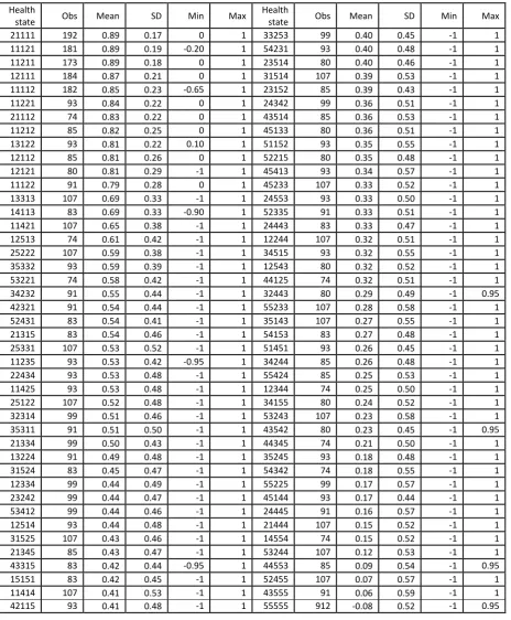
Table 1: Summary statistics for the 86 TTO health states
Health
state Obs Mean SD Min Max
Health
state Obs Mean SD Min Max
21111 192 0.89 0.17 0 1 33253 99 0.40 0.45 -1 1
11121 181 0.89 0.19 -0.20 1 54231 93 0.40 0.48 -1 1
11211 173 0.89 0.18 0 1 23514 80 0.40 0.46 -1 1
12111 184 0.87 0.21 0 1 31514 107 0.39 0.53 -1 1
11112 182 0.85 0.23 -0.65 1 23152 85 0.39 0.43 -1 1
11221 93 0.84 0.22 0 1 24342 99 0.36 0.51 -1 1
21112 74 0.83 0.22 0 1 43514 85 0.36 0.53 -1 1
11212 85 0.82 0.25 0 1 45133 80 0.36 0.51 -1 1
13122 93 0.81 0.22 0.10 1 51152 93 0.35 0.55 -1 1
12112 85 0.81 0.26 0 1 52215 80 0.35 0.48 -1 1
12121 80 0.81 0.29 -1 1 45413 93 0.34 0.57 -1 1
11122 91 0.79 0.28 0 1 45233 107 0.33 0.52 -1 1
13313 107 0.69 0.33 -1 1 24553 93 0.33 0.50 -1 1
14113 83 0.69 0.33 -0.90 1 52335 91 0.33 0.51 -1 1
11421 107 0.65 0.38 -1 1 24443 83 0.33 0.47 -1 1
12513 74 0.61 0.42 -1 1 12244 107 0.32 0.51 -1 1
25222 107 0.59 0.38 -1 1 34515 93 0.32 0.55 -1 1
35332 93 0.59 0.39 -1 1 12543 80 0.32 0.52 -1 1
53221 74 0.58 0.42 -1 1 44125 74 0.32 0.51 -1 1
34232 91 0.55 0.44 -1 1 32443 80 0.29 0.49 -1 0.95
42321 91 0.54 0.44 -1 1 55233 107 0.28 0.58 -1 1
52431 83 0.54 0.41 -1 1 35143 107 0.27 0.55 -1 1
21315 83 0.54 0.46 -1 1 54153 83 0.27 0.48 -1 1
25331 107 0.53 0.52 -1 1 51451 93 0.26 0.45 -1 1
11235 93 0.53 0.42 -0.95 1 34244 85 0.26 0.48 -1 1
22434 93 0.53 0.48 -1 1 55424 85 0.25 0.53 -1 1
11425 93 0.53 0.48 -1 1 12344 74 0.25 0.50 -1 1
25122 107 0.52 0.48 -1 1 34155 80 0.24 0.52 -1 1
32314 99 0.51 0.46 -1 1 53243 107 0.23 0.58 -1 1
35311 91 0.51 0.50 -1 1 43542 80 0.23 0.45 -1 0.95
21334 99 0.50 0.43 -1 1 44345 74 0.21 0.50 -1 1
13224 91 0.49 0.48 -1 1 35245 93 0.18 0.48 -1 1
31524 83 0.45 0.47 -1 1 54342 74 0.18 0.55 -1 1
12334 99 0.44 0.49 -1 1 55225 99 0.17 0.57 -1 1
23242 99 0.44 0.47 -1 1 45144 93 0.17 0.44 -1 1
53412 99 0.44 0.46 -1 1 24445 91 0.16 0.57 -1 1
12514 93 0.44 0.48 -1 1 21444 107 0.15 0.52 -1 1
31525 107 0.43 0.46 -1 1 14554 74 0.15 0.52 -1 1
21345 85 0.43 0.47 -1 1 53244 107 0.12 0.53 -1 1
43315 83 0.42 0.44 -0.95 1 44553 85 0.09 0.54 -1 0.95
15151 83 0.42 0.45 -1 1 52455 107 0.07 0.57 -1 1
11414 107 0.41 0.53 -1 1 43555 91 0.06 0.59 -1 1
42115 93 0.41 0.48 -1 1 55555 912 -0.08 0.52 -1 0.95
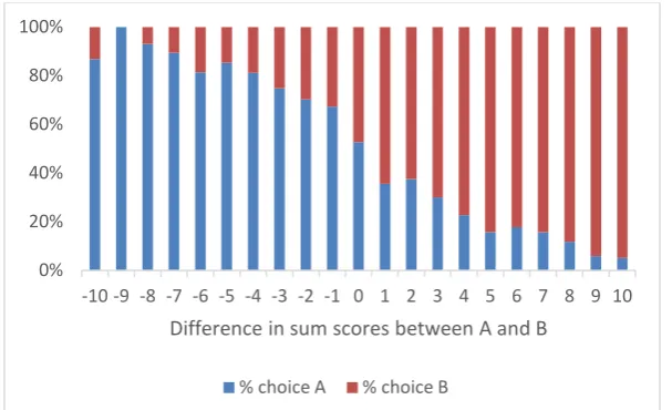
9 percentage of respondents who chose A, plotted against the differences in the sum score between the two options.
Figure 1: Percentage choosing A or B in the DCE tasks versus relative severities of A and B (N=996)
2.5
Interpretation of values at -1, 0 and 1.
2.5.1 Censoring at -1
When respondents completing a TTO task judge a health state – say “x” – to be worse than dead they may, at the extreme, prefer to die now than to live for 10 years in full health (the lead time) followed by 10 years in “x”. In that case the resultant value, given the variant of TTO used in the EQ-5D-5L valuation protocol, is -1. However, we cannot exclude the possibility that respondents who respond in this way would have traded more time in full health had they been presented with a longer lead time, in which case their value is lower than -1 (Devlin et al., 2013). As such, when a value of -1 is observed it can be interpreted as -1 or lower, which makes these values, in a statistical sense, “left censored” at -1.
2.5.2 Censoring at 0
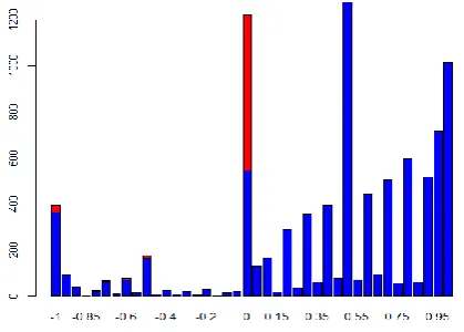
When the TTO data for each respondent were plotted against the predicted TTO values from the 10 parameter DCE tariff, we found that most respondents’ data followed a negative gradient as expected (i.e. valuing more severe health states lower than less severe health states). However, some respondents use zero as the minimum value more than once, including when valuing the worst health state 55555. This suggests that
-10 -9 -8 -7 -6 -5 -4 -3 -2 -1 0 1 2 3 4 5 6 7 8 9 10 0%
20% 40% 60% 80% 100%
Difference in sum scores between A and B
10 those respondents did not want to go below zero (i.e. do not believe there is such a thing as a health state so bad that experiencing it for 10 years would be worse than being dead). Consequently, these respondents do not distinguish between 55555 and other health states which are logically better (55555 is dominated by all other EQ-5D-5L health states), leading to a situation in which no value is attached to improvements from 55555 to less severe health states. With hindsight it was interpreted that when a respondent valued more than one health state (almost always including 55555) at zero that these values are not necessarily equal. This is captured by interpreting the observed zero values as being either zero or less than zero. In statistical terms, those zeros are interpreted as being “censored at zero”. This concerns 150 respondents and 595 observed zero values.
Further, a number of respondents valued 55555 at zero whilst valuing more than one other health state at less than zero. This is logically inconsistent. Either the values below zero should be higher, or the value of 55555 should be lower. We know the direction of the error but not the magnitude. We censored those negative values and associated zero values at zero. This concerns 27 individuals and 154 observations.
[image:12.595.84.294.487.637.2]Figure 2 shows the number of observations for each TTO value. The red bars show the number of observations censored at zero. In total we censored 749 observations (154 + 595 = 749) at zero.
Figure 2: Number of observations censored and not censored at zero against the TTO value
11
2.5.3 Censoring at 1
Some respondents gave relatively low values, e.g. 0.5 or 0, to the least severe states resulting in relatively large differences between the mean and the median value. For example, the mean and median for health state 11211 are 0.95 and 0.89 respectively. Respondents could make errors in the composite TTO tasks, defined as the deviation of the observed from the true TTO value. While one can make an error to the left and value this health state at 0, one cannot make an equivalent error to the right and score it at, say, 2. So, the error distribution is likely not to be normally distributed, which also explains why the mean and median are quite different. Now, imagine the TTO scale as viewed by respondents with 1 on the right and 0 towards the left. When valuing a given health state they may imagine the state, and look to place it on the TTO scale. If respondents make errors to the left, the state ends up with an observed value which is lower than the true value (and this observed value can be as low as -1). If respondents make errors to the right, the maximum value they can give is 1. Therefore, values at 1 could be considered as being either 1 or greater than 1 (i.e. ”right censored”). To censor TTO data at 1 might be considered arbitrary. However, to assume the errors follow a normal distribution is incorrect as the assumption denies the fact that the theoretical TTO values could exceed 1.
3.
Methods
Both TTO and DCE data can be used individually to produce a value set. We present results using DCE data, TTO data, and TTO/DCE data combinations.
Model parameter specification
3.1
Within each method, models were estimated with 5, 9, 10 and 20 parameters, with and without interaction terms, and with and without terms capturing some degree of decreasing marginal severity, corresponding with the “N3 term” used in the 3-level UK tariff (Dolan, 1997).
12 The 9 parameter model estimates one parameter per dimension and one parameter per level (4 levels + 5 dimensions = 9 parameters). In theory, the 5 dimension parameters could add up to one. To save the degrees of freedom, we actually estimate 4 dimension parameters rather than 5. Therefore, the 9 parameter model could be viewed as an 8 parameter model (4 levels + 4 dimensions = 8 parameters) with the additional dimension parameter constrained. The assumptions behind this model is that there is a linear relationship between the TTO values and the five dimensions. The impact of each level is the same across all five dimensions.
Unlike the 9 parameter model, the 10 parameter model estimates two parameters for level 5 (one for the mobility, self-care and usual activity dimensions where level 5 describes being “unable” to do a certain function; the other for the pain/discomfort and anxiety/depression dimensions where level 5 described having ”extreme” problems). As in the 9 parameter model, we estimate 4 dimension parameters. Therefore we actually estimate 9 parameters with one dimension parameter constrained instead of 10 parameters.
The 20 parameter model estimates four parameters for each dimension and one parameter per level, with the “no problems” level used as the baseline (4 levels x 5 dimensions = 20 parameters). This model allows the coefficients to differ between dimensions, and for the importance of each level of problems to differ between dimensions.
Below we use the 20 parameter model without interactions to illustrate our methods.
Modelling the discrete choice data
3.2
When considering the DCE data, respondents compare the utilities of two health states, i.e. Vijl and Vijr. The Vijl comes from individual i for health state presented on the left
hand side l within DCE pair j. We formulate the comparison in equation (1):
When assuming that the errors are normally distributed the parameters can be estimated by maximum likelihood as in a probit model. When assuming that the errors follow an extreme value distribution the parameters can be estimated by maximum likelihood as in a logistic regression. A constant term that is significantly different from zero suggests an overall preference for the health state appearing either on the left or on the right hand side. We use the logistic regression, as we assume that errors in
(1)
?
20 1 20 1 rj i k rj k k r ijr lj i k lj k k lijl
x
e
V
x
e
V
13 equation (1) may show extreme values. For instance, respondents could value severe health state as negative infinity.
Modelling the TTO data
3.3
When modelling the DCE data the parameters only have a relative value. It provides information on the relative preference of one health state over another. When using TTO data, the parameters can be interpreted as measuring a deviation from full health on a scale anchored at 1 (representing full health) and 0 (the value for dead). As with DCE we assume a value function that is linear between the value and the description of the health state. The specification is shown by equation (2).
𝑉𝑖𝑗 is the TTO value for health state j from respondent i. Parameters 𝛽𝑘reflect the real
decrement from full health. The error term 𝑒𝑖𝑗 measure the difference between an observed TTO value and the mean value. It captures random errors as well as differences of opinion between respondents about health states. In a linear regression analysis, the random error term is assumed to follow a normal distribution with mean of zero and constant variance. We follow this assumption but, as indicated above, there may be censoring at -1, 0 and 1.
Three further issues require consideration. First, it is observed that the variance of TTO values is larger for poorer health states than for better health states. This is due to a divergence in preferences regarding these states, but also increased respondent error. Second, there is the pseudo continuity of the data – only 41 unique values between -1 and 1 are available to respondents. Third, we limit the parameter space such that coefficients are always logically consistent.
Heteroskedasticity/heterogeneity
3.3.1
The variation of TTO values between more severe and less severe states means that the error terms in modelling the TTO data show heteroskedasticity. One explanation is that values for the mildest health states could sensibly be in a relative narrow range of 0.8 and 1 for example, whereas the sensible range of values for the more severe health states could be much larger, e.g. between -1 and 0.5. This is because respondents could use 1 as a baseline to value the mildest health states. However, for severe health states,
(2)
)
(
1
20 1 j i k j ik k ji
x
e
V
14 respondents apply their own scale and there is no baseline value to use. They can score any value between -1 to 1. The heteroskedasticity is captured by applying a linear relationship between the variance and the mean of the error terms per health state, adding two parameters to the model. A negative linear relationship between the mean and variance of the error terms indicate that the respondents use a smaller range of TTO values for mild health states than severe health states.
An alternative and probably more fundamental way of capturing the increasing variance in the error terms with the increasing level of severity in health states is to take into account the heterogeneity of respondents’ opinions. We observe that respondents effectively use different TTO scales, e.g. some respondents never give negative TTO values, some give both negative and positive TTO values, and some express “extreme” views about some health states. It is expected that respondents disagree more about severe health states than milder health states. The heterogeneity of TTO scales that respondents used could be explained by the disagreement about the value of dead between respondents. This is captured by introducing a parameter for disutility scale 𝛾, which may differ between respondents. The specification is reported by equation (3).
We investigate three assumptions of the distribution in 𝛾: (i) a normal distribution with mean 1 and a variance which needs to be estimated; (ii) a lognormal distribution with mean 1 and a variance which needs to be estimated; and (iii) a multinomial distribution with probability density on a number of discrete values. It is envisaged that the tail in the lognormal distribution may capture some respondents with extreme values. The multinomial model corresponds with the notion that there may be a number of latent groups, each having their own mean and variance. In our analysis, we experimented the number of probability density that equals to 2, 3 and 4. For normalisation, the mean value of 𝛾 for one of the three latent groups has value constrained to 1. Within this model, we also assume that there is heteroskedasticity which may be different per group.
Continuity of the TTO data
3.3.2
Given the study protocol (and the iteration used to arrive at a point of indifference– see Oppe et al., 2014), respondents can only give 41 distinct values. These range from -1 to 1 with steps of 0.05 between each distinct value. Apart from the two boundary values -1 and 1, for each observed TTO value x we assume that the true value lies within the range [x-0.025, x+0.025]. The value 0.025 is the mid-point of the gap between two
(3)
)
(
1
20 1 j i k j ik k i ji
x
e
V
15 neighbouring TTO values. For instance, when a respondent gives the value 0.5, the true value could be in a scale of 0.475 and 0.525 which are the midpoints of the nearest available values 0.45 and 0.55. More subtle rules to define the true scale for observed TTO values are possible. These rules depend on the process by which respondents arrive at their TTO values. In our case, the mid-point was considered an appropriate rule for defining the scales for observed values.
We analyse how the standard censored model changes when we treat TTO data as non-continuous (or interval censoring). The interval censoring triggers the question about how to censor TTO values at -1 and 1. When we observe a TTO value at 1, the true value could be in a scale of 0.975 and 1. Instead of censoring the TTO value at the top end of 1, we censored it at 0.975 when modelling the TTO data as non-continuous variable. The same analysis was applied to the bottom end. Therefore, we censored TTO data at -0.975 rather than -1 when modelling the TTO data as non-continuous.
Forcing consistency
3.3.3
The parameter for the “moderate” level is expected to be larger than that for “slight” and lower than that for “severe”, etc. However, when estimating the parameters freely, “logically inconsistent” estimates may be observed. It is hypothesized that while respondents may not always distinguish between different levels, they do not reverse the ordering. The estimated parameters should be logically consistent if respondents could correctly distinguish between different levels. The parameter space is used to reflect this. When defining our preferred models, this is captured by first estimating the parameters for the “slight” levels and then estimating those for the more severe levels by subsequently adding quadratic terms (which can only be zero or positive).
Hybrid model
3.4
16
Criterion for the ‘best’ model selection
3.5
With respect to models estimated from DCE data only, we choose the best model on the basis of the maximum likelihood statistics. We also use the maximum likelihood to compare the performance of TTO models that take account of the heteroskedasticity. For the models accounting for heterogeneity, we use the deviance information criterion (DIC) to compare performance. The best hybrid model with heteroskedasticity and best hybrid model with heterogeneity are compared using the DIC. The coefficient ordering and the face validity of the value range are also compared.
It should be noted that the “best” model is not necessarily expected to predict the mean observed values from the TTO data the best. That is because some observations are censored, and as a result the mean is not the best measure of central tendency. Furthermore, we use not only the TTO data but also the DCE data in the hybrid model, whereas observed values are available only from TTO data.
Sensitivity analyses
3.6
Four sensitivity analyses are conducted to check the robustness of the 20 parameter hybrid model results. Each analysis reveals the impact of one – potentially arbitrary – decision we made. The first sensitivity analysis checks the impact of exclusion criteria on the value set. We run the hybrid model without excluding any TTO observations from the data set (section 2.3). The second sensitivity analysis checks the impact of censoring the TTO data at -1, 0 and 1 (section 2.5).
17
4.
Results
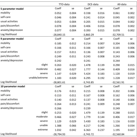
[image:19.595.70.547.236.712.2]The results for the 5, 9 and 10 parameter models for the DCE, TTO and combined datasets are reported in Table 2. The 5 parameter model offers a first impression of which dimensions get the highest weight, i.e. pain/discomfort followed by anxiety/depression. The DCE data indicate a higher weight for mobility than for usual activities and self-care, whereas the TTO data give approximately equal weights for mobility and usual activities.
Table 2: Estimates using the 5, 9 and 10 parameter models
TTO-data DCE-data All-data
5 parameter model Coeff se Coeff se Coeff se
mobility 0.052 0.004 0.338 0.016 0.061 0.002
self-care 0.046 0.004 0.241 0.014 0.045 0.002
usual activities 0.053 0.004 0.205 0.015 0.044 0.002
pain/discomfort 0.078 0.004 0.406 0.016 0.078 0.002
anxiety/depression 0.077 0.004 0.393 0.015 0.078 0.002
Log likelihood -28,840.15 -3,860.29 -32,709.51
9 parameter model Coeff se Coeff se Coeff se
mobility 0.185 0.012 0.214 0.007 0.204 0.006
self-care 0.166 0.011 0.166 0.007 0.165 0.006
usual activities 0.157 0.011 0.136 0.007 0.143 0.006
pain/discomfort 0.249 0.011 0.243 0.008 0.243 0.006
anxiety/depression 0.242 0.241 0.244
slight 0.263 0.020 1.478 0.139 0.290 0.015
moderate 0.482 0.027 1.777 0.144 0.409 0.016
severe 1.147 0.029 5.424 0.183 1.120 0.019
unable/extreme 1.183 0.020 6.295 0.192 1.228 0.017
Log likelihood -28,801.61 -3,743.85 -32,561.91
10 parameter model Coeff se Coeff se Coeff se
mobility 0.176 0.011 0.215 0.008 0.202 0.006
self-care 0.153 0.011 0.167 0.008 0.162 0.006
usual activities 0.140 0.012 0.137 0.008 0.140 0.006
pain/discomfort 0.264 0.013 0.241 0.009 0.248 0.007
anxiety/depression 0.266 0.239 0.249
slight 0.253 0.020 1.479 0.139 0.288 0.015
moderate 0.466 0.027 1.779 0.144 0.406 0.017
severe 1.129 0.029 5.430 0.183 1.116 0.020
unable 1.388 0.066 6.217 0.246 1.266 0.034
extreme 1.032 0.042 6.363 0.237 1.195 0.027
18 The 9 parameter model offers a significant improvement according to the likelihood ratio test and we observe – in both the DCE and the TTO data – that the decrement from slight to moderate and from severe to unable/extreme are much smaller than the decrement from moderate to severe. Having different parameters for level 5 based on descriptor improves the TTO model but not the DCE model. The parameter for unable is larger than that for severe in all three 10 parameter models but the parameter for extreme is not in the TTO model, which suggests an “inconsistency”.
19
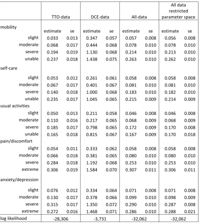
Table 3: 20 parameters model with and without restriction
TTO-data DCE-data All-data
All data restricted parameter space
mobility
estimate se estimate se estimate se estimate se
slight 0.033 0.013 0.347 0.057 0.057 0.008 0.056 0.008
moderate 0.068 0.017 0.444 0.068 0.078 0.010 0.078 0.010
severe 0.194 0.019 1.130 0.068 0.214 0.010 0.213 0.010
unable 0.237 0.018 1.438 0.075 0.263 0.010 0.262 0.010
self-care
slight 0.053 0.012 0.261 0.061 0.058 0.008 0.058 0.008
moderate 0.067 0.017 0.401 0.067 0.081 0.010 0.081 0.010
severe 0.140 0.018 1.000 0.068 0.183 0.010 0.182 0.010
unable 0.235 0.017 1.045 0.065 0.215 0.009 0.214 0.009
usual activities
slight 0.050 0.013 0.211 0.058 0.046 0.008 0.046 0.008
moderate 0.110 0.016 0.217 0.065 0.068 0.009 0.068 0.009
severe 0.185 0.017 0.798 0.065 0.172 0.009 0.170 0.008
unable 0.165 0.018 0.815 0.067 0.167 0.009 0.170 0.018
pain/discomfort
slight 0.054 0.011 0.333 0.062 0.058 0.008 0.058 0.008
moderate 0.066 0.018 0.381 0.065 0.080 0.010 0.080 0.010
severe 0.284 0.018 1.192 0.068 0.253 0.010 0.253 0.010
extreme 0.306 0.019 1.584 0.070 0.307 0.011 0.306 0.011
anxiety/depression
slight 0.076 0.012 0.334 0.064 0.071 0.008 0.071 0.008
moderate 0.130 0.017 0.378 0.066 0.099 0.010 0.098 0.009
severe 0.315 0.017 1.350 0.072 0.290 0.010 0.287 0.008
extreme 0.272 0.016 1.468 0.071 0.286 0.010 0.288 0.021
log likelihood -28,306 -3,731 -32,062 -32,062
20
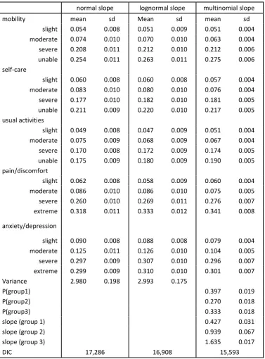
Table 4: Estimates using all data 20 parameter model with different slope distributions
normal slope lognormal slope multinomial slope
mobility mean sd Mean sd mean sd
slight 0.054 0.008 0.051 0.009 0.051 0.004
moderate 0.074 0.010 0.070 0.010 0.063 0.004
severe 0.208 0.011 0.212 0.010 0.212 0.006
unable 0.254 0.011 0.263 0.011 0.275 0.006
self-care
slight 0.060 0.008 0.060 0.008 0.057 0.004
moderate 0.083 0.010 0.080 0.010 0.076 0.004
severe 0.177 0.010 0.182 0.010 0.181 0.005
unable 0.211 0.009 0.220 0.010 0.217 0.005
usual activities
slight 0.049 0.008 0.047 0.009 0.051 0.004
moderate 0.075 0.009 0.068 0.009 0.067 0.004
severe 0.170 0.008 0.172 0.009 0.174 0.005
unable 0.175 0.009 0.180 0.009 0.190 0.005
pain/discomfort
slight 0.062 0.008 0.058 0.009 0.060 0.004
moderate 0.086 0.010 0.086 0.010 0.075 0.005
severe 0.260 0.010 0.269 0.011 0.276 0.007
extreme 0.318 0.011 0.333 0.012 0.341 0.008
anxiety/depression
slight 0.090 0.008 0.088 0.008 0.079 0.004
moderate 0.125 0.011 0.126 0.010 0.104 0.005
severe 0.297 0.009 0.307 0.010 0.296 0.007
extreme 0.299 0.009 0.310 0.010 0.301 0.007
Variance 2.980 0.198 2.993 0.175
P(group1) 0.397 0.019
P(group2) 0.270 0.018
P(group3) 0.333 0.018
slope (group 1) 0.427 0.031
slope (group 2) 0.939 0.067
slope (group 3) 1.635 0.017
DIC 17,286 16,908 15,593
In Table 4, we report the results for 3 latent groups in the multinomial slope model. The multinomial slope model divides all respondents into 3 latent groups which is based on the similarity of their slopes. Increasing the number of groups from 3 to 4 in the multinomial model did not improve the estimates.
21 indicates that the three random slope models, which reported in Table 4, offer an improvement. The lowest DIC is achieved in the all-data-20-parameter multinomial slope model, i.e. 15,593. This model is therefore considered as the best performing model for data from the EQ-5D-5L value set for England project. This includes a further improvement that is achieved by capturing heteroskedasticity using two parameters per group to model the dependency between the variance per health state and the mean per health state.
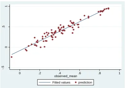
Figure 3 illustrates the predicted utilities and observed TTO for the 4 all-data-20 parameter models. Predicted utilities for the 86 health states in Figure 3.1 used all data restricted parameter space model (Table 3). Predicted utilities in Figure 3.2 used normal slope model (Table 4). Predicted utilities in Figure 3.3 used lognormal slope model (Table 4). Predicted utilities in Figure 3.4 used multinomial slope model (Table 4).
3.1: All data restricted parameter space model 3.2: Normal slope model
3.3: Lognormal slope model 3.4: Multinomial slope model
When comparing the estimates of the least severe and worst health states from all models we find that the prediction of 11211 (slight problems in usual activities and no problems on any other dimension) and 21111 (slight problems in mobility and no problems on any other dimension) score above 0.95. This is higher than the mean
-.
5
0
.5
1
0 .2 .4 .6 .8 1
observed_mean Fitted values prediction
-.
5
0
.5
1
0 .2 .4 .6 .8 1
observed_mean Fitted values prediction
-.
5
0
.5
1
0 .2 .4 .6 .8 1
observed_mean Fitted values prediction
-.
5
0
.5
1
0 .2 .4 .6 .8 1
[image:23.595.312.515.357.499.2] [image:23.595.73.278.360.501.2]22 observed values of 0.89, which we believe to be biased due to the asymmetry of the error distribution. The score for 55555 varies across models: -0.240 for the model without heterogeneity, -0.257 for the normal slope model, -0.306 for the lognormal slope model, and -0.281 for the multinomial slope model. The lower values reflect the potential of the latter two models to capture more extreme values.
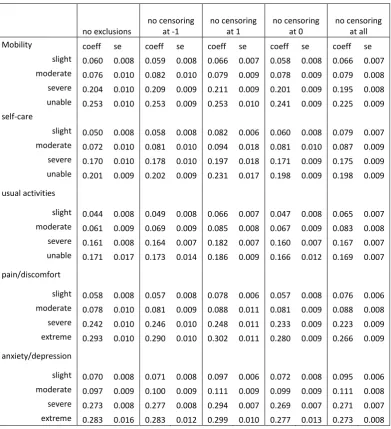
We made a number of decisions about how to interpret the data, and these were subjected to sensitivity analysis. Table 5 presents results of the 20 parameter hybrid model if we hadn’t made those decisions. Column 2 shows the results if we had not applied any exclusion criteria to the raw data set. Hence, there are 996 individuals included in the analysis. Health state 11211 (i.e., slight problem with usual activities and no problem in any other four dimensions) has the highest value of 0.956. The lowest value is reported as -0.201 for health state 55555. Columns 3 to 6 reports four sets of results from the sensitivity analysis without censoring: column 3 shows the results without censoring at -1; column 4 without censoring at 1; column 5 without censoring at 0; and column 6 shows the results if there was no censoring at all. Calculations from the four sets of results in columns 3 to 6 all suggest that health state 11211 has the highest value. Only for results that are reported in column 4, i.e. without censoring at 1, suggest that health states 21111 and 11211 have the same value. The value for health state 11211 is 0.951 if the TTO data are not left censored at -1; 0.934 if TTO data are not right censored at 1; 0.953 if the TTO data are not censored at zero; and 0.935 if the TTO data are not censored at all. The lowest value is for health state 55555. It is reported as -0.201 if the TTO data are not left censored as -1; -0.271 if the TTO data are not right censored at 1; -0.162 if the TTO data are not censored at zero; and -0.131 if the TTO data are not censored at all.
23
Table 5. Effects of different interpretations of the hybrid model data
no exclusions
no censoring at -1
no censoring at 1
no censoring at 0
no censoring at all
Mobility coeff se coeff se coeff se coeff se coeff se
slight 0.060 0.008 0.059 0.008 0.066 0.007 0.058 0.008 0.066 0.007 moderate 0.076 0.010 0.082 0.010 0.079 0.009 0.078 0.009 0.079 0.008 severe 0.204 0.010 0.209 0.009 0.211 0.009 0.201 0.009 0.195 0.008 unable 0.253 0.010 0.253 0.009 0.253 0.010 0.241 0.009 0.225 0.009
self-care
slight 0.050 0.008 0.058 0.008 0.082 0.006 0.060 0.008 0.079 0.007 moderate 0.072 0.010 0.081 0.010 0.094 0.018 0.081 0.010 0.087 0.009 severe 0.170 0.010 0.178 0.010 0.197 0.018 0.171 0.009 0.175 0.009 unable 0.201 0.009 0.202 0.009 0.231 0.017 0.198 0.009 0.198 0.009
usual activities
slight 0.044 0.008 0.049 0.008 0.066 0.007 0.047 0.008 0.065 0.007 moderate 0.061 0.009 0.069 0.009 0.085 0.008 0.067 0.009 0.083 0.008 severe 0.161 0.008 0.164 0.007 0.182 0.007 0.160 0.007 0.167 0.007 unable 0.171 0.017 0.173 0.014 0.186 0.009 0.166 0.012 0.169 0.007
pain/discomfort
slight 0.058 0.008 0.057 0.008 0.078 0.006 0.057 0.008 0.076 0.006 moderate 0.078 0.010 0.081 0.009 0.088 0.011 0.081 0.009 0.088 0.008 severe 0.242 0.010 0.246 0.010 0.248 0.011 0.233 0.009 0.223 0.009 extreme 0.293 0.010 0.290 0.010 0.302 0.011 0.280 0.009 0.266 0.009
anxiety/depression
24
5.
Discussion and Conclusions
The primary aim of this study was to adapt the modelling methods that were used to produce value sets for EQ-5D which correspond to the newly designed elicitation method, comprising a different type of TTO and with the addition of DCE. Additionally, a number of developments in the modelling approaches were made, compared to earlier approaches, which bring the models closer to the nature of the data.
The new study design combined TTO data with DCE data. The lead time TTO approach was used which meant that the minimum value respondents could score was -1 without information about whether that value or a lower value was respondents’ genuine preference. The data were seen as censored and the true value were not observed. Therefore, an assumption should be made for the (left tail of the) distribution of the TTO data. We experimented model that assumed a normal distribution with errors and accounting for the heteroskedasticity. And when experimenting models that account for the heterogeneity of respondents, the assumption of normal distribution for errors is still applied. With the heterogeneity models, we experimented the assumptions of slope for disutility in health with a normal distribution, lognormal distribution and a multinomial distribution. Our results suggest that the assumptions of distributions affects the value of poor health states, as well as the predicted TTO values in particular for values where the real data points in our data set is limited. In contrast, the respondents in the Measurement and Valuation of Health (MVH) study could score TTO value as low as -39. In order to minimise the effect of extreme values, a decision was taken to rescale the TTO values to a range of [-1, 1]. It suggests that the extreme negative values in TTO are possible. Indeed, some respondents may not want to end – coûte que coûte – in certain health states and their values may have great impact on the averages. The solution may be to use medians or to exclude extremes at both the lower and upper end of the scale.
25 Another aspect which has been given attention is the fact that the TTO data are not really continuous, as respondents can only give 41 distinct values. Therefore, when a respondent scores 0.9, instead of 0.85 or 0.95, it might indicate that the true value locates in a scale between 0.925 and 0.975. Furthermore, respondents have a digit preference. They are more likely to end up with 0.1, than 0.05 or 0.15 for example. We used the simple correction for our heteroskedasticity model by censoring the upper end of TTO value at 0.975 rather than 1. In together with the left censoring at -0.975, this censoring exercise is also applied to the heterogeneity models, which are estimated without defining intervals for other TTO values. This characteristic of the TTO data was not recognised by the MVH study, although respondents could score more (80) unique values.
With the addition of the DCE data, we choose to combine the information into a single likelihood function and assuming that the underlying preference function which dictates the answers to the DCE comparisons also dictates the answers to the TTO questions. It should be noted that the DCE data is under the assumption that errors, or differences of opinion, are normally distributed. It might be true for errors, however it is unlikely to be true for differences in opinion. In the multinomial model, we identify a group of respondents who always score positive values, a group of respondents who score both positive and negative values, as well as a group of respondents with extreme values. The DCE data, in this design, are not rich enough to pick up such clear differences. Therefore, estimations that are based on DCE data only might be criticised by such an assumption with the error distributions. However, different from some of the findings of modelling TTO data only, all parameters in the DCE modelling results were logically consistent. Also the results from the DCE models show the general structure of the value set, i.e. with small steps between slight and moderate levels, big steps between moderate and severe level, and again small steps between severe and extreme/unable levels. It is observed that the TTO data and the DCE data lead to different parameter estimates. The TTO data seems to be the closest to the decision making context where trade-offs need to be made between length of life and quality of life. One may criticize the error distribution of the DCE model, but this may also apply to the TTO data.
26 to be made and feel that this is a consequence of having an outside agency doing the interviews with strict guidance not to interfere, even when one might think that this is needed.
Another aspect which may need further justification is that we formulated rather vague prior distributions which guaranteed that the differences between the levels were positive. Indeed when estimated without constraint, the TTO data may suggest that the severe level (level 4) is worse than extreme level (level 5) in the anxiety/depression dimension. We don’t find this in the DCE data, and one explanation for this may relate to the selection of the 86 health states in the TTO exercise. Additionally, we find justification of our priors by referring to the research that underlying the choice of the labels in the EQ-5D-5L (Luo et al., 2015).
27
REFERENCES
Brazier, J., Ratcliffe, J., Salomon, J.A. and Tsuchiya, A., 2007. Measuring and valuing health benefits for economic evaluation. Oxford: Oxford University Press.
Devlin, N., Shah, K., Feng, Y., Mulhern, B. and van Hout, B., 2015. Valuing health-related quality of life: an EQ-5D-5L value set for England. OHE Research Paper. London: Office of Health Economics.
Devlin, N. and Buckingham, K., 2013. What is the normative bias for selecting the measure of average’ preferences to use in social choices? Paper presented at the 30th
EuroQol Scientific Plenary. Montreal, Canada. 12-13 September.
Devlin, N., Buckingham, K., Shah, K., Tsuchiya, A., Tilling, C., Wilkinson, G. and van Hout, B., 2012. A comparison of alternative variants of the lead and lag time TTO. Health Economics, 22(5), pp.517-532
Devlin, N. and Krabbe, P., 2013. The development of new research methods for the valuation of EQ-5D-5L. European Journal of Health Economics, 14(Suppl 1), pp.S1–S3. Dolan, P., 1997. Modeling valuations for EuroQol health states. Medical Care, 35(11), pp.1095-1108.
Herdman, M., Gudex, C., Lloyd, A., Janssen, M.F., Kind, P., Parkin, D., Bonsel, G. and Badia, X., 2011. Development and preliminary testing of the new five-level version of EQ-5D (EQ-5D-5L). Qualife of Life Research, 20(10), pp.1727-1736.
Janssen, B., Oppe, M., Versteegh, M. and Stolk, E., 2013. Introducing the composite TTO: a test of feasibility and face validity. European Journal of Health Economics, 14, pp.5-13.
Luo, N., Wang, Y., How, C.H., Tay, E.G., Thumboo, J. and Herdman, M., 2015.
Interpretation and use of the 5-level EQ-5D response labels varied with survey language among Asians in Singapore. Journal of Clinical Epidemiology, 68(10), pp.1195-1204. Oppe, M., Devlin, N. J., van Hout, B., Krabbe, P.F. and de Charro, F., 2014. A program of methodological research to arrive at the new international EQ-5D-5L valuation protocol.
Value in Health, 17, pp.445-453.
Pullenayegum, E. and Xie, F., 2013. Scoring the 5-Level EQ-5D: Can Latent Utilities Derived from a Discrete Choice Model Be Transformed to Health Utilities Derived from Time Tradeoff Tasks? Medical Decision Making, 33(4), pp.567-578.
Rowen, D., Brazier, J. and van Hout, B., 2014. A Comparison of Methods for Converting DCE Values onto the Full Health-Dead QALY Scale. Medical Decision Making, 35(3), pp.328-340.