The effect of environmental stochasticity on species richness in neutral communities

Matan Danino1, Nadav M. Shnerb1, Sandro Azaele2, William E. Kunin3 and David A. Kessler1 1 _{Department of Physics, Bar-Ilan University, Ramat-Gan IL52900, Israel}

2

Department of Applied Mathematics, School of Mathematics, University of Leeds, Leeds, UK 3

School of Biology, University of Leeds, Leeds, UK.

Environmental stochasticity is known to be a destabilizing factor, increasing abundance fluctua-tions and extinction rates of populafluctua-tions. However, the stability of a community may benefit from the differential response of species to environmental variations due to the storage effect. This paper provides a systematic and comprehensive discussion of these two contradicting tendencies, using the metacommunity version of the recently proposed time-average neutral model of biodiversity which incorporates environmental stochasticity and demographic noise and allows for extinction and speciation. We show that the incorporation of demographic noise into the model is essential to its applicability, yielding realistic behavior of the system when fitness variations are relatively weak. The dependence of species richness on the strength of environmental stochasticity changes sign when the correlation time of the environmental variations increases. This transition marks the point at which the storage effect no longer succeeds in stabilizing the community.

Keywords: Community dynamics; Environmental stochasticity; Storage effect; Neutral theory.

I. INTRODUCTION

One of the biggest puzzles in community ecology is the persistence of high-diversity assemblages. The competitive exclusion principle [1, 2] predicts that the number of species coexisting in a local community should be fewer than or equal to the number of limiting resources, in apparent contrast with the dozens and hundreds of locally coexisting species of freshwater plankton [3, 4], trees in tropical forests [5] and coral reef species [6]. This problem has received considerable attention in recent decades, with many mechanisms suggested to circumvent the mathematical constraints embodied in the exclusion principle and many works that try to provide empirical support to these theories [7–9].

Within this framework, neutral theories, and in particular the neutral theory of biodiversity (NTB) suggested by Hubbell [10–12], play an important role. Under neutral dynamics all individuals are considered as having the same fitness, and abundance variations are the result of demographic noise alone. The number of individuals belonging to each species varies randomly within the limit imposed by the overall size of the community, with most populations eventually drifting to extinction. However, the neutral turnover rate is very slow, and diversity is maintained due to the introduction of new species into the system, either via speciation (in the metacommunity) or by migration (in a local community).

The slow turnover dynamics in the neutral model is not only an advantage, it is also a disadvantage, and has triggered one of the main lines of criticism directed at the neutral model. It turns out that pure ecological drift is far too slow to account for both the observed short-term fluctuations and the long term dynamics [13–18]. For example, the abundance of the most common species in the Barro-Colorado Island Smithsonian 50 ha plot has decreased from 40000 to 30000 individuals (>1cmdbh) during about half of a generation, while under pure demographic noise one expects variations of order√N ∼200 within a whole generation. The abundance of the most common species in the Amazon basin is about 109 _{individuals [5]. Under neutral dynamics, this is the age (in generations) of that species,} and since the generation time for tropical trees is about 50 years, this timescale (5·1010y) is longer than the age of the universe [13–15]. Recent work ([19], see also [20]) shows that species ages in neutral models are in fact lower than these early estimates by about two orders of magnitude, however these ages are still too high to be realistic.

Motivated by these difficulties, recent works [21, 22] have pointed towards a generalized neutral theory that will include both demographic andenvironmental stochasticity. Basically, this new model accepts the equivalence prin-ciple, but assumes that the fitness of all species is equal when averaged over time, while at any instant some species have higher fitness than the others due to temporal variations in parameters such as temperature, precipitation etc. Accordingly, all species are symmetric and abundance variations are driven by fluctuations [23]. The abil-ity of this time-averaged neutral theory of biodiversabil-ity (TNTB) to explain different empirical patterns, including species abundance distributions, temporal fluctuations statistics and the growth in system dissimilarity over time, was demonstrated in [21].

the community, fluctuates in time. This differential response of species, when superimposed on buffered population growth and covariance between environment relative probability and competition [25] was shown to stabilize the system. Chesson and Warner showed how rare species, when compared with common species, have fewer per-capita losses when their fitness is low and more gains when their fitness is high. Accordingly, the population of rare species increases (their average growth rate is positive just because their relative abundance is low) and the system supports a stable equilibrium: species’ abundance fluctuates, but is attracted to a finite value by a restoring force.

Hubbell’s NTB, which takes into account demographic noise and speciation but with no environmental noise, provides us with one set of predictions for the patterns characterizing a community, such as species abundance distri-bution and species richness. The Chesson-Warner lottery game, taking into account only environmental stochasticity (without demographic noise or speciation) suggests another set. What happens under the general model of TNTB, where all these elements play a role? What patterns does it predict, and how do they depend on the strength of the storage effect? In [21] the TNTB was presented in the context of a mainland-island model and simulated island dynamics were compared with data from the Barro-Colorado Island (BCI) plot. Here we aim at understanding the metacommunity dynamics of the TNTB and to explain its relationships with both NTB and the lottery game.

To do that, we first revisit the storage effect, using the original Chesson-Warner model. In section II we consider the storage effect for two species, emphasizing the transition it shows from a balanced system, where the abundance of both species fluctuates around one half of the community, and an imbalanced state, with one rare and one frequent species. A deeper analysis of the equilibrium distribution poses a conceptual problem, namely that the result is independent of the amplitude of the environmental variations. This problem is discussed in section III, and indicates the need to incorporate demographic stochasticity into the model. Before doing that, in section IV we consider the original lottery game for communities with many species and discuss its applicability to empirical systems. Finally in section V the TNTB model, in which environmental variations, demographic stochasticity and speciation affect the community, is analyzed. Conclusions are presented in the last section.

II. A LOTTERY GAME FOR TWO SPECIES

In this section we study the simplest case, the storage effect in a community with two species playing the lottery game. Since we are ultimately interested in the TNTB, we assume that the fitness of both species is equal when averaged over time (species are equivalent). Note that the scope of the storage effect is wider, and it may stabilize a community even when the average fitness is different; we will return to this point in the discussion section.

To provide an intuitive numerical example, let us consider an extremely simple game. Imagine a forest with 100 trees,NA of species A andNB= 100−NA of species B. For simplicity we assume that there is no spatial structure, seeds and seedlings of both species are all around the forest, with relative frequencies that reflect the relative abundance of adult trees. During every year 20% of the trees are selected at random, independent of their species affiliation, to die (so that the generation time is five years). The gaps that remain after the trees’ death are filled by seedlings, where the chance of each seedling to capture the vacancy depends of its relative fitness, with the fitness varying in time. To have equivalent species the temporal fitness is taken to be an independent and identically distributed (i.i.d.) variables, so the chance of a particular species to be the fitter of the two in a certain year is 1/2. Under an extreme, “winner takes all” scenario, the fittest species of a given year captures all the 20 empty slots.

Now let us follow the dynamics. Consider the case where, at the beginning of a certain year,NA= 20 andNB= 80. After the death step,NA= 16 andNB = 64 (this is an average, since trees are picked to die at random, but for our purpose it is sufficient to trace the average). Now there are two options: if the winner of this year is species A, the year ends withNA= 36, NB= 64, while if the fittest species isB, the outcome will beNA= 16, NB= 84. One can easily see that the gain ofA when it wins, 16, is higher than the potential gain ofB, which increases its population only by four individuals when it wins. By the same token the losses of A when it is the inferior species are smaller then the losses ofB in the parallel situation.

While this example is misleading in several respects (in particular the unrealistic winner takes all assumption strongly affects the results), it still provides the basic intuition: although the average fitness of both species is the same, environmental variations provide benefit to the rarer one, as the opportunities for the rare species (when it wins) are greater than those of a common species and its risks (when it loses) are less. Accordingly, an effective stabilizing force acts against any deviation from the 50−50 partition.

Having established this intuition, let us turn to the original two-species model as presented in [24]. In this model there is no demographic noise, so the absolute number of individuals has no importance. Accordingly, the variables are species relative fractions. For two species, these arex1 and 1−x1.

species’ fitness. Accordingly the abundance of the two species after these steps, death and recruitment, is given by,

xt+1₁ =xt₁(1−δ) +δ f t 1xt1 ft

1xt1+f22xt2

xt+1₂ =xt₂(1−δ) +δ f t 2xt2 ft

1x t 1+f

t 2x

t 2

(1)

wheref_it>0 is the fitness of thei-th species during thet-th step. For two species system one can replacex2by 1−x1 to get a single recursion equation,

xt+1₁ =xt₁(1−δ) + δf t 1xt1 ft

1x t 1+f

t 2(1−x

t 1)

.

When the fitness is fixed in time, the fittest species will win the game and the abundance of the inferior species decreases monotonically towards zero. Chesson discovered that, when the fitness fluctuates in time, it stabilizes the populations. As mentioned above, to extend the neutral theory we require the long-term average off1 andf2 to be equal.

Two parameters are needed to characterize environmental stochasticity: its strength and its duration (correlation time).

1. The strength of the environmental stochasticity,σ2

E manifests itself in the spread of the fitness parameters fi. Without loss of generality one may take

fi=eγi, (2)

where the parameter γi is an independent and identically distributed (iid) variable picked from a distribution (say, a Gaussian or a uniform distribution) with zero mean and varianceσ2

E. IfσE2 = 0 thenfi≡1, all species have the same fitness and the dynamics stops,xt+1_i =xt_i. The largerσ_E2, the stronger the fitness variability.

2.δ is thecorrelation time of the environmental noise, measured in units of generations (see also the description of our agent-based simulation of the model in Appendix B). Our analysis of Eqs. (1) is based on the assumption that the fitnessfi is picked at random every elementary timestep, i.e., betweentand t+ 1 and so on. Within this period a fraction δ of the individuals die. To give a concrete example, in [21] the correlation time of the environmental stochasticity in the Barro-Colorado Island plot was found to be about 10 years, while the generation time is about 50y. To model this dynamics using Eqs. (1) one may takeδ= 1/5, meaning that the replacement of 1/5 of the trees takes place under (more or less) the same fitness regime.

In [26], Hatfield and Chesson showed how to map the discrete time equations (1) to a Fokker-Planck equation for P(x1), the probability that the relative abundance of species number 1 isx1,

∂P(x1, t)

∂t =δσ

2 E

_∂

∂x1

[x1(1−x1)(x1−1/2)P(x1, t)] +δ ∂2 ∂x2

1

x2₁(1−x1)2P(x1, t)

. (3)

We provide our own derivation of (3) from (1) in Appendix A. The steady-state solution can be seen to be,

Peq(x1) =C[x1(1−x1)]

1

δ−2_{, (4)}

whereC= Γ(2/δ−2)/Γ2(1/δ−1).

0 0.2 0.4 0.6 0.8 1 0

0.5 1 1.5 2 2.5 3 3.5 4

x

P

q

(

x

)

δ=0.1

δ=0.3

δ=0.5

δ=0.6

δ=0.7

FIG. 1: The equilibrium probability distribution function,Peq(x), given by Eq. (4), is plotted againstxfor different values

ofδ (see legend). Forδ <1/2 the distribution peaks around the symmetric point 0.5, and the peak becomes sharper whenδ decreases (still the decay is slower than exponential). Atδc= 1/2 the distribution is flat, and for smaller values ofδit develops

two peaks close to the extinction and the fixation points and a valley in the middle. The distribution is normalizable as long as δ <1. However, had the dynamics of Eq. (1) allowed an absorbing state (e.g., if one consider any fractionxsmaller thanxmin

as the state with no individual) the chance of extinction in case ofδ1/2 would have been much smaller than the chance if δ >1/2. As discussed in the main text, the pdfs shown here are independent ofσ2

E.

The net result is determined by the ratio between these terms, i.e., byδ, as illustrated in Figure 1: forδ <1/2 the deterministic term wins, leading to a distribution with a single maximum at 1/2, meaning that at any instant of time the community is likely to be well balanced, with both species represented by roughly the same number of individuals. Forδ >1/2, on the other hand,Peq is convex, with probability mass concentrated near the edges at zero and one. In this case the community is unbalanced, (almost) any snapshot picture of the community reveals strong dominance of one species, although the equivalence ensures that the time average fraction of each species is around 1/2.

The distribution peak forδ <1/2 resembles the Gaussian or exponential peak one finds when the system supports a deterministic stable equilibrium (an attractive fixed point of a nonlinear system), but this similarity is slightly misleading. The decay of Peq towards the edges is described by a power-law, not by an exponential or a Gaussian. This happens since the fixed point at 1/2 is noise induced in the first place.

The second key feature of Eq. (4) is that it has been derived from Eq. (1) by expanding it to the leading order in the fitness differences, so the emerging Peq has to beindependent ofσ2E (see Appendix A for more details). This approximation becomes better and better as σ2_E decreases; accordingly, the storage effect appears to stabilize the two-species community even for vanishingly small values ofσ2

E. The amplitude of fitness variations only sets the time scale, such that the time needed for the system to reach the equilibrium distribution scales like 1/σ2

E and diverges when the environmental noise vanishes, butPeq itself stays the same. In the next section we discuss the conceptual difficulties associated with this outcome.

For the sake of completeness we note that the storage effect acts to destabilize the system when the environmental stochasticity acts on mortality rather than on fecundity. One may realize that easily by repeating the “loser loses all” version of the numerical example above, where the low fitness species suffers all the mortalities but the recruitment depends on abundance and is independent of fitness. Under such a scenario the rarer species has more to lose than the commoner one, as a the fixed number of deaths would represent a larger share of its population [26].

III. STORAGE EFFECT AND DEMOGRAPHIC STOCHASTICITY: A CONCEPTUAL DISCUSSION

The results presented in the last section, and in particular the properties ofPeq, suggest that this classical model of the storage effect, with pure environmental noise, is incomplete and leads inevitably to a conceptual breakdown. In this section these difficulties are presented, and the inclusion of demographic stochasticity into the model is suggested as a possible (and plausible) solution.

As seen above, Peq depends only onδ, the correlation time of environmental variations, and not on their strength σ2

E(as long as higher orders inσ 2

that govern the lottery game, such processes have the ability to induce stability in the long run sinceδ→0 and the amplitude of fitness fluctuations is irrelevant.

Clearly, a reasonable model should yieldPeqthat depends onσ2E. It is highly implausible that infinitesimal changes in wind direction or in temperature play an essential role in stabilizing natural communities, no matter how much time the system is allowed to relax. A lower cutoff below which environmental variations are negligible has to be introduced. For example, one may suggest that the minimal correlation time that the model has to take into account is the time between two consecutive deaths of individuals, since all the events that affect the fitness of species between two deaths are integrated to determine the success probability of every seedling competing to replace a dead tree. By doing that one already introduces the discreteness of individuals into the model. Demographic stochasticity, which is the endogenous noise associated with the discreteness of the birth-death process, provides the natural mathematical tool to deal with these aspects of reality. Quantifying the strength of demographic noise by the parameter σ_D2 (the value of this parameter is discussed below), we expect that the equilibrium distribution (4) should be obtained, from a general theory with demographic fluctuations, in the limit σ2

D/σ2E → 0, but for any finite demographic noise the ratio betweenσ2

E andσ2Dshould enter the expression forPeq.

Another aspect of the result (4), which also provides a hint about the importance of discreteness, is the transition between the single peak, balanced distribution at small values of δ and the imbalanced distribution at large δ. Mathematically speaking, as long as the distribution is normalizable the solution is legitimate, so the theory holds for allδ <1 and breaks down only whenδ= 1, wherePeq diverges likex−1 at the edges. However in practice, when the number of individuals has to be an integer, this formal approach may be misleading. If the overall size of the community isJ individuals, the casex <1/Jshould be considered as extinction. No matter whatδis, in the long run one of the two species inevitably goes extinct and the system reaches fixation. This feature is missing in the lottery game, where all positive values are allowed forx.

Accordingly, the stability of the system depends not only on the shape of Peq, but also on the rate at which the abundance of a single species scans through all the values ofxand reaches values below 1/J, a feature that depends strongly onσ2

E[28]. Even ifPeq(x) is very small forxclose to zero in the regimeδ <1/2, under strong environmental noise the species’ abundance samples the whole phase space on relatively short timescales, leading to fast fixation. As we shall see, since the decay ofPeq at the edges is a power law at best, one cannot neglect extinctions even when J is large.

Demographic stochasticity has two aspects. First, it opens the possibility of extinction by allowing a species to reach an absorbing state at zero concentration. Second, it provides another source of noise, which scales like the square root of the population size, as opposed to the linear scaling that characterizes environmental stochasticity [17, 29]. These two aspects of demographic noise are of importance to the study of the storage effect, and they manifest themselves in TNTB. However, before considering TNTB we would like to study the relevance of the storage effect, in its traditional form with only environmental stochasticity, to the statistics of high-diversity assemblages.

IV. THE LOTTERY GAME FOR MANY SPECIES

The applicability of the storage effect as a possible explanation for an empirical system with tens and hundreds of species was considered by Hubbell in [30], during the introduction of the neutral model. The observed species abundance distribution in the tropical forest is very wide, with support over a few decades of abundance; Hubbell argued that the prediction for a system stabilized by the storage effect is a narrow species abundance distribution (SAD) with a Gaussian-like peak around some typical value. Accordingly, Hubbell concluded that the storage effect is inappropriate for explaining patterns of species diversity in the tropical forest. Since most of the diverse communities are characterized by a hollow curve of species abundances [31] with many rare species and a few common ones, this argument suggests that the storage effect plays at best only a minor role in their dynamics.

In this section we will show that, in the limit of weak environmental stochasticity considered above, when the number of species S is much larger than one, the storage effect yields a Gamma-like distribution for the SAD. The Gamma distribution is known to be mathematically flexible, it fits many empirical SADs and indeed it may resemble very closely the zero-sum multinomial distribution proposed by Hubbell. Furthermore it contains the commonly-observed Fisher log series SAD as a limiting case (see e.g., [6, 32, 33]).

The generic,S species, generalization of Eqs. 1 is,

xt+1_i = (1−δ)xti+δ fixti PS

j=1fjxtj

. (5)

The solution forPeq was obtained by Chesson and Hatfield [34] (see also Gillespie [35]),

Peq(x1, x2, ...xS) = (x1x2...xS)

2

S(

1

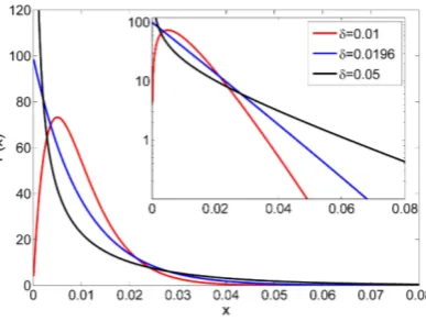
FIG. 2: The species abundance distributionPeq(x), given by Eq. (7) forS= 100 species, is plotted here vs. xfor three values

of δ. In all cases the SAD approximates a Gamma distribution, with shape factor α >1 forδ < δc = 0.0196 and α < 1 if

δ > δc≈0.0196. At the criticalδthe power vanishes and the distribution has almost pure exponential decay as demonstrated

in the semi logarithmic plot in the inset.

This is a very strong result, although it has not received its due attention in the literature. To compare directly the expression (6) to observed SADs we have extracted the single species probability distribution function by integrating outS−1 species to obtain, say,Peq(x1) (since all species are symmetric, we will denote it byPeq(x)). The result is,

Peq(x) =Ax

2

S(1δ−1)−1₍₁−_x)

2(S−1)

S (1δ−1)−1_{, (7)}

whereAis a normalization factor.

Eq. (7) is an exact formula that reduces to (4) whereS= 2, but in this section we are interested in its implication forS 1. In this parameter regimex1, since the typical fraction of a single species never substantially exceeds 1/S, as we shall see.

As mentioned, whenS1,Peq takes a Gamma distribution (power law followed by an exponential cutoff) form,

Peq ≈Axα−1e−βx, (8)

where the rate factorβ appears as thex1 limit of,

(1−x)2(SS−1)(

1

δ−1)−1≈e−βx, (9)

withβ= (2/δ)−3. The shape factorα=_S2(1_δ −1) will be greater than one (meaning that the distribution vanishes at zero and has a peak in the vicinity of 1/S) if

δ < δc= 2

S+ 2, (10)

while for δ > δc the distribution diverges at zero but is still integrable. These behaviors are illustrated in Figure 2. Whenα is small the distribution approaches the Fisher log series, and in general it corresponds to the generalized Fisher log series distribution that was discussed in [22]. Note that if δ > 2/3 the assumption x1 does not hold anymore; we will not consider this case here.

For a fully surveyed empirical community the species richnessS is given, so the only parameter in (7) which is left to be fitted is δ. This makes the fit less impressive, of course, but the model is more parsimonious and its results may be preferred, e.g., when applying Akaike information criterion that includes a penalty to discourage overfitting, in comparison with two parameter theories.

FIG. 3: Explaining the BCI plot species abundance distribution. The species abundance distribution of the BCI (1995 census) tropical forest is presented [light blue bars in the Preston plot (a), light blue circles in the double logarithmic (Pueyo) plot (b)], together with the best fit to the SAD predicted for a lottery game withδ= 0.0265 (Eq. 7) and the ZSM theory (parameters taken from [11],θ = 47.22,m= 0.1). Although the ZSM appears to give a better fit, it is clear that Chesson-Warner lottery game does provide the kind of hollow curve SADs that appear in empirical studies. Moreover, for the ZSM two parameters were used, whereas only one parameter was employed for the lottery game.

where the only fitted parameter isδ. Indeed the best fit was obtained forδ= 0.027, as expected. One can see that this one parameter fit is worse than the two-parameter fit using zero-sum multinomials (ZSM) statistics, but it is not unacceptable. Interestingly, when plotted using the double-logarithmic (Pueyo) plot instead of Preston plot the single parameter fit using (7) looks much better.

However, the value 1/40 (of a generation) for δ appears to be unrealistic. As mentioned in [21] the value of δ has been found to be around 1/5, and the order of magnitude in difference is too large to be neglected. Similarly, estimations of the corresponding numbers for trees in the whole Amazon basin [5] suggest that the most abundant species constitutes about 1% of the population (meaning that the “knee” appears for even smaller relative abundances) and the corresponding value ofδ, smaller than 1/200, again seems unrealistic.

Altogether, it appears that a storage model may provide the type of hollow-curve SADs that characterize empirical systems. Its flexibility is limited sinceαandβ are both determined byδ, and other theories provide better fits, still one may believe that adding another parameter (in a theory that takes into account spatial effects, for example) may solve this difficulty. The need to extend the lottery model and to include demographic noise isnot the inability of (7) to support fat-tailed SADs, but the following three arguments:

1. Conceptually, as mentioned above, we would like to find an SAD that depends onσE, not only onδ.

2. The empirical SAD (and the theoretical expression (7) with theδvalues that yield a decent fit) has support on small absolute numbers, meaning that extinction events must occur and are important, or, equivalently, that demographic noise must be taken into account.

3. The correlation time of the environmental variations needed to account for empirical datasets appears to be unrealistically short.

In any case, once extinctions are incorporated into the model one should include speciation events to balance the species richness; the resulting model is the TNTB which is discussed in the next section.

V. THE TNTB: STORAGE EFFECT, DEMOGRAPHIC NOISE AND SPECIATION

The time-averaged neutral theory of biodiversity deals with a community of species, all having the same average

xJ

101 102 103

Peq

(

x

)

10-4 10-3 10-2 10-1

<2

D=<2E

FIG. 4: The light blue circles represent the SAD obtained from a simulation of the TNTB model (see Appendix B), with σ2D = 2, σ2E = 0.25, δ= 10−4, ν = 10−3 and J = 104. The results represent an average over time, abundances have been

recorded every 106 _{elementary timesteps. The red straight line has a slope−1, and it fits the data perfectly up toσ}2

D/σE2, the

region dominated by demographic stochasticity. Gamma distribution, withα= 2 andβ= 0.01 is shown by the purple curve. The parametersαandβwere obtained from the fit to the data, and differ from the predictions of the storage theory, since the demographic noise and mutations significantly weaken the storage effect.

to δand σE, the correlation time and the amplitude of environmental variations, here one should take into account the per-birth chance of speciationν, and the strength of the demographic noise,σD. One should introduce these two processes together: without extinction, speciation will cause the number of species to grow unboundedly. Without speciation, demographic noise will lead to fixation by a single species in the long run.

The standard way to introduce speciation is to assume that an offspring carries the taxonomic identity of its mother with probability 1−ν, and is the originator of a new species with probabilityν (see details of our simulation technique in Appendix B). The strength of demographic stochasticity is defined as the variance in the number of offspring per individual σ2

D and usually takes a value between 2 (for a geometric distribution of offspring) and 1 (for a Poisson distribution). In the limit σE = 0, without environmental noise and storage effect, one obtains the metacommunity version of Hubbell’s neutral theory (or Kimura’s neutral model), where Peq (for a high-diversity system with 1/J < x1 ) is given by Fisher log-series,

PσE=0

eq (x) = A xe

−νJ x/σ2

D_{, (11)}

whereAis a normalization constant. The species richnessS reflects the balance between extinction and speciation

SσE=0₌₋ ν

σ2 D

log

ν σ2 D

J. (12)

What happens in TNTB, when the storage mechanism acts together with demographic noise and speciation events? Here we would like to emphasize a few generic features of this system:

1. Demographic stochasticity allows for extinction while speciation increases species richness, and the balance between these two processes is determined byδandσE. The lower the value ofδ, the sharper the SAD peak in the vicinity of 1/S, the time to extinction of a single species increases, and the chance of a low-abundance species to invade grows. Accordingly, the steady state species richnessS decreases monotonically with increasingδ.

Dynamically, when the chance of extinction is low the process of speciation acts to increase the number of species S,δc decreases (see Eq. 10) and the probability mass ofPeq in the regionx1 grows, leading to an increased rate of extinction until it balances the effect of speciation and the system reaches a steady state at finite S.

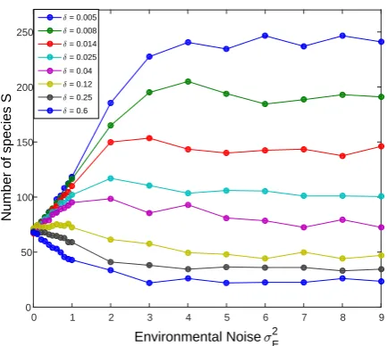
Environmental Noise <_E2

0 1 2 3 4 5 6 7 8 9

Number of species S

0 50 100 150 200 250

/ = 0.005

/ = 0.008

/ = 0.014

/ = 0.025

/ = 0.04

/ = 0.12

/ = 0.25

/ = 0.6

FIG. 5: S, the species richness, is plotted against σE2, the amplitude of the environmental stochasticity. The results were

obtained in simulations of a TNTB community withJ = 10000 and ν = 0.001 for various environmental correlation times δ (given in the legend in units of one generation). S reflects the balance between extinction and speciation; the lower is δ, the stronger is the storage effect and thusS increases. An increase in the strength of environmental variationσ2E may either

decreaseS (since it increases abundance variation) or increase the species richness by facilitating the storage effect. Here we see that the general trend depends on the value of δ. All the lines converge to the NTB limit,S =−J νlog(ν)∼= 70, when σE→0.

the TNTB has two regimes. For largexone observes (8), the storage power-lawα−1 followed by an exponential cutoff. Forx < σ_D2/σ2_Ethe powerα−1 is replaced by a 1/xdependence, a characteristic of the Fisher log-series.

Therefore, the conceptual problem raised in Section III, namely the fact that the theory of the storage effect predictsPeq to be independent of σE, is solved within the TNTB framework: the ratio σD2/σE2 determines the crossover from the 1/x decay to the behavior described by (8), and the SAD (and the overall species richness S) does depend on σE. In theσE→0 limit the TNTB converges to the standard neutral theory of Hubbell.

3. Given that, one may wonder about the effect of environmental stochasticity on species richness. On the one hand, σE is responsible for the storage effect that provides stability and allows for low abundance species to invade. On the other hand, (see Eq. (14) below and the following discussion) in systems without a storage effect [22, 28], environmental stochasticity clearly acts to lower S, as it increases the rate of extinction events since environmental fluctuations cause a species to visit more frequently the dangerous zone of low abundance.

Figure 5 solves this puzzle: it shows that the effect of environmental stochasticity on species richness, when all other parameters are kept fixed, is determined by the correlation time δ. For smallδ’s the storage effect wins and in general the species richness increases with the amplitude of environmental variations. For large values ofδ the increase in the system’s variability leads to a decrease inS.

4. The NTB was criticized by many authors for its strict commitment to perfect neutrality [36]. Under the rules of the neutral game, even the slightest fitness difference leads to a fixation of the system by the fittest species (in the absence of speciation) or to the appearance of an SAD that reflect Darwinian dominance, with one common species that occupies most of the community and a few rare, short lived, species [22]. The stabilizing effect of the storage mechanism resolves this difficulty. Even if the average fitness of different species is not the same, the system may still support high diversity.

To demonstrate this we have simulated the non-neutral modification of the TNTB, when the expression for fitness, Eq. (2), is replaced by

fi=eηi+γ

t

i_{, (13)}

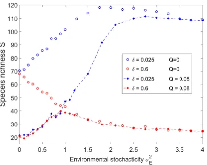
FIG. 6: S, the species richness, is plotted againstσ2

E, amplitude of the environmental stochasticity for simulations withQ= 0

(same as in Fig 5, empty circles) and for the case with time independent fitness differences (ηis) withQ= 0.08 (filled circles

connected by dashed lines). All other parameters are the same used in Figure 5. When σ2E = 0 time independent fitness

differences lead to a biodiversity collapse, where the fittest species is dominant and all other species are rare. On the other hand, whenσ2

E is large environmental noise washes out the effect of time independent fitness differences andS(Q) approaches

S(Q= 0). The species richness peaks at intermediate level of disturbance forδ= 0.6.

to a biodiversity collapse, as seen in Figure 6. However, as σE increases, the number of species grows since the storage effect induces stability. Finally at large σE the effect of fitness differences disappears and the species richness takes its Q= 0 value, as in the TNTB.

An interesting feature of the finite Qdynamics is the unimodal dependence of S on σ2

E when δ is sufficiently large. While weak environmental stochasticity stabilizes the species, strong variations lead to faster extinction and reduce S and biodiversity reaches a maximum under intermediate disturbance. One may expect such an effect in nonadditive systems (see [37]), and we believe that our model provides an appropriate framework for its analysis.

Before concluding this section, we would like to stress that environmental stochasticity and the storage effect are not synonymous. When the environmental variations affect only the death rate, or whenδ = 1, there is no storage effect andσE is a purely destabilizing factor. Even a slight modification of the rules governing the process may kill the storage effect. For example, in the lottery gameall the trees in the forest are competing for an open gap, where the chance of a species to win depends on its fitness. The pairwise competition version of the same game, where two individuals are picked at random and an offspring of one replaces the other with probability that depends on their relative fitness, has no significant storage effect. With respect to this specific duel all other trees play no role, so it corresponds to theδ= 1 case of the lottery game. Conversely, in the NTB limit (without environmental stochasticity) there is no difference between these two versions of the neutral game, see e.g. [11].

The SAD for TNTB without the storage effect (e.g., for the pairwise competition case) for 1/J < x 1 was calculated in [22],

P_eqno storage(x) =C x

1 + 2σ

2 EJ σ2

D x

−1−ν/σE2

(14)

where C is a normalization constant. Here the power law decay 1/x that characterizes the region dominated by demographic noise is replaced, forx > σ2

D/σ 2

E, by a power law with a larger exponent 2 +ν/σ 2 E.

VI. SUMMARY AND DISCUSSION

support a stable equilibrium the extinction time is exponential in the species’ abundance, while under unstable equilibrium, like in the neutral model, the time to extinction scales linearly with the abundance. To maintain the diversity of a metacommunity these timescales should be comparable with the evolutionary timescale that determines the rate at which new species enter the system and balance the diversity losses due to extinction.

A system that acquires its stability due to the storage effect is somewhere in-between. The stabilization is based on environmental stochasticity, which is, at the same time, a destabilizing force. As we have seen, the outcome of the competition between these two aspects of the same phenomenon - environmental stochasticity - is determined by one parameter, δ, the correlation time of the environment. If δ is large the destabilizing effects dominate and environmental stochasticity reduces biodiversity. When δ is small, as seen in fig 5, the stabilizing effect associated with the storage mechanism leads to an increase of extinction times and the overall biodiversity.

In the metacommunity version of Hubbell’s neutral theory, speciation and demographic drift are the only factors that govern the dynamics of the community, leading to the Fisher log-series SAD and species richness which is given by (12). The 1/xdecrease of the SAD at smallxdoes not fit the observed statistics on, say, the Barro Colorado Island and other local communities, where the slope is clearly weaker than 1/x (in a Preston plot, where the number of species in any abundance octave is plotted without normalization by the width of the octave, 1/xis translated into a straight horizontal line, while the Preston plots of empirical local communities show a unimodal behavior, see Fig 3a). To account for that, in the mainland-island version of NTB the statistics of a local community are governed by two parameters, the fundamental biodiversity number of the metacommunityθ= 2νJM/σ2D and the chance of migration to the island. The emerging zero-sum multinomial SAD fits the empirical evidence, as may be seen in Figure 3 above. Nevertheless the dynamics, in particular the rate of abundance variations, is too fast to be explained by the neutral model [16, 17, 21].

TNTB, that was shown to explain both static and dynamic patterns [21], has three extreme limits. WhenσE →0 it converges to the NTB, as environmental variations vanishes. WhenσD/σE→0 it converges to the classical lottery model of Chesson and Warner. The other limit isδ→1, when environmental noise does affect the system but there is no storage. The SADs in these three limits were presented in this paper (Eqs. 7, 11, 14).

In between, as showed in section IV, the situation is more complicated, and the way environmental stochasticity affects species richness is determined by the correlation timeδ. For short correlation times,Sis an increasing function ofσE, while for longer correlation times the situation is closer to the one discussed in [22] - a species may enjoy a long time in which its population grows, so the SAD widens and the overall species richnessSdecreases when environmental variations increase in amplitude.

AcknowledgmentsWe acknowledge the support of the Israel Science Foundation, grant no. 1427/15.

APPENDIX A: DERIVATION OF THE FOKKER-PLANCK EQUATION (3)

Our starting point is the recursion relation, Eq. (1).

xt+1₁ =xt₁(1−δ) +δ f1x t 1 f2xt2+f1xt1

(A1)

To translate this equation to the Fokker-Planck language, one would like to find the average change inx1betweent andt+ 1, ∆x1, and also its varianceV ar(x1) = (∆x1)2−(∆x1)2. The Fokker-Planck equation than takes the general form,

∂P(x1, t)

∂t =−

∂ ∂x1

∆x1P(x1, t)

+1 2

∂2 ∂x2

1

(V ar(x1)P(x1, t)) (A2)

The transition between (A1) and(A2) is justified if both the mean change and its variance are small (in comparison with x1) during a single timestep, such that a differential equation is an appropriate description of the process, see below.

To calculate ∆x1, Eq. (A1) should be written as (we have replacedx2by 1−x1, so from now on we regardx1asx.

∆x=xt+1−xt=xtδ

₁

(f2/f1)(1−xt) +xt −1

(A3)

Writingfi=eγi, and expanding ∆xin powers of ∆γ≡γ1−γ2, we have

∆x=xδ

∆γ(1−x) +1

2(1−x)(1−2x)(∆γ)

2_+O((∆γ)3 )

where the negligence of higher orders in ∆γ is justified if this quantity is small compared to one. Since ∆γ= 0 the first term in the r.h.s. of (A4) vanishes. The strength of the environmental stochasticity is defined viaσ2

E≡(∆γ)2, so we left with,

∆x≈ δσ 2 E

2 x(1−x)(1−2x). (A5)

Writing (∆x)2as the square of the r.h.s. of (A3), expanding to second order in ∆γ, averaging over ∆γand collecting the nonvanishing quantities one obtains,

∆x2≈σ2_Eδ2x2₁(1−x1)2 (A6)

Finally, keeping only second order terms in ∆γ,V ar(∆x)≈∆x2, and by plugging the results of (A5) and (A6) into (A2) one obtains Eq. (3) of the main text.

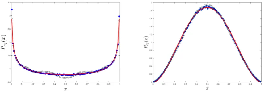
The replacement ofP(xt+1)−P(xt) by the time derivative ofP is allowed if the changes inxduring one timestep are small, i.e., ifδσ2

E 1. However, when comparing the results obtained from direct simulations of the recursion relation (1) and the predictions of the Fokker-Planck equation, say, (4), one finds that this approximation holds in a much wider regime, see Figs A1.

FIG. A1: The predictions of the Fokker-Planck equation (4) for Peq(x) (full line), are compared with Peq obtained from

numerical simulations of the recursion relation (1) for different values ofδ andδσ2

E. Forδ = 0.6 (left), the simulatedPeq at

σ2E= 1 (filled blue circles) is almost indistinguishable from the Fokker-Planck predictions, while forσ

2

E = 6 (open black circles)

one observes a few little humps. Forδ= 0.25 (right panel) the situation is even better, atσ2E= 1 the approximation is exact

and only forσ2

E= 100 (open black circles) slight deviations may be identified. For smaller values ofδwe were unable to identify

any deviations even for larger values, up toσ2

E= 10000.

Note that, as long as the transition to the Fokker-Plank equation (replacement of the recursion relation by a continuous in time differential equation) may be justified, the limit σE → ∞ is quite trivial. In this limit with probability 1/2 xt+1=xt(1−δ) and with probability 1/2xt+1=xt+δ(1−xt). Accordingly, ∆x=δ(1−2x)/2 and V ar(x) =δ2/4. The resulting Fokker-Planck equation has anx-independent diffusion term: it does not vanish on the edges, since growth is independent of the abundance. This leads to

Peq(x)∼e

4x(1−x)

δ _{, (A7)}

meaning that the distribution in this limit is a Gaussian aroundx= 1/2. In fact, writingy=x−1/2 and expanding for smallyboth (4) and (A7) converge toexp(−4y2/δ), and for smallδ(where the deviations fromx= 1/2 are small) higher orders inyare negligibly small. Therefore (see Fig. A1 and its caption) as long asδis small it is quite difficult to find any difference between the prediction of (4) and the results of simulations at largeσ2

E. A similar argument for S species yieldsPeq(x)∼exp(−(x−1/S)2/w wherew=S/(δ[1−1/S]).

APPENDIX B: SIMULATING THE DYNAMICS OF A COMMUNITY

We start withJ individuals, each belongs to one ofS species, and each species ihas a fitnessfi=exp(γi), where the values ofγi are picked from a normal distribution with zero mean and widthσE.

During an elementary timestep one individual is chosen (at random, independent of its species affiliation) to die. If the dying individual is a singleton, the number of species is reduced by one. Then, with probabilityν, this individual is replaced by the originator of a new species, the number of species in the system grows by one and a fitness is assigned to the new species using the procedure described above.

With probability 1−ν the individual is replaced by a descendent of another individual that inherits its parent identity. The chance of the speciesito capture the empty slot is given byfixi/P

S

j=1fjxj, wherexi is the abundance of speciesi(an integer). after each elementary timestep the time grows by 1/J.

When the time reaches δ (after δJ elementary steps) all the fitness values fi are picked for all species using the same procedure, with no correlation between the new and the old fitness. This implies that the correlation time of the environmental variations isδof a generation.

[1] G. F. Gause,The struggle for existence(Courier Corporation, 2003). [2] G. Hardinet al., Science131, 1292 (1960).

[3] G. E. Hutchinson, American Naturalist , 137 (1961).

[4] M. Stomp, J. Huisman, G. G. Mittelbach, E. Litchman, and C. A. Klausmeier, Ecology92, 2096 (2011).

[5] H. Ter Steege, N. C. Pitman, D. Sabatier, C. Baraloto, R. P. Salom˜ao, J. E. Guevara, O. L. Phillips, C. V. Castilho, W. E. Magnusson, J.-F. Molino,et al., Science342, 1243092 (2013).

[6] S. R. Connolly, M. A. MacNeil, M. J. Caley, N. Knowlton, E. Cripps, M. Hisano, L. M. Thibaut, B. D. Bhattacharya, L. Benedetti-Cecchi, R. E. Brainard,et al., Proceedings of the National Academy of Sciences111, 8524 (2014).

[7] P. Chesson, Annual review of Ecology and Systematics31, 343 (2000). [8] D. Gravel, F. Guichard, and M. E. Hochberg, Ecology letters14, 828 (2011). [9] P. Amarasekare, Ecology Letters6, 1109 (2003).

[10] S. P. Hubbell,The unified neutral theory of biodiversity and biogeography (Princeton University Press, 2001). [11] I. Volkov, J. R. Banavar, S. P. Hubbell, and A. Maritan, Nature424, 1035 (2003).

[12] J. Rosindell, S. P. Hubbell, and R. S. Etienne, Trends in Ecology & Evolution26, 340 (2011). [13] R. E. Ricklefs, Ecology87, 1424 (2006).

[14] S. Nee, Functional Ecology19, 173 (2005).

[15] E. G. Leigh, Journal of Evolutionary Biology20, 2075 (2007).

[16] M. Kalyuzhny, Y. Schreiber, R. Chocron, C. H. Flather, R. Kadmon, D. A. Kessler, and N. M. Shnerb, Ecology95, 1701 (2014).

[17] M. Kalyuzhny, E. Seri, R. Chocron, C. H. Flather, R. Kadmon, and N. M. Shnerb, The American Naturalist184, 439 (2014).

[18] R. A. Chisholm, R. Condit, K. A. Rahman, P. J. Baker, S. Bunyavejchewin, Y.-Y. Chen, G. Chuyong, H. Dattaraja, S. Davies, C. E. Ewango,et al., Ecology Letters17, 855 (2014).

[19] R. A. Chisholm and J. P. ODwyer, Theoretical population biology93, 85 (2014). [20] M. Danino and N. M. Shnerb, Physical Review E92, 042706 (2015).

[21] M. Kalyuzhny, R. Kadmon, and N. M. Shnerb, Ecology letters18, 572 (2015). [22] D. A. Kessler and N. M. Shnerb, Journal of Theoretical Biology345, 1 (2014).

[23] S. Azaele, S. Suweis, J. Grilli, I. Volkov, J. Banavar, and A. Maritan, Reviews of Modern Physics (2016). [24] P. L. Chesson and R. R. Warner, American Naturalist , 923 (1981).

[25] P. Chesson, Theoretical Population Biology45, 227 (1994).

[26] J. S. Hatfield and P. L. Chesson, Theoretical Population Biology36, 251 (1989).

[27] J. Ohkubo, N. Shnerb, and D. A. Kessler, Journal of the Physical Society of Japan77, 044002 (2008). [28] D. Kessler, S. Suweis, M. Formentin, and N. M. Shnerb, Phys. Rev. E92, 022722 (2015).

[29] R. Lande, S. Engen, and B.-E. Saether,Stochastic population dynamics in ecology and conservation (Oxford University Press, 2003).

[30] S. P. Hubbell,The unified neutral theory of biodiversity and biogeography, Monographs in Population Biology 32 (Princeton University Press, Princeton, N.J., 2001).

[31] W. Ulrich, M. Ollik, and K. I. Ugland, Oikos119, 1149 (2010).

[32] S. Azaele, S. Pigolotti, J. R. Banavar, and A. Maritan, Nature444, 926 (2006).

[33] S. Azaele, A. Maritan, S. J. Cornell, S. Suweis, J. R. Banavar, D. Gabriel, and W. E. Kunin, Methods in Ecology and Evolution6, 324 (2015).

[34] J. S. Hatfield and P. L. Chesson, inStructured-Population Models in Marine, Terrestrial, and Freshwater Systems(Springer, 1997) pp. 615–622.

[35] J. H. Gillespie, Theoretical Population Biology17, 129 (1980). [36] S.-R. Zhou and D.-Y. Zhang, Ecology89, 248 (2008).