Estimation of New Monetary Valuations of Travel Time, Quality of Travel, and Safety for Singapore

79 Transportation Research Record: Journal of the Transportation Research Board, No. 2664, 2017, pp. 79–90.

http://dx.doi.org/10.3141/2664-09

A large-scale study in Singapore estimated new monetary valuations for travel time, quality of travel, and safety covering different modes and journey components. A wide-ranging stated-choice survey was con-ducted on a large, representative sample. The empirical work pushed the boundaries of the international state of the practice in choice model-ing by relymodel-ing on mixed logit models with all model components bemodel-ing random and a full covariance matrix being estimated. Detailed results are presented, and the values are contrasted with those from the previous study, conducted in 2008.

The Land Transport Authority (LTA) is the government agency tasked with the development and regulation of Singapore’s land transport sys-tem. In common with many other such agencies around the world, LTA uses cost–benefit analysis as part of its overall appraisal framework in determining the merits of new transport policies and infrastructure developments. For this analysis, social benefits such as travel time savings, reliability improvements, crowding reduction, and accident cost savings need to be quantified. Willingness-to-pay (WTP) measures are critical inputs into this process, and in common with many other nations, LTA uses values produced through the estimation of discrete choice models on stated-preference data (1–4).

With the major societal, economic, and environmental implications of new policy and infrastructure schemes, it is important that these WTP measures have a high level of reliability. This requirement means that the values should be updated at regular intervals given not only the changing nature of transport systems and travel behavior but also ongoing improvements to survey and modeling approaches.

Because the most recent WTP estimates date from 2008, LTA com-missioned a new study in 2015, with a large-scale data collection effort and the estimation of advanced choice models; these models offered improvements in flexibility over those used in 2008. What sets the resulting study apart is the relative size of the sample compared with the population of Singapore, the breadth of modes and journey components covered, and the use of a highly flexible treatment of heterogeneity. This last point ensures a methodological contribution in addition to the development of new results for policy work.

Survey Work

Sampling

A total of 5,000 households were selected for interview between May and November 2015, representing a very large sample from a population of around 5.6 million people. Quotas were developed by travel mode, journey purpose, period of travel, age, and gender; this method ensured sufficiently large sample sizes for the modeling work for each mode as well as representative samples for other dimensions. The study sampled car, motorcycle, mass rapid transit (MRT), bus, and taxi users as well as pedestrians and cyclists.

The vast majority of interviews were carried out in respondents’ homes using tablets. These data were supplemented with some observations from an island-wide intercept survey. On successful completion of a survey, each respondent was given a $10 online shopping voucher as a reward.

Before the analysis, the sample was compared with the 2012 household travel survey (HTS) data to test its representativeness. Although this comparison showed small discrepancies, such as a slightly higher percentage of 35- to 54-year-olds and female respon-dents in the survey, the overall match was also very good in terms of dwelling types, vehicle ownership, ethnic breakdown, employment status, and income distribution.

Survey Content and Design

Stated preference, and in particular stated choice (SC), is a widely used technique for value-of-time (VTT) research (2). Respondents are faced with a number of carefully designed hypothetical choice scenarios, in which two or more alternatives are described by key attributes such as travel time and travel cost, and respondents are asked to select their preferred option in each.

There is ongoing debate in the academic literature about the rela-tive merits of simple and complex surveys. Much of the northern European evidence is based on the most simplistic surveys with two alternatives and two attributes [compare with the discussion by Hess et al. (2)]. However, the work in Australia especially tends to rely on at least three alternatives in each choice task, with often five or six attributes describing them (5). In the current work, a balance was struck between these two extremes. Although a binary context was retained, a larger number of attributes was used to describe these alternatives. With substantial differences across the various measures of interest (e.g., VTT versus value of safety), the choice tasks for each respondent were spread across different survey contexts, or games; this method also helped to reduce the respondent burden.

Estimation of New Monetary Valuations

of Travel Time, Quality of Travel,

and Safety for Singapore

Stephane Hess, Paul Murphy, Henry Le, and Wai Yan Leong

80 Transportation Research Record 2664

An overview of the different SC games is given in Table 1, where, for example, car users faced 15 choice tasks spread across three dif-ferent games. For the majority of attributes, the researchers sought to increase the realism by pivoting the values presented to respon-dents around the attributes from a recent trip for that respondent. The actual designs were produced by using NGene (http://www .choice-metrics.com) with Bayesian D-efficiency as a criterion for the statistical properties of the designs (6), priors coming from the 2008 study (7), and avoidance of the inclusion of strictly dominant alternatives by using a regret measure (8). The majority of the games are of such standard nature that no details are required beyond those in Table 1. However, special attention is needed for accident games (CA1, MCA1, PA1, and CYA1), crowding games (MT1 and BT1), and the game for bus excess waiting time (BT2).

The purpose of the accident games is to derive a WTP measure for reducing the number of different types of accidents and hence also the WTP measure for reducing personal risk. A standard approach [e.g., that by Hensher et al. (9)] involves presenting respondents with a choice between two routes described in terms of travel time, the number of accidents by injury types, and some monetary cost, with the choice framed around a recent journey and accident rates presented, for example, as: “Number of deaths per year along the route.” In the work by Hensher et al., this number goes from 0 to 5, which is of course very high for a single road (9).

In the case of Singapore, where the total number of accidents is far lower, presenting by road and route rates is even more unrealistic. There is also an issue with exposure because only part of someone’s annual travel will be on this route, and a disconnect between the payment mechanism (per trip) and the accident numbers (per year). A per-journey cost also makes the method inapplicable for pedes-trians and cyclists. Instead a programmed approach is relied on, in which the choice is between two national safety programs and the payment mechanism is a change in the annual tax burden. The two programs are described in terms of increases or decreases in tax

(per year), along with annual figures for fatalities and serious and minor injuries.

MT1 and BT1 consider the sensitivity to in-vehicle travel time in different conditions: waiting time, walking time, and interchanges. Rather than a simple presentation of overall numbers for a journey and a single level of crowding, journeys are broken up into differ-ently sized stages (Figure 1). The presentation allows for changes in crowding that are the result of either changing to a different bus or train or other passengers’ joining or leaving the bus or train on which the respondent is already traveling.

BT2 is concerned with bus reliability. LTA uses the concept of excess wait time (EWT), in which, on the assumption of a uniform arrival rate of passengers, EWT is the average additional wait time actually experienced compared with the expected wait time if buses arrived at regular intervals. It is defined as the difference between actual wait time (AWT) and the scheduled wait time (SWT); that is, EWT = AWT − SWT:

n n

n n

∑

∑

= ×

AWT

actual headway

2 actual headway

2

n n

n n

∑

∑

= ×

SWT

scheduled headway

2 scheduled headway (1)

2

EWT increases if there is bus bunching, which results in prolonged waits for the subsequent bus. Respondents had a choice between two future hypothetical bus services (Figure 2), for which the scheduled arrival time of the bus is shown every 10 min, along with the interval between buses for both options and the bus fare. It is assumed that buses arrive frequently enough that users forget the timetable; in other words, their arrival time at the bus stop is completely arbitrary.

TABLE 1 Summary of SC Games

Game Description Attributes

Choice Tasks

CT1 Car: congestion and costs Free-flow travel time, light congestion, heavy congestion, parking cost, petrol cost, ERP cost 5 CT2 Car: parking choice Walking time, queuing time, search time, parking cost 5 CA1 Car: accidents Fatalities, serious and minor injuries per year, change in annual tax burden 5 MCT1 Motorcycle: congestion and costs Free-flow travel time, light congestion, heavy congestion, parking cost, petrol cost, ERP cost 7 MCA1 Motorcycle: accidents Fatalities, serious and minor injuries per year, change in annual tax burden 5 MT1 MRT: time and crowding Walking time, waiting time, in-vehicle time in five crowding levels (3 seated, 2 standing),

interchanges, fare 7

MT2 MRT: walking Crossing type (at grade, uncovered bridge, covered bridge without lift, covered bridge with lift, air-conditioned underpass, covered and uncovered walking time to and from crossing, fare

7

BT1 Bus: time and crowding Walking time, waiting time, in-vehicle time in five crowding levels (3 seated, 2 standing), interchanges, fare

7

BT2 Bus: excess waiting time Bus arrival times, fare 7 TT1 Taxi: access, time, and costs Walking time, waiting time, in-vehicle time, prebooked or on street, fare, booking fee 7 PT1 Pedestrian: walking environment Crossing type (at grade, uncovered bridge, covered bridge without lift, covered bridge with

lift, air-conditioned underpass, covered and uncovered walking time to and from crossing 7 PA1 Pedestrian: accidents Fatalities, serious and minor injuries per year, change in annual tax burden 5 CYA1 Cycling: accidents Fatalities, serious and minor injuries per year, change in annual tax burden 5

MoDeling FraMeWork

In the past four decades, choice models have undergone major devel-opments in terms of flexibility, especially in terms of the presentation of heterogeneity in preferences across individual decision makers (10). As a result, there have been substantial improvements to the techniques used in VTT studies, most notably starting with the work in Denmark (4) and more recently in the context of the British VTT study (2). In what follows, the focus is only on what is relevant for the current study, largely because of space considerations.

In a random utility model, the utility Uint that individual n (out of N) obtains from choosing alternative i (out of I) in choice situation t (out of Tn) is decomposed into an observed component Vint and a random component εint. Almost all applications rely on an additive error structure, with Uint= Vint+εint, in which noise is independent of observed utility. Recent work by Fosgerau and Bierlaire has ques-tioned this specification and put forward a multiplicative formulation, in which errors are proportional to observed utility, with Uint= Vint•ε_int (11). In practice, this formula implies more noise on longer trips, a notion that has received empirical support in the Danish (4) and

British (2) national studies. The two specifications in early work were compared and no evidence was found of an improvement with the multiplicative structure, so the additive structure was retained. Part of the reason for the lack of improvement could be the smaller size of Singapore and the resulting much-reduced heterogeneity in trip distances.

Next, the specification of the observed component of utility is con-sidered. Using the example of CT1, the following formula would be written:

FF LC HC ERP

petrol parking (2)

FF LC HC ERP

petrol parking

= β + β + β + β + β + β

Vint int int int int

int int

where

FF = free-flow time,

LC = time spent in light congestion, HC = time spent in heavy congestion, and ERP = electronic road pricing.

(a)

(b)

82 Transportation Research Record 2664

ERP, petrol, and parking costs are cost attributes, and six β-terms would be estimated giving the marginal utilities for the associated attributes.

The VTT in free-flow conditions expressed in terms of ERP cost sensitivity would then, for example, be given by

VTTFF,ERP FF ERP

= β β

This expression indicates how much increase in ERP would be acceptable in return for a 1-min reduction in free-flow time. Although these computations are straightforward in models with fixed β, this is no longer the case when random heterogeneity is allowed for (12). To avoid the need to divide by random coefficients, the mathematically equivalent approach working in WTP space is used instead (13), again with ERP as the base cost:

V VTT FF VTT LC

VTT HC ERP

petrol parking (3)

ERP

FF,ERP LC,ERP HC,ERP

petrol parking

= β +

+ +

 

  + β + β

int

int int

int int

int int

where VTTFF,ERP is now estimated directly.

Each respondent in the surveys was faced with choice tasks from multiple different games. Although joint estimation would be

advisable if valuations were consistent across games, preliminary work showed differences in valuations across games (not surprising given the differences in context), and the analysis was carried out on a game-specific level, except for merging MT2 and PT1 in the absence of a cost attribute for the latter.

Initial attempts to unearth links between key sociodemographic variables (e.g., income and age) and patterns in VTT were largely unsuccessful, and it was suspected that unexplained heterogeneity dominated. The work in this context relies on mixed multinomial logit models [see, e.g., Chapter 6 in the work by Train (10)], as is now common practice in many national VTT studies (1–4). Let Pint(β) give the probability that respondent n will choose alternative i in choice task t, conditional on a vector of parameters β, where with εint following a Type I extreme value distribution,

1 2

∑

( )

=

P e

e

int

V V j

int

jnt

The probability of the sequence of Tn choices for individual n is given by

∑

∏

( )

= =

1 2 1

*

P e

e

int

V V j t T i nt

jnt n

Bus BT2 waiting time

I would choose

where Vi*nt refers to the utility of the alternative n actually chosen

in task t.

It is assumed that the vector β follows a random distribution across respondents, with β~ f(β|Ω), with Ω a vector of estimated parameters. Then

(4)

∫

( )

(

)

( )Ω = β β Ω β

β

Pn Pn f d

Studies using mixed multinomial logit typically allow for heteroge-neity in only some elements of β and impose independence between those. As discussed by Hess and Rose (14), the first of these assump-tions will invariably lead to a lower fit and potential confounding in terms of the source of heterogeneity. The second assumption will also lead to a lower fit and may overstate the heterogeneity in relative sensitivities.

In this work, all parameters were instead allowed to vary randomly across respondents, with a full covariance matrix estimated between them. To the best of the authors’ knowledge, this is the first such appli-cation in the context of a national VTT study and is also far beyond the level of flexibility used in the majority of most small-scale academic applications.

With K elements in β, K mean sensitivities would be thus esti-mated as well as ∑k=1,...,K k elements in the covariance matrix of β.

This flexibility comes at the cost of increased model complexity, and classical estimation techniques were found to be unsuitable in terms of computational cost and their ability to find meaningful solutions. Instead Bayesian estimation was used, as discussed, for example, by Train (10, Chapter 13), specifically the implementation in Resource Systems Group Hierarchical Bayesian (RSGHB) (15).

As mentioned earlier, the initial exploration of the data failed to retrieve meaningful sociodemographic interactions, and the mixed multinomial logit models were specified without deterministic hetero-geneity on top of the random heterohetero-geneity. After model estimation, posterior estimates were produced (10, Chapter 11), which are then used in posterior segmentation work to attempt to uncover further deterministic heterogeneity. Let L(Yn|β) give the probability of observ-ing the sequence of choices Yn made by respondent n, conditional on a specific value of the vector β. The probability of observing a specific value of β is then given by the Bayes rule as follows:

(5)

∫

(

(

)

)

(

(

)

)

(

)

β β Ω β

β

L Y L Y f

L Y f d

n

n n

It is then possible to simulate, for example, the most likely value for β for respondent n as follows:

1 (6) 1

∑

∑

(

)

(

)

where βr with r = 1, . . . , R is an R independent multidimensional draw from f (β|Ω).

reSultS

Because of space considerations, a detailed account of the results for the CT1 and MCT1 games is given, with only overview results for the other games.

games for Car and Motorcycle in-vehicle time: Ct1 and MCt1

Negative lognormal distributions were used for the three cost com-ponents and the models in WTP space relative to ERP costs for the three time measures; positive lognormal distributions were used, with a full covariance matrix between the six terms. The three VTT measures were specified in an additive manner, such that a positive value of free-flow time, a positive increase in that value for travel in light congestion, and an increase on that value for travel in heavy congestion were estimated.

The means of the posterior distributions shown in Table 2 cor-respond to maximum likelihood estimates of the individual parameters (10, Chapter 13). These relate to the underlying normal distributions (a lognormal is given by an exponential of a normal), where the 15 elements of the covariance matrix use a numbering reflecting the order of presentation of the mean parameters. With Bayesian techniques, a standard error for individual parameters that would be suited for calculating t-ratios is not obtained but instead the posterior standard deviation is reported for each parameter. As expected, the relative variation in the posteriors is larger for MCT1 than CT1, given the lower sample size for the former.

As a next step, VTT measures were produced on the basis of Table 2. The lognormal has a very long tail, and a few outlying values can lead to extreme means (16). With this in mind, the distributions were censored by removing 1% of the highest values of the WTP distributions. Censoring is a controversial process but is required in some cases (17). However, it is crucial to ensure that it leads to a distribution that still represents the behavior in the data. Thus the censored distributions were used to recalculate the log likelihood of the model. For CT1, this calculation led to a minor drop in log likelihood to −3,473.41 (i.e., a drop of 0.73 unit), showing very little support in the data for extreme values. That is, the tail is driven by the overall shape of the distribution rather than the data. For MCT1, there was also only a small drop to −319.34 (by 1.19 units). More extreme censoring quickly led to substantial drops in fit; this result suggests that there is support in the data for the tail of the distribution up to the 99% point. The censoring led to much more realistic VTT measures; for example, the final weighted mean for CT1 travel time is 47 cents/min compared to 75 cents/min.

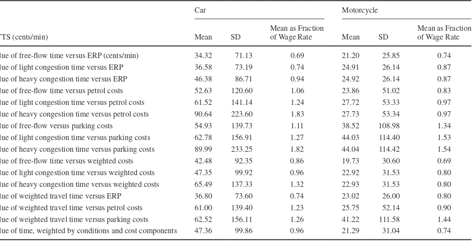
A wide range of valuations can be calculated from the estimates, as reported in Table 3. These values including the VTT against a weighted cost component, calculated at the level of each individual based on their split in cost components, and the VTT in average travel conditions, calculated for each individual based on their split in travel components observed in the data. With the individual components now all following imperfectly correlated random distributions, the individual mean values cannot be obtained simply as ratios of other means. In addition, the relative VTT in different travel conditions is not constant across the three cost components as a result of the heterogeneity in each component. Finally, with a random coefficients model, it is not appropriate to now calculate simple congestion multipliers.

TABLE 2 Estimation Results for CT1 and MCT1

CT1 MCT1

Attribute Posterior Mean Posterior SD Posterior Mean Posterior SD

VTT free flow versus ERP (underlying normal mean for log of coeff.) −2.33 0.20 −2.13 0.30 VTT light congestion shift versus ERP (underlying normal mean for log of coeff.) −6.33 0.67 −3.47 0.64 VTT heavy congestion shift versus ERP (underlying normal mean for log of coeff.) −4.18 0.38 −9.61 1.74 ERP (underlying normal mean for log of negative of coeff.) −0.51 0.13 0.11 0.18 Petrol costs (underlying normal mean for log of negative of coeff.) −0.97 0.14 0.39 0.19 Parking costs (underlying normal mean for log of negative of coeff.) −0.88 0.12 0.24 0.19

cov (1, 1) 3.30 0.84 1.37 0.93

cov (1, 2) 2.57 1.08 0.08 0.62

cov (1, 3) 2.49 1.60 −0.03 0.75

cov (1, 4) −1.19 0.62 −0.23 0.59

cov (1, 5) −0.79 0.48 −0.21 0.57

cov (1, 6) −0.95 0.53 −0.44 0.66

cov (2, 2) 7.33 2.54 0.43 0.43

cov (2, 3) 5.53 1.49 −0.04 0.44

cov (2, 4) −3.36 0.79 −0.11 0.38

cov (2, 5) −4.32 1.21 −0.01 0.33

cov (2, 6) −4.28 1.04 −0.08 0.40

cov (3, 3) 5.18 2.24 0.52 0.75

cov (3, 4) −2.83 0.86 0.04 0.40

cov (3, 5) −3.34 0.74 −0.02 0.29

cov (3, 6) −3.38 0.79 0.02 0.67

cov (4, 4) 1.87 0.48 0.70 0.38

cov (4, 5) 2.15 0.42 0.12 0.30

cov (4, 6) 2.11 0.40 0.10 0.34

cov (5, 5) 3.09 0.64 0.41 0.34

cov (5, 6) 2.94 0.48 −0.06 0.26

cov (6, 6) 3.03 0.51 0.68 0.49

Note: Cov = covariance. For CT1: respondents = 1,192; observations = 5,960; estimated parameters = 27; log likelihood =−3,472.68; adjusted r2= .15.

For MCT1: respondents = 107; observations = 749; estimated parameters = 27; log likelihood =−318.15; adjusted r2_{= .34.} TABLE 3 Implied In-Vehicle VTT Measures for Cars and Motorcycles: Means and SDs Across Sample

Car Motorcycle

VTTS (cents/min) Mean SD

Mean as Fraction

of Wage Rate Mean SD

Mean as Fraction of Wage Rate

Value of free-flow time versus ERP (cents/min) 34.32 71.13 0.69 21.20 25.85 0.74 Value of light congestion time versus ERP 36.58 73.19 0.74 24.91 26.14 0.87 Value of heavy congestion time versus ERP 46.38 86.71 0.94 24.92 26.14 0.87 Value of free-flow time versus petrol costs 52.63 120.60 1.06 23.86 51.02 0.83 Value of light congestion time versus petrol costs 61.52 141.14 1.24 27.72 53.33 0.97 Value of heavy congestion time versus petrol costs 90.64 223.60 1.83 27.73 53.34 0.97 Value of free-flow versus parking costs 54.93 139.73 1.11 38.52 108.98 1.34 Value of light congestion time versus parking costs 62.78 156.91 1.27 44.03 114.40 1.53 Value of heavy congestion time versus parking costs 89.99 233.25 1.82 44.04 114.42 1.54 Value of free-flow time versus weighted costs 42.48 92.35 0.86 19.73 30.60 0.69 Value of light congestion time versus weighted costs 47.35 99.92 0.96 22.92 31.53 0.80 Value of heavy congestion time versus weighted costs 65.49 137.33 1.32 22.93 31.53 0.80 Value of weighted travel time versus ERP 36.80 73.60 0.74 23.02 26.00 0.80 Value of weighted travel time versus petrol costs 61.00 139.40 1.23 25.75 52.14 0.90 Value of weighted travel time versus parking costs 62.52 156.11 1.26 41.22 111.58 1.44 Value of time, weighted by conditions and cost components 47.36 99.86 0.96 21.29 31.04 0.74

suggests that respondents did not react to these attributes in a mean-ingful manner. The finding is in line with some empirical evidence in other studies showing that respondents do not react realistically to petrol costs in journey-based choice experiments.

After model estimation, posterior distributions were produced and the conditional means were used for further analysis the focus of which is on the valuations against ERP. In Table 4, only those sociodemographics are reported for which a meaningful effect was observed. For car, there is clear evidence to suggest higher VTT measures for home-based-work travel and non-home-based travel, and an indication of higher VTT for those who obtain compensa-tion for their travel costs. For both modes, the values are highest for those who are employed and also higher for off-peak than for peak

travel, potentially suggesting some self-selection of higher VTT respondents into the off-peak periods. No clear patterns could be observed in terms of income or group size effects for either mode.

Summary results for other, nonaccident games

The results for the other, nonaccident games are discussed next (Table 5). Except where otherwise noted, positive lognormal distri-butions were relied on for WTP measures and negative lognormal distributions for cost. Except for the different approach in BT2, a 1% censoring was always applied to the lognormal tails. This procedure led to minor drops in fit for BT1 (3.5 units) and MT1 (0.43 unit) and

TABLE 4 Posterior Analysis for In-Vehicle VTT Measures for CT1 and MCT1

Variable Sample Size

Value of Free-Flow Time versus ERP (cents/min)

Value of Light Congestion Time versus ERP (cents/min)

Value of Heavy Congestion Time versus ERP (cents/min)

Value of Weighted Travel Time versus ERP (cents/min)

CT1

No purpose 4 27.86 30.65 43.02 30.91

HBO 352 34.34 36.46 45.72 36.68

HBS 171 29.88 31.70 39.74 31.92

HBW 327 37.29 39.84 50.68 40.04

NHB 338 37.01 39.48 49.98 39.68

Work FT, PT, or SE 737 36.88 39.35 49.92 39.55

Homemaker 139 31.15 32.97 41.02 33.20

Student 165 32.76 34.75 43.45 34.96

Retired 37 35.63 38.38 50.13 38.73

Unemployed or work not applicable 114 33.14 35.17 43.94 35.37

a.m. peak 454 34.66 36.92 46.62 37.12

p.m. peak 293 34.38 36.62 46.22 36.84

Combined peak 747 34.55 36.80 46.46 37.01

Off peak 445 36.40 38.78 49.04 38.99

Not compensated 1,141 34.93 37.22 47.07 37.43

Fully or partly compensated 51 42.30 44.78 55.41 44.95 MCT1

No purpose 0 na na na na

HBO 18 21.53 25.12 25.13 23.28

HBS 0 na na na na

HBW 57 23.25 26.96 26.96 25.07

NHB 32 19.50 23.29 23.30 21.36

Work FT, PT, or SE 96 22.92 26.65 26.66 24.75

Homemaker 3 12.22 15.60 15.61 13.87

Student 3 19.12 23.00 23.01 21.02

Retired 2 6.74 9.98 9.98 8.33

Unemployed or work not applicable 3 9.71 13.12 13.13 11.38

a.m. peak 45 20.53 24.25 24.26 22.36

p.m. peak 24 18.55 22.20 22.21 20.33

Combined peak 69 19.84 23.54 23.54 21.65

Off peak 38 25.47 29.21 29.22 27.31

Not compensated 96 22.14 25.84 25.85 23.95

Fully or partly compensated 11 19.26 23.03 23.04 21.11

Note: HBO = home-based other; HBS = home-based shopping; HBW = home-based work; NHB = non–home based; FT = full time; PT = part time; SE = self-employed;

86 Transportation Research Record 2664

small gains in fit for CT2 (0.15 unit), TT1 (0.53 unit), and MT2-PT1 (5.92 units). Overall, these results confirm little empirical support for the extreme values and justify the censoring approach.

Car Out-of-Vehicle Time Game (CT2)

Respondents are on average most sensitive to searching time ahead of walking time and queueing time, in which no constraints on the ordering were imposed. The actual valuations are lower than

those obtained in CT1; a possible reason is that out-of-vehicle times are on average much shorter (11.8 min) than in-vehicle times (27 min) in this sample. There is substantial empirical evidence elsewhere (2) to support the notion that VTT measures are higher on longer journeys.

Taxi Game (TT1)

For TT1, a normal distribution was used as the constant for booked taxi services, and no constraints on ordering were imposed.

Respon-TABLE 5 Summary Valuations for Nonaccident Games Other Than CT1 and MCT1

Variable Mean SD

Mean as Fraction of Wage Rate

CT2 (cents/min)

Value of walking time 36.39 142.66 0.74

Value of queueing time 32.62 132.12 0.66

Value of searching time 40.02 186.07 0.81

TT1 (cents/min)

Value of walking time 54.97 102.89 1.28

Value of in-vehicle time 55.27 85.34 1.28

Value of waiting time 61.59 133.90 1.43

BT1 (cents/min except where indicated)

Value of walking time 15.96 30.76 0.53

Value of waiting time 15.06 34.85 0.50

Value of interchanges (cents/interchange) 40.82 122.89 na Value of in-vehicle time, seated, with empty seats 10.67 25.34 0.35 Value of in-vehicle time, seated, quite packed 10.88 25.42 0.36 Value of in-vehicle time, seated, completely packed 13.01 25.60 0.43 Value of in-vehicle time, standing, quite packed 16.55 30.38 0.55 Value of in-vehicle time, standing, completely packed 17.01 30.66 0.56 Value of vehicle time weighted by crowding conditions 11.73 25.39 0.39 MT1 (cents/min except where indicated)

Value of walking time 22.83 46.67 0.67

Value of waiting time 17.00 32.91 0.50

Value of interchanges (cents/interchange) 68.16 287.24 na Value of in-vehicle time, seated, with empty seats 17.39 43.20 0.51 Value of in-vehicle time, seated, quite packed 17.78 43.39 0.52 Value of in-vehicle time, seated, completely packed 18.01 43.44 0.53 Value of in-vehicle time, standing, quite packed 22.08 48.39 0.65 Value of in-vehicle time, standing, completely packed 24.50 50.40 0.72 Value of vehicle time weighted by crowding conditions 20.71 46.21 0.61 BT2

Value of EWT (cents/min) 71.74 144.75 2.38

MT2 and PT1 Combined

Value of uncovered walking time (cents/min) 15.47 27.43 0.51 Value of covered walking time (cents/min) 5.71 10.93 0.19 Value of crossing time (cents/min) 10.79 22.73 0.36 WTP for avoiding covered bridge with lift versus air-conditioned underpass (cents/crossing) 13.56 16.74 na WTP for avoiding covered bridge without lift versus air-conditioned underpass (cents/crossing) 24.68 40.44 na WTP for avoiding uncovered bridge without lift versus air-conditioned underpass (cents/crossing) 52.11 45.27 na WTP for avoiding road crossing versus air-conditioned underpass (cents/crossing) 13.96 20.60 na

dents are on average most sensitive to waiting time, with no differ-ence between in-vehicle time and walking time in the mean, although the latter has a higher standard deviation. Walking time is on aver-age much shorter than in-vehicle time in this sample (1.8 min versus 22.6 min), and the findings could thus relate to a lower value of small time savings. The actual valuations are higher than the wage rate, but this finding needs to be placed in the context that taxi journeys are infrequent, and travelers are willing to pay for that service; that is, the values can again be linked to self-selection. As an aside, there is little difference in sensitivities to booking fees and fares.

Core Bus and MRT Games: BT1 and MT1

For BT1 and MT1, the five in-vehicle VTT measures were speci-fied in an additive manner, thus imposing an ordering. Alongside the valuations of out-of-vehicle time and the five in-vehicle-time valuations, a weighted valuation was also calculated using the aver-age real-world mix of crowding conditions in the time period used by the given traveler. Walking time is valued more highly than waiting time, especially for MRT. It is also valued more highly than seated travel time for both modes, and the valuation is only exceeded by both valuations of standing time for bus and the valu-ation of standing in packed conditions for MRT. For both modes, the monetary valuation of an interchange is over three times as high as the valuation of 1 min of travel time in average conditions. For bus, there is essentially no difference in valuation across the two lowest levels of crowding; this finding extends to all three seated levels for MRT. For bus, the valuation in standing conditions is relatively similar across both levels of crowding, whereas for MRT, completely packed conditions are valued substantially more negatively.

Bus EWT Game: BT2

The ranges of EWT presented in the experiment were by defini-tion very narrow, with a maximum and minimum time between bus arrival times of 4 and 16 min, respectively, leading to a maximum EWT of just 1.35 min with an average of 0.66 min. With a simple two-attribute choice, boundary valuations can be calculated for EWT, and these ranged from 7.69 cents/min to 4,800 cents/min. This boundary valuation would be the one a respondent would need to have to choose the more expensive option (with a lower EWT) in a given choice task. The median accepted boundary was 75 cents/min, and the median rejected boundary was 160 cents/min, with respective means of 114.87 cents/min and 374.05 cents/min.

For the valuation of EWT, a different censoring approach was used based on the work of Börjesson et al. (17), censoring the log-normal distribution at the highest accepted boundary value, which was 800 cents/min. This finding led to a drop in log likelihood by 58.65 units, which corresponds to 1.9% and is a much bigger drop than in other games but was needed in order to obtain reasonable results. The resulting average valuation of EWT is 71.74 cents/min, which is in line with the median accepted trade-off. This result is much higher than valuations of in-vehicle time from BT1 and exceeds the average wage rate by a factor of more than 2. However, achieving a minute’s reduction in EWT is a far bigger step than a 1-min reduction in travel time.

Walking Games: MT2 and PT1

For the joint MT2 and PT1 model, a normal distribution was used for the crossing-type constants, and no constraints were imposed on the ordering of the three time components. The model allowed for scale differences between MT2 and PT1, in which the estimated scale for PT1 is 2.36 (compared with an MT2 base of 1), showing more deterministic choices in PT1. The valuation of uncovered walking time is lower than the valuation of walking time from MT1, possibly because of the inclusion of the PT1 data. Uncovered walking time is valued much more highly than covered walking time, with crossing time in between, and with an air-conditioned underpass being the base, there is on average a positive WTP for avoiding any of the other crossing types, especially uncovered bridges.

Summary results for accident games

For accident games, the focus is on the car and pedestrian models because of the very small sample sizes for the motorcycle and cyclist games. A negative lognormal distribution for tax increases was used, with a positive lognormal distribution for tax reductions and posi-tive lognormals for the WTP for reductions in accidents (versus tax increases). The 1% censoring of the lognormal distributions led to drops in log likelihood by 3.26 units (0.16%) for CA1 and 2.09 units (0.24%) for PA1. The resulting monetary valuations are presented across a number of tables. Table 6 presents the implied WTP mea-sures, and Table 7 summarizes the presented risks. Table 8 then shows the implied values of risk reduction, which are contrasted with inter-national results in Table 9. For each of the three levels of severity, the average WTP measure is higher in the pedestrian sample than in the car sample. Despite differences in sociodemographics, this finding is to be expected at least for fatalities, for which the presented risk was twice as high in the pedestrian sample than in the car respondent sample (at average distances).

TABLE 7 Presented Risks for Accident Games for Cars and Pedestrians

Outcome Risk at 20,000 km/year Risk at 500 km/year

Fatality 1/40,000 1/20,000 Serious injury 1/5,000 1/10,000 Minor injury 1/300 1/1,000

TABLE 6 Implied WTP Values for Accident Games for Cars and Pedestrians

CA1 PA1

Variable Mean SD Mean SD

Value of reducing fatalities

(SGD/fatality) 95.48 357.67 158.08 626.70 Value of reducing serious injuries

(SGD/injury)

3.17 7.79 6.56 16.77

Value of reducing minor injuries (SGD/injury)

88 Transportation Research Record 2664

Along with the WTP measures resulting from the models, the implied values of risk reduction are presented (calculated as willing-ness to pay divided by risk) by using actual driving distance for car and the presented risks from the survey for pedestrians, for which no reliable distance estimate was available from respondents.

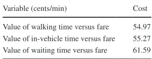
reCoMMenDeD valueS

Main valuations

The final recommended values are summarized in cents per minute across a number of tables: Table 10 shows the values for cars and motorcycles, Table 11 for taxis, Table 12 for buses and MRT, and Table 13 for walking (the last four rows of Table 13 are in cents per crossing). Car and motorcycle in-vehicle time values rely solely on valuations against ERP. An equity value of travel time was also calculated by using the values of in-vehicle time by mode weighted by travel conditions and by the island-wide daily mode share esti-mated from the 2012 HTS model; the VTT was 27.32 cents/min or $16.39/h. This equity value has increased from 18.11 cents/min in 2008, an increase of 51%, compared with a gross domestic product per-capita growth by just 29%. The higher VTT could be due to the increase in traffic congestion on the road network and passenger crowding on the public transport system, in which improved survey and modeling methodology can also have affected the values.

values of risk reduction

In terms of the recommended values of risk reduction (VRRs) for different types of accidents, those coming from CA1 are believed to be more realistic, largely because of a more accurate estimate

of the exposure risk. This finding would lead to a VRR for a fatal-ity of 4,052,123.50 Singapore dollars (S$1 = $.72 in June 2017). However, the corresponding values for serious and minor injuries (S$16,808.39 and S$52.68) are very low, possibly suggesting that respondents were focused on the number of fatalities. Ratios of 13% (for serious injury) and 1% for minor injury were obtained from the U.S. Department of Transportation (21) and applied to the VRR for fatalities to derive the VRR for serious and minor injuries, respectively. This calculation leads to the results in Table 9, which also shows a comparison against 2008 values and values from other developed countries. Although the U.S. value is in the upper range and the 2008 Singapore value is on the lower side, overall the recommended VRRs for Singapore are sensible and within an accepted range.

ConCluSionS

The work carried out to update a large number of WTP measures used in transport policy and infrastructure scheme appraisal in Singapore is summarized. The work used a distinctly large sam-ple (relative to the population) and covered a wide variety of modes and variables. The work also pushed the methodological boundaries by using mixed logit models with a full specification of heterogeneity.

The values from the analysis are in line with expectations in terms of relationships across modes (showing evidence of self-selection) as well as across journey components (e.g., effects of crowding and congestion). Insights can be gained into differences across modes in

TABLE 9 Comparison of Risk Reduction Valuations with International Results

Singapore Australiaa _UKb _{United States}c

Type of Injury (2015 $) (2008 $) (2007 $) (2014 $) (2015 $)

Fatality 4,052,124 1,874,000 6,579,854 3,580,305 12,690,000 Serious injury 526,776 243,600 320,532 402,326 1,332,450 Minor injury 40,521 18,740 17,098 31,015 38,070

a_{Hensher et al. (19).}

b_{UK Department for Transport (20).} c_{U.S. Department of Transportation (21).}

TABLE 10 Recommended Values for Cars and Motorcycles

Cost

Variable (cents/min) Car Motorcycle

Value of free-flow time versus ERP 34.32 21.20 Value of light congestion time versus ERP 36.58 24.91 Value of heavy congestion time versus ERP 46.38 24.92 Value of weighted travel time versus ERP 36.80 23.02 Value of walking time versus parking cost 36.39 na Value of queueing time versus parking cost 32.62 na Value of searching time versus parking cost 40.02 na

Note: na = not applicable.

TABLE 8 Implied Values of Risk Reduction for Accident Games for Cars and Pedestrians

Implied Value of Risk Reduction

Variable

Per Average Reported Distance (18,850 km)

Per Presented Risks (500 km/year)

terms of the relationship between congestion levels (e.g., a bigger effect for car than motorcycle) and crowding (a bigger effect for bus than MRT).

This work uncovered extensive amounts of random heterogeneity in valuations across respondents and showed clear advantages over models assuming homogeneous preferences. Interestingly, it was not possible to link much of these results to observed respondent characteristics, though some insights were gained from posterior analysis. This finding suggests that, at least with this sample, much of the heterogeneity relates to intrinsic preferences rather than differ-ences in sociodemographics. In this context, the representativeness of the sample is of crucial importance, but with the use of posterior

estimates, the possibility of course also remains open for reweighting of results.

The valuations are overall substantially higher than those from the 2008 LTA study. Although some of these findings can be attributed to changes in the transport system and increased congestion and crowding, the use of more advanced survey design and modeling approaches may also play a role. This update is thus of high impor-tance to ensure continued reliability of the cost–benefit appraisal work conducted by LTA. This study also uncovered differences in VTT measures depending on which cost attribute is used (e.g., ERP versus petrol) and it is recommended that the core values for car and motorcycle be based on ERP.

Finally, this study has put forward a different approach for SC surveys for safety; especially in the context of small areas with a low number of fatalities, the approach seems preferable to a route-based approach.

aCknoWleDgMent

The first author acknowledges the support of the European Research Council through a consolidator grant for some additional analysis.

reFerenCeS

1. Accent Marketing and Research and Hague Consulting Group. The

Value of Time on UK Roads. AHCG, The Hague, Netherlands, 1996. 2. Hess, S., A. Daly, T. Dekker, M. Ojeda Cabral, and R. P. Batley.

A Framework for Capturing Heterogeneity, Heteroskedasticity, Non-Linearity, Reference Dependence, and Design Artefacts in Value of Time Research. Transportation Research Part B: Methodological, Vol. 96, Issue C, 2017, pp. 126–149.

3. Börjesson, M., and J. Eliasson. Experiences from the Swedish Value of Time Study. Transportation Research Part A: Policy and Practice, Vol. 59, 2014, pp. 144–158. https://doi.org/10.1016/j.tra.2013.10.022. 4. Fosgerau, M., K. Hjorth, and S. Lyk-Jensen. The Danish Value of Time

Study: Final Report. Danish Transport Research Institute, Copenhagen, 2007.

5. Update of RUC Unit Values to June 2005. Austroads Publications Online, 2006. https://www.onlinepublications.austroads.com.au/items /AP-T70-06.

6. Rose, J. M., and M. C. J. Bliemer. Stated Choice Experimental Design Theory: The Who, the What, and the Why. In Handbook of Choice

Modelling (S. Hess and A. Daly, eds.), Edward Elgar, Cheltenham, United Kingdom, 2014, pp. 152–177. https://doi.org/10.4337/978178 1003152.00013.

7. Update of Economic Evaluation Parameters. Final Report. LTA, Singapore, 2009.

8. Bliemer, M. C. J., J. M. Rose, and C. Chorus. Dominance in Stated Choice Surveys and Its Impact on Scale in Discrete Choice Models. In Proceedings of the International Conference on Transport Survey

Methods, Leura, Australia, 2014.

9. Hensher, D. A., J. M. Rose, J. D. Ortúzar, and L. I. Rizzi. Estimating the Value of Risk Reduction for Pedestrians in the Road Environment: An Exploratory Analysis. Journal of Choice Modelling, Vol. 4, No. 2, 2011, pp. 70–94. https://doi.org/10.1016/S1755-5345(13)70058-7. 10. Train, K. E. Discrete Choice Methods with Simulation, 2nd ed. Cambridge

University Press, Cambridge, Mass., 2009. https://doi.org/10.1017 /CBO9780511805271.

11. Fosgerau, M., and M. Bierlaire. Discrete Choice Models with Multi-plicative Error Terms. Transportation Research Part B: Methodologi­

cal, Vol. 43, No. 5, 2009, pp. 494–505. https://doi.org/10.1016/j.trb .2008.10.004.

12. Daly, A. J., S. Hess, and K. E. Train. Assuring Finite Moments for Will-ingness to Pay in Random Coefficients Models. Transportation, Vol. 39, No. 1, 2012, pp. 19–31. https://doi.org/10.1007/s11116-011-9331-3.

TABLE 11 Recommended Values for Taxis

Variable (cents/min) Cost

Value of walking time versus fare 54.97 Value of in-vehicle time versus fare 55.27 Value of waiting time versus fare 61.59

TABLE 13 Recommended Values for Walking

Variable Cost

Value of uncovered walking time (cents/min) 15.47 Value of covered walking time (cents/min) 5.71 Value of crossing time (cents/min) 10.79 WTP for avoiding covered bridge with lift versus

air-conditioned underpass (cents/crossing) 13.56 WTP for avoiding covered bridge without lift

versus air-conditioned underpass (cents/crossing)

24.68

WTP for avoiding uncovered bridge without lift

versus air-conditioned underpass (cents/crossing) 52.11 WTP for avoiding road crossing versus

air-conditioned underpass (cents/crossing) 13.96

TABLE 12 Recommended Values for Buses and MRT

Cost

Variable (cents/min) Bus MRT

Value of walking time 15.96 22.83 Value of waiting time 15.06 17.00 Value of interchanges (cents/interchange) 40.82 68.16 Value of in-vehicle time, seated, with empty seats 10.67 17.39 Value of in-vehicle time, seated, quite packed 10.88 17.78 Value of in-vehicle time, seated, completely packed 13.01 18.01 Value of in-vehicle time, standing, quite packed 16.55 22.08 Value of in-vehicle time, standing, completely packed 17.01 24.50 Value of in-vehicle time weighted by crowding

conditions

11.73 20.71

90 Transportation Research Record 2664

13. Train, K., and M. Weeks. Discrete Choice Models in Preference Space and Willingness-to-Pay Space. In Application of Simulation Methods

in Environmental and Resource Economics (R. Scarpa and A. Alberini, eds.), Springer Publisher, Dordrecht, Netherlands, 2005, pp. 1–16. https://doi.org/10.1007/1-4020-3684-1_1.

14. Hess, S., and J. M. Rose. Can Scale and Coefficient Heterogeneity Be Separated in Random Coefficients Models? Transportation, Vol. 39, No. 6, 2012, pp. 1225–1239. https://doi.org/10.1007/s11116-012-9394-9. 15. RSGHB: Functions for Hierarchical Bayesian Estimation: A Flexible

Approach. Resource Systems Group, Inc., White River Junction, Vermont, 2015. https://cran.r-project.org/web/packages/RSGHB/index.html. 16. Hess, S., M. Bierlaire, and J. W. Polak. Estimation of Value of

Travel-Time Savings Using Mixed Logit Models. Transportation Research

Part A: Policy and Practice, Vol. 39, No. 2–3, 2005, pp. 221–236. https:// doi.org/10.1016/j.tra.2004.09.007.

17. Börjesson, M., M. Fosgerau, and S. Algers. Catching the Tail: Empirical Identification of the Distribution of the Value of Travel Time. Trans­

portation Research Part A: Policy and Practice, Vol. 46, No. 2, 2012, pp. 378–391. https://doi.org/10.1016/j.tra.2011.10.006.

18. Navrud, S., Y. Trædal, A. Hunt, A. Longo, A. Greßmann, C. Leon, R. Espino Espino, R. Markovits-Somogyi, and F. Meszaros. HEATCO:

Developing Harmonised European Approaches for Transport Costing and Project Assessment. TNO, Netherlands, 2005. http://heatco.ier .uni-stuttgart.de.

19. Hensher, D. A., J. M. Rose, J. D. Ortúzar, and L. I. Rizzi. Estimating the Willingness to Pay and Value of Risk Reduction for Car Occupants in the Road Environment. Transportation Research Part A: Policy and

Practice, Vol. 43, No. 7, 2009, pp. 692–707. https://doi.org/10.1016 /j.tra.2009.06.001.

20. UK Department for Transport. Accident and Casualty Costs. London, 2013. https://www.gov.uk/government/statistical-data-sets/ras60-average -value-of-preventing-road-accidents.

21. Guidance on Treatment of the Economic Value of a Statistical Life (VSL)

in U.S. Department of Transportation Analyses: 2015 Adjustment. U.S. Department of Transportation, June 17, 2015.

The views expressed in this paper are those of the authors and do not necessarily reflect the official position of the Land Transport Authority or of the Government of Singapore. Any remaining errors are those of the authors alone.