Properties of a general quaternion-valued gradient operator and its applications to signal processing

and its applications to signal processing

.

White Rose Research Online URL for this paper:

http://eprints.whiterose.ac.uk/97387/

Version: Accepted Version

Article:

Jiang, M-D., Li, Y. and Liu, W. orcid.org/0000-0003-2968-2888 (2016) Properties of a

general quaternion-valued gradient operator and its applications to signal processing.

Frontiers of Information Technology & Electronic Engineering, 17 (2). pp. 83-95. ISSN

2095-9184

https://doi.org/10.1631/FITEE.1500334

[email protected] https://eprints.whiterose.ac.uk/ Reuse

Unless indicated otherwise, fulltext items are protected by copyright with all rights reserved. The copyright exception in section 29 of the Copyright, Designs and Patents Act 1988 allows the making of a single copy solely for the purpose of non-commercial research or private study within the limits of fair dealing. The publisher or other rights-holder may allow further reproduction and re-use of this version - refer to the White Rose Research Online record for this item. Where records identify the publisher as the copyright holder, users can verify any specific terms of use on the publisher’s website.

Takedown

If you consider content in White Rose Research Online to be in breach of UK law, please notify us by

Properties of a General Quaternion-Valued Gradient

Operator and Its Application to Signal Processing

Mengdi Jiang

a

, Yi Li

b

, Wei Liu

a

a_{Communications Research Group, Department of Electronic and Electrical Engineering}

University of Sheffield, Sheffield, S1 3JD, United Kingdom {mjiang3, w.liu}@sheffield.ac.uk

b_{School of Mathematics and Statistics}

University of Sheffield, Sheffield, S3 7RH, United Kingdom

[email protected]

Abstract—The gradients of a quaternion-valued function are often required for quaternionic signal processing algorithms. The HR gradient operator provides a viable framework and has found a number of applications. However, the applications so far have been mainly limited to real-valued quaternion functions and linear quaternion-valued functions. To generalize the operator to nonlinear quaternion functions, we define a restricted version of the HR operator, which comes in two versions, the left and the right ones. We then present a detailed analysis of the properties of the operators, including several different product rules and chain rules. Using the new rules, we derive explicit expressions for the derivatives of a class of regular nonlinear quaternion-valued functions, and prove that the restricted HR gradients are consistent with the gradients in real domain. As an application, the derivation of the least mean square algorithm and a nonlinear adaptive algorithm is provided. Simulation results based on vector sensor arrays are presented as an example to demonstrate the effectiveness of the quaternion-valued signal model and the derived signal processing algorithm.

I. INTRODUCTION

Quaternion calculus has been introduced in signal process-ing with application areas involvprocess-ing three or four-dimensional signals, such as color image processing [1]–[5], vector-sensor array systems [6]–[11] and wind profile prediction [12]. Several quaternion-valued adaptive filtering algorithms have been proposed in [10], [11], [13], [14]. Notwithstanding the advantages of the quaternionic algorithms, extra care have to be taken in their developments, in particular when the derivatives of quaternion-valued functions are involved, due to the fact that quaternion algebra is non-commutative. A so-called HR gradient operator was proposed in [15] and the interesting formulation appears to provide a general and flex-ible framework that could potentially have wide applications. However, it has only been applied to real-valued functions and linear quaternion-valued functions. In order to consider more general quaternion-valued functions, we propose a pair of restricted HR gradient operators, the left and the right restricted HR gradient operators, based on the previous work on the HR gradient operator [15] and our recent work [12].

To summarize, we make the following main contributions. Firstly, we give a detailed derivation of the relation between the gradients and the increment of a quaternion function, highlighting the difference between the left and the right gradients due to the non-commutativity of quaternion algebra.

Secondly, we document several properties of the operators that have not been reported before, in particular several different versions of product rules and chain rules. Thirdly, we derive a general formula for the restricted HR derivatives of a wide class of regular quaternion-valued nonlinear functions, among which are the exponential, logarithmic, and the hyperbolic tangent functions. Finally, we prove that the restricted HR gra-dients are consistent with the usual definition for the gradient of a real function of a real variable. Its application to the derivation of quaternion-valued least mean squares (QLMS) adaptive algorithm and a nonlinear adaptive algorithm based on the hyperbolic tangent function is also briefly discussed. As an example for quaternion-valued signal processing, we will consider the reference signal based adaptive beamform-ing problem for vector sensor arrays consistbeamform-ing of multiple crossed-dipoles and provide some simulation results.

The paper is organised as follows. The restricted HR gradient operator is developed in Sec. II, with its properties and rules introduced in Sec. III. Explicit expressions for the derivatives for a wide range of functions are derived in Sec. IV and results for the right restricted HR operator are summarised in Sec. V. The increment of a general quaternion function is discussed in Sec. VI, followed by its two applications. The quaternion-valued adaptive beamforming example is provided in Sec. VII and conclusions are drawn in Sec. VIII.

II. THE RESTRICTEDHRGRADIENT OPERATORS

A. Introduction of quaternion

Quaternion is a non-commutative extension of complex number. A quaternion q is composed of four parts, i.e.,

q = qa +qbi+qcj+qdk, whereqa is the real part, which

is also denoted as R(q). The other three terms constitute the imaginary part I(q).i,j andk are the three imaginary units, which satisfy the following rules for multiplication: ij =k,

jk=i,ki=j,i2_=j2_=k2_{=−1, and}

ij=−ji, ki=−ik, kj =−jk. (1)

Letv =|I(q)| and ˆv=I(q)/v, the quaternion q can also

be written asq=qa+vvˆ.vˆ is a pure unit quaternion, which

has the convenient propertyvˆ2:= ˆvvˆ=−1. The quaternionic

conjugate ofqisq∗

=qa−qbi−qcj−qdk, orq∗=qa−vvˆ. It is

easy to show thatqq∗ =q∗

q=|q|2_{, and henceq}−1_=q∗

/|q|2_.

B. Definition of the restricted HR gradient operators

Let f : H → H be a quaternion-valued function of a quaternion q, where H is the non-commutative algebra of quaternions. We use the notationf(q) =fa+fbi+fcj+fdk,

where fa, ..., fd are the components of f. f can also be

viewed as a function of the four components of q, i.e.,f =

f(qa, qb, qc, qd). In this viewf is a quaternion-valued function

onR4_{: f :R}4_{→H. To express the four real components of}

q, it is convenient to use its involutions qν _{:= −νqν where}

ν∈ {i, j, k} [16]. Explicitly, we have

qi=−iqi=qa+qbi−qcj−qdk, (2)

qj =−jqj =qa−qbi+qcj−qdk, (3)

qk =−kqk=qa−qbi−qcj+qdk. (4)

The real components can be recovered by

qa=

1 4(q+q

i_+qj_+qk_{), q} b =

1 4i(q+q

i_−qj_−qk_{), (5)}

qc= 1

4j(q−q

i_+qj_−qk_{), q} d= 1

4k(q−q

i_−qj_+qk_).

(6)

Two useful relations are

q∗

= 1 2(q

i_+qj_+qk_{−q), q+q}i_+qj_+qk_{= 4R(q).}

(7)

A so-called HR gradient of f(q) was introduced in [15], which has been applied to real-valued functions and linear quaternion-valued functions. In order to find the gradients of more general quaternion-valued functions, we follow a similar approach to propose a ‘restricted’ HR gradient operator (some of the derivation was first presented in [12]). To motivate the definitions, we consider the differentialdf(q)with respect to differentialdq:=dqa+dqbi+dqcj+dqdk. We observe that

df=dfa+idfb+jdfc+kdfd, where

dfa= ∂fa

∂qa

dqa+∂fa

∂qb

dqb+∂fa

∂qc

dqc+∂fa

∂qd

dqd. (8)

We have dqa = (dq+dqi+dqj+dqk)/4 according to (5).

Making use of this and similar expressions for dqb,dqc and

dqd, we find an expression fordfa in terms of the differentials

dq,dqi_,dqj _anddqk_{. Repeating the calculation foridf} b,jdfc

andkdfd, we finally arrive at

df =Ddq+Didqi+Djdqj+Dkdqk (9)

where

D:= 1

4 (_∂f

∂qa

− ∂f

∂qb

i− ∂f

∂qc

j− ∂f

∂qd

k

)

, (10)

Di:= 1

4 ( ∂f ∂qa − ∂f ∂qb

i+ ∂f

∂qc

j+ ∂f

∂qd

k

)

, (11)

Dj:=

1 4 ( ∂f ∂qa + ∂f ∂qb

i− ∂f

∂qc

j+ ∂f

∂qd

k

)

, (12)

Dk:=

1 4 (_∂f ∂qa + ∂f ∂qb

i+ ∂f

∂qc

j− ∂f

∂qd

k

)

. (13)

More details are given in Appendix A. Thus one may define the partial derivatives off(q)as follows:

∂f

∂q :=D,

∂f

∂qi :=Di,

∂f

∂qj :=Dj,

∂f

∂qk :=Dk. (14)

Introducing operators ∇q := (∂/∂q, ∂/∂qi, ∂/∂qj, ∂/∂qk),

and ∇r := (∂/∂qa, ∂/∂qb, ∂/∂qc, ∂/∂qd), equations (10-14)

may be written as

∇qf =∇rf JH (15)

where the Jacobian matrix

J = 1

4 

  

1 i j k

1 i −j −k

1 −i j −k

1 −i −j k



  

(16)

and JH _{is the Hermitian transpose ofJ [15]. UsingJJ}H ₌

JH_{J = 1/4 [17], we may also write}

∇qf J = 1

4∇rf, (17)

which is the inverse formulae for the derivatives.

We call the gradient operator defined by (15) the restricted HR gradient operator. The operator is closely related to the HR operator introduced in [15]. However, in the original definition of the HR operator, the Jacobian J appears on the left-hand side of∇rf, whereas in our definition it appears on the right

(as the Hermitian transpose).

The differential df is related to∇qf by

df= ∂f

∂qdq+

∂f

∂qidq

i₊ ∂f

∂qjdq

j₊ ∂f

∂qkdq

k_{. (18)}

Due to the non-commutativity of quaternion products, the order of the factors in the products of the above equation (as well as equations (10-13)) can not be swapped. In fact, one may call the above operator the left restricted HR gradient operator. As is shown in Appendix A, one may also define a right restricted HR gradient operator by

(∇R

qf)T :=J ∗

(∇rf)T, (19)

where

∇Rq := (∂R/∂q, ∂R/∂qi, ∂R/∂qj, ∂R/∂qk),

and

∂R_f

∂q := 1 4 ( ∂f ∂qa

−i∂f

∂qb

−j∂f

∂qc

−k∂f

∂qd

)

, (20)

∂R_f

∂qi :=

1 4

(_∂f

∂qa

−i∂f

∂qb

+j∂f

∂qc

+k∂f

∂qd

)

, (21)

∂R_f

∂qj :=

1 4

(

∂f

∂qa

+i∂f

∂qb

−j∂f

∂qc

+k∂f

∂qd

)

, (22)

∂R_f

∂qk :=

1 4

(_∂f

∂qa

+i∂f

∂qb

+j∂f

∂qc

−k∂f

∂qd

)

. (23)

The right restricted HR gradient operator is related to the differential df by

df =dq∂

R_f

∂q +dq

i∂Rf

∂qi +dq

j∂Rf

∂qj +dq

k∂Rf

In general, the left and right restricted HR gradients are not the same. For example, even for the simplest linear function

f(q) =q0qwithq0∈H a constant, we have

∂q0q

∂q =q0,

∂R_q

0q

∂q =R(q0). (25)

However, we will show later that the two gradients coincide for a class of functions. In particular, they are the same for real-valued quaternion functions.

The relation between the gradients and the differential is an important ingredient of gradient-based methods, which we will discuss further later.

III. PROPERTIES AND RULES OF THE OPERATOR

We will now focus on the left restricted HR gradient and simply call it the restricted HR gradient unless stated otherwise. It can be easily calculated from the definitions, that

∂q

∂q = 1,

∂qν

∂q = 0,

∂q∗

∂q =−

1

2, (26)

whereν ∈ {i, j, k}. However, in order to find the derivatives for more complex quaternion functions, it is useful to first establish the rules of the gradient operators. We will see that some of the usual rules do not apply due to the non-commutativity of quaternion products.

1) Left-linearity: for arbitrary constant quaternions α and

β, and functions f(q)andg(q), we have

∂(αf+βg)

∂qν =α

∂f

∂qν +β

∂g

∂qν (27)

forν∈ {1, i, j, k}withq1_{:=q. However, linearity does}

not hold for right multiplications, i.e., in general

∂f α

∂q ̸=

∂f

∂qα. (28)

This is because, according to the definition (10),

∂f α

∂q =

1 4

∑

(φ,γ)

∂f

∂qφ

αγ (29)

for(φ, γ)∈ {(a,1),(b,−i),(c,−j),(d,−k)}. However,

αγ ̸= γα in general. Therefore it is different from

(∂f /∂q)α, which is

1 4

(

∂f

∂qa

− ∂f

∂qb

i− ∂f

∂qc

j− ∂f

∂qd

k

)

α. (30)

2) The first product rule: the following product rule holds:

∇q(f g) =f∇qg+ [(∇rf)g]JH. (31)

For example,

∂f q

∂q =f

∂g

∂q+

1 4

(_∂f

∂qa

g− ∂f

∂qb

gi− ∂f

∂qc

gj− ∂f

∂qd

gk

)

.

(32) Thus the product rule in general is different from the usual one.

3) The second product rule: However, the usual product rule applies to differentiation with respect to real vari-ables, i.e.,

∂f g

∂qφ

= ∂f

∂qφ

g+f ∂g

∂qφ

(33)

forφ=a, b, c, ord.

4) The third product rule: The usual product rule also applies if at least one of the two functions f(q) and

g(q)is real-valued, i.e.,

∂f q

∂q =f

∂g

∂q +

∂f

∂qg. (34)

5) The first chain rule: For a composite function f(g(q)),

g(q) :=ga+gbi+gcj+gdkbeing a quaternion-valued

function, we have the following chain rule [17]:

∇qf = (∇gqf)M (35)

where∇g

q := (∂/∂g, ∂/∂gi, ∂/∂gj, ∂/∂gk)andM is a

4×4 matrix with elementMµν =∂gµ/∂qν for µ, ν∈

{1, i, j, k} and gµ _{= −µgµ (g}1 _{is understood as the}

same asg). Explicitly, we may write

∂f

∂qν =

∑

µ

∂f

∂gµ

∂gµ

∂qν. (36)

The proof is outlined in Appendix C.

6) The second chain rule: The above chain rule uses g

and its involutions as the intermediate variables. It is sometimes convenient to use the real components ofg

for that purpose instead. In this case, the following chain rule may be used:

∇qf = (∇grf)O (37)

whereO is a 4×4 matrix with entryOφν =∂gφ/∂qν

with φ ∈ {a, b, c, d} and ν ∈ {1, i, j, k}, and ∇g

r :=

(∂/∂ga, ∂/∂gb, ∂/∂gc, ∂/∂gd). Explicitly, we have

∂f

∂qν =

∑

φ

∂f

∂gφ

∂gφ

∂qν. (38)

7) The third chain rule: if the intermediate function g(q)

is real-valued, i.e.,g=ga, then from the second chain

rule, we obtain

∂f

∂qν =

∂f ∂g

∂g

∂qν. (39)

8) f(q)is not independent ofqi_,qj_orqk_{in the sense that,}

in general,

∂f(q)

∂qi ̸= 0,

∂f(q)

∂qj ̸= 0,

∂f(q)

∂qk ̸= 0. (40)

This can be illustrated by f(q) = q2_{. Using the first}

product rule (equation (31)), we have

∂q2

∂qi =q

∂q

∂qi +

1 4

∑

(φ,ν)

∂q

∂qφ

qν

for (φ, ν)∈ {(a,1),(b, i),(c,−j),(d,−k)}. It can then be shown that

∂q2

∂qi =qbi,

∂q2

∂qj =qcj,

∂q2

∂qk =qdk. (41)

This property demonstrates the intriguing difference between the HR derivative and the usual derivatives, although we can indeed show that

∂q

One implication of this observation is that, for a nonlin-ear algorithm involving simultaneously more than one gradients ∂f /∂qν_{, we have to take care to include all}

the terms.

IV. RESTRICTEDHRDERIVATIVES FOR A CLASS OF REGULAR FUNCTIONS

Using the above operation rules, we may find explicit expressions for the derivatives for a whole range of functions. We first introduce the following lemma:

Lemma 1. The derivative of the power functionf(q) = (q−

q0)n, with integernand constant quaternion q0, is

∂f(q)

∂q =

1 2

(

nq˜n−1₊q˜n−q˜

∗n

˜

q−q˜∗

)

, (43)

withq˜=q−q0.

Remark. The division in(˜qn_−q˜∗n_)/(˜q−q˜∗

)is understood as

(˜qn_−q˜∗n_)(˜q−q˜∗

)−1 _or(˜q−q˜∗

)−1_(˜qn_−q˜∗n_{)which are the}

same since the two factors commute. The division operations in what follows are understood in the same way.

Proof:The lemma is obviously true forn= 0. Letn≥1, we apply the first product rule, and find

∂(q−q0)n

∂q = ˜q

∂q˜n−1

∂q +R(˜q

n−1₎

(44)

where R(˜qn−1_{) is the real part of q˜}n−1_{. We then obtain by}

induction

∂(q−q0)n

∂q =

n−1 ∑

m=0 ˜

qmR(˜qn−1−m_).

(45)

UsingR(˜qn−1−m_{) =} 1 2(˜qn

−1−m_{+ ˜q}∗(n−1−m)_{), the}

summa-tions can be evaluated explicitly, leading to equation (43).

Forn <0, we use the recurrent relation

∂((q−q0)−n)

∂q = ˜q

−1 [

∂q˜−(n−1)

∂q −R(˜q

−n₎ ]

(46)

and the result

∂(q−q0)−1

∂q =−q˜

−1_R(˜q−1_).

(47)

Equation (43) is proven by using induction as forn >0. More details are given in Appendix B.

Theorem 1. Assuming f : H → H admits a power series representationf(q) :=g(˜q) :=∑∞

n=−∞anq˜

n_{, witha} n being

a quaternion constant and q˜ = q−q0, for R1 ≤ |q˜| ≤ R2

withR1, R2>0being some constants, then

∂f(q)

∂q =

1 2 [

f′

(q) + (g(˜q)−g(˜q∗

))(˜q−q˜∗ )−1]

, (48)

wheref′

(q)is the derivative in the usual sense, i.e.,

f′

(q) := ∞ ∑

n=−∞

nanq˜n−1=

∞ ∑

n=−∞

nan(q−q0)n−1. (49)

Proof: Using Lemma 1 and the left-linearity of HR gradients, we have

∂f

∂q =

1 2

∞ ∑

n=−∞

an[nq˜n−1+ (˜qn−q˜∗n)(˜q−q˜∗)−1]

=f′ (q) +1

2 [ ∞

∑

n=∞

an(˜qn−q˜

∗n₎ ]

(˜q−q˜∗ )−1

=1 2[f

′

(q) + (g(˜q)−g(˜q∗

))(˜q−q˜∗ )−1_],

proving the theorem.

The functionsf(q)form a class of regular functions onH. A full discussion of such functions is beyond the scope of this paper. However, we note that a similar class of functions have been discussed in [18]. A parallel development for the former is possible, and will be the topic of a future paper. Meanwhile, we observe that many useful elementary functions satisfy the conditions in Theorem 1. To illustrate the application of the theorem, we list below the derivatives of a number of such functions.

Example 1. Exponential function f(q) =eq _has

representa-tion

eq :=

∞ ∑

n=0

qn

n!. (50)

Applying Theorem 1 with an= 1/n!andq0= 0, we have

∂eq

∂q =

1 2

(

eq+e

q_−eq∗

q−q∗

)

. (51)

Making use of eq _=eqa+ˆvv =eqaeˆvv = eqa(cosv+ ˆvsinv)

with the representation of q = qa + ˆvv and ˆv2 = −1,

respectively, we have

∂eq

∂q =

1 2 (

eq+eqa

v−1_sinv)

. (52)

Example 2. The logarithmic functionf(q) = lnq has repre-sentation

lnq= ∞ ∑

n=1

(−1)n−1

n (q−1)

n_.

(53)

withan= (−1)n−1/nandq0= 1. Sinceq0 is a real number,

g(˜q∗

) =f(q∗

). Therefore, we have from Theorem 1

∂lnq

∂q =

1 2

(

q−1₊lnq−lnq

∗

q−q∗

)

. (54)

Using representation lnq = ln|q| + ˆvarccos(q_a/|q|), the

expression can be simplified as

∂lnq

∂q =

1 2

(

q−1₊1

v arccos

qa

|q| )

, (55)

wherev=|I(q)|.

Example 3. Hyperbolic tangent function f(q) = tanhq is defined as

tanhq:= e q_−e−q

eq_+e−q =q−

q3

3 + 2q5

Therefore, Theorem 1 applies. On the other hand, using the relationeq_=eqa(cosv+ ˆ

vsinv), we can show that

tanhq= 1 2

sinh 2qa+ ˆvsin 2v sinh2qa+ cos2v

. (57)

Then the second term in the expression given by Theorem 1 can be simplified. The final expression can be written as

∂tanhq

∂q =

1 2

(

sech2q+ v

−1_{sin 2v}

cosh 2qa+ cos 2v )

, (58)

where sechq := 1/coshq is the quaternionic hyperbolic secant function.

Remark. Apparently, the derivatives for these functions can also be found by direct calculations without resorting to Theorem 1.

We now turn to a question of more theoretical interests. Even though it might not be obvious from the definitions, the following theorem shows that the restricted HR derivative is consistent with the derivative in the real domain for a class of functions, including those in the above examples.

Theorem 2. For the function f(q) in Theorem 1, if q0 is a

real number, then

∂f(q)

∂q →f

′

(q) (59)

whenq→R(q), i.e., whenq approaches a real number. Proof: Using the polar representation, we write q˜ = |q˜|exp(ˆvθ), where θ = arcsin(v/|q˜|) is the argument of q˜

withv=|I(˜q)|. Thenq˜n _=|q˜|n_{exp(nvˆθ), and}

(˜qn_−q˜∗n_)(˜q−q˜∗

)−1₌ I(˜qn)

I(˜q) =

|q˜|n−1_sin(nθ)

sinθ . (60)

For real q0, q˜→qa−q0 andv →0 when q→R(q). There

are two possibilities. Firstly, ifqa−q0≥0, thenθ→0at the

limit. Thus,

sin(nθ) sinθ ∼

sin(nθ)

θ →n, |q˜|

n−1_→(q

a−q0)n−1. (61)

Therefore,

(˜qn_−q˜∗n_)(˜q−q˜∗

)−1_→nq˜n−1 ₍₆₂₎

and

[g(˜q)−g(˜q∗

)](˜q−q˜∗ )−1_→

∞ ∑

n=−∞

nanq˜n−1=f′(q). (63)

Thus

∂f(q)

∂q →

1 2[f

′ (q) +f′

(q)] =f′

(q). (64)

Secondly, ifqa−q0<0, thenθ→π. Thus

sin(nθ) sinθ ∼

sin(nθ)

π−θ (65)

Notesin(nθ) = sin[nπ−n(π−θ)] = (−1)n−1_{sin[n(π−θ)],}

we have

sin(nθ) sinθ ∼

(−1)n−1_{sin(n(π−θ)}

π−θ →(−1)

n−1_n.

(66)

On the other hand, in this case |q˜| → −(qa −q0), hence |q˜|n−1 _{→ (−1)}n−1_(q

a −q0)n−1. Since q˜ → qa −q0, as a

consequence, we have

(˜qn−q˜∗n_)(˜q−q˜∗

)−1_→nq˜n−1

(67)

which is the same as Eq. (62). The proof then follows from the first case.

The functions in above three examples all satisfy the con-ditions in Theorem 2, hence we expect Theorem 2 applies. One can easily verify by direct calculations that the theorem indeed holds.

V. THE RIGHT RESTRICTEDHRGRADIENTS

In this section, we briefly summarize the results for the right restricted HR gradients, and highlight the difference with left restricted HR gradients.

1) Right-linearity: for arbitrary quaternion constantsαand

β, and functions f(q)andg(q), we have

∂R_{(f α+gβ)}

∂qν =

∂R_f

∂qν α+

∂R_g

∂qνβ. (68)

However, linearity does not hold for left multiplications, i.e., in general

∂R_αf

∂q ̸=α

∂R_f

∂q . (69)

2) The first product rule: for the right restricted HR oper-ator, the following product rule holds:

[∇R

q(f g)]T = [(∇Rqf)g]T +J ∗

[f(∇rg)T]. (70)

The second and third product rules are the same as for the left restricted operator.

3) The first chain rule: for the composite functionf(g(q)), we have

(∇Rqf)T =MT(∇gRq f)T. (71)

4) The second chain rule becomes:

(∇Rqf)T =OT(∇grf)T. (72)

5) The third chain rule becomes

∂R_f

∂qν =

∂g

∂qν

∂f

∂g. (73)

Note that, ∂g/∂qν = ∂Rg/∂qν since g is real-valued. We thus have omitted the superscriptR. Also,∂f /∂gis a real derivative, so there is no distinction between left and right derivatives.

We can also find the right restricted HR gradients for common quaternion functions. First of all, Lemma 1 is also true for right derivatives:

Lemma 2. For f(q) = (q−q0)n with n integer and q0 a

constant quaternion, we have

∂R_f(q)

∂q =

1 2

(

nq˜n−1₊q˜n−q˜

∗n

˜

q−q˜∗

)

, (74)

Remark. To prove the lemma, we use the following recurrent relations:

∂(q−q0)n

∂q =

∂q˜n−1

∂q q˜+R(˜q

n−1₎

(75)

∂((q−q0)−n)

∂q =

[_∂q˜−(n−1)

∂q −R(˜q

−n₎ ]

˜

q−1_.

(76)

Using Lemma 2, We can prove the following result:

Theorem 3. Assuming f : H → H admits a power series representationf(q) :=g(˜q) :=∑∞

n=−∞q˜ n_a

n, withan being

a quaternion constant and q˜ = q−q0, for R1 ≤ |q˜| ≤ R2

withR1, R2>0being some constants, then

∂R_f(q)

∂q =

1 2 [

f′

(q) + (˜q−q˜∗

)−1_{(g(˜q)−g(˜q}∗ ))]

, (77)

wheref′

(q)is the derivative in the usual sense, i.e.,

f′

(q) := ∞ ∑

n=−∞

nq˜n−1_a

n= ∞ ∑

n=−∞

n(q−q0)n−1an. (78)

Note that, the functionsf(q)in Theorem 3 in general form a different class of functions than the one in Theorem 1, because in the series representationan appears on the right-hand side

of the powers. However, if an is a real number, then the two

classes of functions coincide. Therefore, we have the following result:

Theorem 4. Ifan is real, then the left and right restricted HR

gradients off(q)coincide.

Remark. As a consequence, we can see immediately the right derivatives for the exponential, logarithmic and hyperbolic tangent functions are the same as the left ones.

Apparently, Theorem 2 is also true for the right derivatives. Hence, we have:

Theorem 5. The right-restricted HR gradient is consistent with the real gradient in the sense of Theorem 2.

VI. THE INCREMENT OF A QUATERNION FUNCTION

When f(q) is a real-valued quaternion function, both left and right restricted HR gradients are coincident with the HR gradients. Besides, we have

∂R_f

∂qν =

∂f

∂qν =

(

∂f ∂q

)ν

, (79)

where ν ∈ i, j, k. Thus only ∂f /∂q is independent. As a consequence (see also [15]),

df=∑

ν

∂f

∂qνdq

ν ₌∑

ν (

∂f ∂q

)ν

dqν

=∑

ν (

∂f

∂qdq

)ν = 4R

(

∂f

∂qdq

)

, (80)

where equation (79) has been used. Hence,−(∂f /∂q)∗

gives the steepest descent direction for f, and the increment is determined by ∂f /∂q.

On the other hand, iff is a quaternion-valued function, the increment will depend on all four derivatives. Takingf(q) =

q2 _{as an example, we have (see equations (41) and (43))}

dq2= (q+qa)dq+qbidqi+qcjdqj+qdkdqk, (81)

even thoughf(q)appears to be independent ofqi_,qj _andqk_.

It can be verified that the above expression is the same as the differential form given in terms ofdqa,dqb,dqcanddqd. Thus

it is essential to include the contributions from∂f /∂qi _etc.

We also note that, if the right gradient is used consistently, the same increment would result, since the basis of the definitions is the same, namely, the differential form in term of dqa,dqb,dqc anddqd.

A. Quaternion-valued LMS algorithm

As an application, we now apply the quaternion-valued re-stricted HR gradient operator to develop the QLMS algorithm. Different versions of the QLMS algorithm have been derived in [10], [12], [14]. However, with the rules we have derived, some of the calculations can be simplified, as we will be showing below.

In terms of a standard adaptive filter, the output y[n] and error e[n]can be expressed as

y[n] =wT[n]x[n], e[n] =d[n]−wT[n]x[n], (82)

where w[n] is the adaptive weight coefficient vector, d[n]

the reference signal, and x[n] the input sample vector. The conjugate e∗

[n] of the error signale[n]is

e∗

[n] =d∗

[n]−xH[n]w∗

[n]. (83)

The cost function is defined asJ[n] =e[n]e∗

[n]which is real-valued. According to the discussion above and [15], [19], the conjugate gradient (∇wJ[n])∗ gives the maximum steepness

direction for the optimization surface. Therefore it is used to update the weight vector. Specifically,

w[n+ 1] =w[n]−µ(∇wJ[n]) ∗

, (84)

whereµis the step size. To find∇wJ, we use the first product

rule:

∇wJ =

∂e[n]e∗

[n]

∂w

= e[n]∂e ∗

[n]

∂w +

1 4(

∂e[n]

∂wa e

∗

[n]−∂e[n]

∂wb e

∗ [n]i

−∂e[n]

∂wc

e∗

[n]j−∂e[n]

∂wd

e∗

[n]k) (85)

After some algebra, we find∇wJ[n] =−1₂x[n]e∗[n], which

leads to the following update equation for the QLMS algorithm

w[n+ 1] =w[n] +µ(e[n]x∗

[n]). (86)

B. Quaternion-valued nonlinear adaptive algorithm

tanh(y[n]) = tanh(wT[n]x[n]). The cost function is given byJ[n] =e[n]e∗

[n], withe[n] =d[n]−tanh(wT[n]x[n]). Using the product rules in (85) and chain rules, and letting

y[n] =wT[n]x[n], we have

∂e∗

[n]

∂w[n] =−(

∂tanh(y∗ [n])

∂(y∗_[n])

a

∂(y∗

[n])a

∂w[n]

+∂tanh(y ∗

[n])

∂(y∗_[n])

b

∂(y∗

[n])b

∂w[n] +

∂tanh(y∗ [n])

∂(y∗_[n])

c

∂(y∗

[n])c

∂w[n]

+∂tanh(y ∗

[n])

∂(y∗_[n])

d

∂(y∗

[n])d

∂w[n] ). (87)

Let u = |I(y)| and uˆ = I(y)/u. Then the quaternion y =

ya+I(y)can also be written asy=ya+uu.ˆ uˆis a pure unit

quaternion. Finally, the gradient can be expressed as follows by using (57)

∇wJ[n] =

1

4(sinh2ya+ cos2u)2

·(

(2 sin 2u(easin2ya+ sin 2u(eˆu)a)

+ (cosu−sinu

u )(sinh

2_y

a+ cos2u)(eˆu)a)xˆu

+ea((sinh2ya+ cos2u)(sinu

u −4 cosh 2ya)

+ sinh 2ya(sinh2ya−sin 2u(euˆ)a))x

+ 2sinu

u (sinh

2_y

a+ cos2u)(exa+e ∗

x)a) )

(88)

Substituting the above result into Eq. (84) we can then obtain the update equation for the nonlinear adaptive algorithm.

On the other hand, if we use the series representation of

tanh(q), we can obtain another form of the gradient function and the corresponding update equation becomes

w[n+ 1] =

w[n]+1 2µ

∞ ∑

m=0 m−1

∑

r=0

am(xH[n]w∗[n])m−1−r

·e[n](xH[n]w∗ [n])r_x∗

[n], (89)

where am is the coefficient in the series representation of tanh(y[n]), i.e., tanh(y[n]) = ∑∞

m=0am(y[n])m. It can be

shown that if the items in the gradient part of the above expression are commutative, it will be reduced to the same form as in the real or complex domain.

VII. APPLICATION TO ADAPTIVE BEAMFORMING BASED ON VECTOR SENSOR ARRAYS

As an example for the application of quaternion-valued signal processing, we here consider the reference signal based adaptive beamforming problem for vector sensor arrays con-sisting of multiple crossed-dipoles, where the earlier derived QLMS algorithm can be employed for beamforming.

A. Vector sensor arrays with a quaternion model

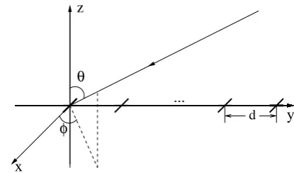
A general structure for a uniform linear array (ULA) with

M crossed-dipole pairs is shown in Fig. 1, where these pairs are located along the y-axis with an adjacent distanced, and at each location the two crossed components are parallel to the

d

...

θ

φ

y

z

[image:8.595.321.529.50.172.2]

x

Fig. 1. A ULA with crossed-dipoles.

x-axis and y-axis, respectively. For a far-field incident signal with a direction of arrival (DOA) defined by the anglesθand

φ, its spatial steering vector is given by

Sc(θ, φ) = [1, e−j2πdsinθsinφ/λ,

· · ·, e−j2π(M−1)dsinθsinφ/λ_]T

(90)

where λ is the wavelength of the incident signal and {·}T

denotes the transpose operation. For a crossed dipole the spatial-polarization coherent vector can be given by [11], [21], [22]

Sp(θ, φ, γ, η) =

{

[−cosγ,cosθsinγejη_{] for φ=}π 2 [cosγ,−cosθsinγejη_{] for φ=}−π

2

(91) whereγ is the auxiliary polarization angle with γ∈[0, π/2], andη∈[−π, π]is the polarization phase difference.

The array structure can be divided into two sub-arrays: one parallel to the x-axis and one to the y-axis. The complex-valued steering vector of the x-axis sub-array is given by

Sx(θ, φ, γ, η) =

{

−cosγSc(θ, φ) for φ=π₂ cosγSc(θ, φ) for φ=−₂π

(92)

and for the y-axis it is expressed as

Sy(θ, φ, γ, η) =

{

cosθsinγejη_S

c(θ, φ) forφ= π₂

−cosθsinγejη_S

c(θ, φ) forφ= −₂π

(93) Combining the two complex-valued subarray steering vec-tors together, an overall quaternion-valued steering vector with one real part and three imaginary parts can be constructed as

Sq(θ, φ, γ, η)

= ℜ{Sx(θ, φ, γ, η)}+iℜ{Sy(θ, φ, γ, η)}

+jℑ{Sx(θ, φ, γ, η)}+kℑ{Sy(θ, φ, γ, η)},

(94)

where ℜ{·} and ℑ{·} are the real and imaginary parts of a complex number/vector, respectively. Given a set of coeffi-cients, the response of the array is given by

r(θ, φ, γ, η) =wHSq(θ, φ, γ, η) (95)

[

.

.

.

+

−

.

.

.

]

]

]

]

] ]

d

[

n

n

x

M[

n

w

_M[

n

n

[

n

[

e

y

w

1

x

₁[

]

[image:9.595.93.241.54.147.2]

n

Fig. 2. Reference signal based adaptive beamforming structure.

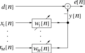
B. Reference signal based adaptive beamforming

Suppose one of the incident signals to the array is the desired one and the remaining signals are interferences. Then the aim of beamforming is to receive the desired signal while suppressing the interferences at the output of the beamformer [23]. When a reference signald[n]is available, adaptive beam-forming can be implemented by the standard adaptive filtering structure, as shown in Fig. 2, where xm[n], m = 1,· · · , M

are the received quaternion-valued input signals through the

M pairs of crossed-dipoles, and wm[n], m = 1,· · ·, M are

the corresponding quaternion-valued weight coefficients.y[n]

is the beamformer output ande[n] is the error signal

y[n] = wT[n]x[n]

e[n] = d[n]−wT[n]x[n], (96)

where

w[n] = [w1[n], w2[n],· · ·, wM[n]]T

x[n] = [x1[n], x2[n],· · · , xM[n]]T . (97)

Simulations are performed based on such an array with 16

crossed-dipoles and half-wavelength spacing using the QLMS algorithm in (86). The stepsizes µ is set to be 2×10−4_{. A}

desired signal with 20 dB signal to noise ratio (SNR) impinges from the broadside of the array (θ= 15◦

) and two interfering signals with a signal to interference ratio (SIR) of -10 dB arrive from the directions(30◦

,90◦

), and(15◦

,−90◦

), respectively. All the signals have the same polarisation of(γ, η) = (30◦

,0).

Its learning curve obtained by averaging results from 200

simulation runs is shown in Fig. 3 and the resultant beam pattern is shown in Fig. 4, where for convenience positive values ofθindicate the value rangeθ∈[0◦

, 90◦

]forφ= 90◦

, while negative values ofθ∈[−90◦

, 0◦

]indicate an equivalent range of θ ∈[0◦

, 90◦

] withφ=−90◦

. We can see that the ensemble mean square error has reached almost -30dB and two nulls have been formed successfully in the two interference directions, demonstrating the effectiveness of the quaternion-valued signal model and the derived QLMS algorithm.

VIII. CONCLUSIONS

We have proposed a restricted HR gradient operator and discussed its properties, in particular several different versions of product rules and chain rules. Using the rules that we establish, we derive a general formula for the derivative of a large class of nonlinear quaternion-valued functions. The

0 1000 2000 3000 4000 5000 6000 7000 8000 −35

−30 −25 −20 −15 −10 −5 0

Iterations

Ensemble Normalised Mean Square Error [dB]

[image:9.595.324.534.56.192.2]

QLMS

Fig. 3. Learning curve of the QLMS algorithm.

−80 −60 −40 −20 0 20 40 60 80

−60 −50 −40 −30 −20 −10 0

theta(degrees)

[image:9.595.322.539.232.370.2]

The beam pattern of array(dB)

Fig. 4. Resultant beam pattern of the QLMS algorithm.

class includes the common elementary functions such as the exponential function, the logarithmic function, among others. We also prove that, for a wide class of functions, the restricted HR gradient becomes the usual derivatives for real functions with respect to real variables, when the independent quaternion variable tends to the real axis, thus showing the consistency of the definition. Both linear and nonlinear adaptive filtering algorithms are derived to show the applications of the operator. An adaptive beamforming example based on vector sensor arrays has also been provided to demonstrate the effectiveness of the quaternion-valued signal model and the derived signal processing algorithm.

APPENDIXA

DEFINITION OF THE OPERATORS

We considerdf =dfa+idfb+jdfc+kdfd. By definition, we

havedfγ =∑φ(∂fγ/∂qφ)dqφ, withγ, φ∈ {a, b, c, d}. Using

the relations

dqa =

1

4(dq+dq

i_+dqj_+dqk_),

(98)

dqb =

1

4i(dq+dq

i_−dqj_−dqk_{), (99)}

dqc =

1

4j(dq−dq

i_+dqj_−dqk_),

(100)

dqd =

1

4k(dq−dq

we may rewritedfγ as follows

dfγ =

1 4(

∂fγ

∂qa

−i∂fγ

∂qb

−j∂fγ

∂qc

−k∂fγ

∂qd

)dq

+1 4(

∂fγ

∂qa −i

∂fγ

∂qb +j

∂fγ

∂qc +k

∂fγ

∂qd)dq

i

+1 4(

∂fγ

∂qa +i

∂fγ

∂qb −j

∂fγ

∂qc +k

∂fγ

∂qd)dq

j

+1 4(

∂fγ

∂qa

+i∂fγ

∂qb

+j∂fγ

∂qc

−k∂fγ

∂qd

)dqk

which can be written as

dfγ=

1 4 ∑ ν   ∑

(φ,µ)

∂fγ

∂qφ

µν



dqν (102)

where (φ, µ) ∈ {(a,1),(b,−i),(c,−j),(d,−k)}, ν ∈

{1, i, j, k}, andµν _{is the ν-involution of µ. Therefore}

df =dfa+idfb+jdfc+kdfd

=1 4 ∑ ν   ∑

(φ,µ)

∂(fa+ifb+jfc+kfd)

∂qφ

µν



dqν

=1 4 ∑ ν   ∑

(φ,µ)

∂f

∂qφ

µν



dqν (103)

which leads to the definitions (10-18) in the main text. Note that, because µν _{and dq}ν _{are quaternions, to obtain the last}

equation, we need to multiplydfb,dfc anddfd byi,j, andk

from the left.

On the other hand, we notice that the prefactors in (99-101) may be moved to the right-hand side of the other factors, i.e., we may write

dqa= (dq+dqi+dqj+dqk)1

4, (104)

dqb= (dq+dqi−dqj−dqk)

1

4i, (105)

dqc= (dq−dqi+dqj−dqk)

1

4j, (106)

dqd= (dq−dqi−dqj+dqk)

1

4k. (107)

Using these relations, we may find another expression fordfγ

following the procedure above:

dfγ = 1

4 ∑ ν dqν   ∑

(φ,µ)

µν∂fγ

∂qφ



. (108)

The expression is different from (102), in that the differentials

dqν _{are on the left ofµ}ν_{. Therefore, we derive}

df =dfa+dfbi+dfcj+dfdk

=1 4 ∑ ν dqν   ∑

(φ,µ)

µν∂(fa+fbi+fcj+fdk)

∂qφ   =1 4 ∑ ν dqν   ∑

(φ,µ)

µν ∂f

∂qφ



, (109)

which is the basis for the definitions for the right restricted HR derivatives as given in the main text.

APPENDIXB

ADDITIONAL DETAILS FOR THEPROOF OFLEMMA1

To prove Lemma 1, we have used the following relation

∂q−1

∂q =−q

−1_R(q−1_).

(110)

To show this result, we note∂(qq−1_{)/∂q=∂1/∂q= 0. Thus}

0 =q∂q

−1

∂q +

1 4(q

−1_−iq−1_i−jq−1_j−kq−1_k)

=q∂q

−1

∂q +R(q

−1_),

(111)

from which the result follows. We have used equation (10) and the fact that

∂q

∂qa

= 1, ∂q

∂qb

=i, ∂q

∂qc

=j, ∂q

∂qd

=k. (112)

The proof also uses the following recurrent relation

∂q−n

∂q =q

−1 [

∂q−(n−1)

∂q −R(q

−n₎ ]

, (113)

which can be shown as follows: using the first product rule, we have

∂q−n

∂q =q

−1∂q −(n−1)

∂q +

1 4

(_∂q−1

∂qa

q−(n−1)₋∂q

−1

∂qb

q−(n−1)_i

−∂q −1

∂qc

q−(n−1)_j−∂q

−1

∂qd

q−(n−1)_k)_.

(114)

Using the fact ∂qq−1_/∂q

φ = 0 and the second product rule,

we can find

∂q−1

∂qφ

=−q−1 ∂q

∂qφ

q−1_.

(115)

Thus

∂q−n

∂q =q

−1∂q −(n−1)

∂q −

q−1

4 (

q−n_−iq−n_i

−jq−n_j−kq−n_k)

=q−1∂q −(n−1)

∂q −q

−1_R(q−n_).

(116)

APPENDIXC

DERIVATIONS OF THE FIRST CHAIN RULE

The functionf(g(q))may be view as a function of interme-diate variables ga,gb,gc andgd. Using the usual chain rule,

we have ∂f ∂qβ =∑ φ ∂f ∂gφ ∂gφ ∂qβ , (117)

withβ ∈ {a, b, c, d}, which gives

∇rf = (∇grf)P (118)

where P is a 4 ×4 matrix with Pφβ = ∂gφ/∂qβ. With (∇rf)JH =∇qf, and∇grf = 4(∇gqf)J, the above equation

leads to

∇qf = 4(∇gqf)JP JH, (119)

REFERENCES

[1] S.C. Pei and C.M. Cheng, “Color image processing by using binary quaternion-moment-preserving thresholding technique,” IEEE Transac-tions on Image Processing, vol. 8, no. 5, pp. 614–628, 1999. [2] SJ Sangwine, “The discrete fourier transform of a colour image,”Image

Processing II Mathematical Methods, Algorithms and Applications, pp. 430–441, 2000.

[3] M. Parfieniuk and A. Petrovsky, “Inherently lossless structures for eight-and six-channel linear-phase paraunitary filter banks based on quaternion multipliers,” Signal Processing, vol. 90, no. 6, pp. 1755–1767, 2010. [4] T. A. Ell, N. Le Bihan, and S. J. Sangwine, Quaternion Fourier

transforms for signal and image processing, John Wiley & Sons, 2014. [5] H. Liu, Y.L. Zhou, and Z.P. Gu, “Inertial measurement unit-camera calibration based on incomplete inertial sensor information,” Journal of Zhejiang University SCIENCE C, vol. 15, no. 11, pp. 999–1008, 2014. [6] N. Le Bihan and J. Mars, “Singular value decomposition of quaternion matrices: a new tool for vector-sensor signal processing,” Signal Processing, vol. 84, no. 7, pp. 1177–1199, 2004.

[7] S. Miron, N. Le Bihan, and J. I. Mars, “Quaternion-MUSIC for vector-sensor array processing,” IEEE Transactions on Signal Processing, vol. 54, no. 4, pp. 1218–1229, April 2006.

[8] N. Le Bihan, S. Miron, and J. I. Mars, “MUSIC algorithm for vector-sensors array using biquaternions,”IEEE Transactions on Signal Processing, vol. 55, no. 9, pp. 4523–4533, 2007.

[9] J. W. Tao, “Performance analysis for interference and noise canceller based on hypercomplex and spatio-temporal-polarisation processes,”IET Radar, Sonar Navigation, vol. 7, no. 3, pp. 277–286, 2013.

[10] J. W. Tao and W. X. Chang, “Adaptive beamforming based on complex quaternion processes,” Mathematical Problems in Engineering, vol. 2014, 2014.

[11] X. R. Zhang, W. Liu, Y. G. Xu, and Z. W. Liu, “Quaternion-valued robust adaptive beamformer for electromagnetic vector-sensor arrays with worst-case constraint,” Signal Processing, vol. 104, pp. 274–283, November 2014.

[12] M. D. Jiang, W. Liu, and Y. Li, “A general quaternion-valued gradient operator and its applications to computational fluid dynamics and adaptive beamforming,” inProc. of the International Conference on Digital Signal Processing, Hong Kong, August 2014.

[13] M. B. Hawes and W. Liu, “Design of low-complexity wideband beamformers with temporal sparsity,” inProc. of IEEE/IET International Symposium on Communication Systems, Networks and Digital Signal Processing, Manchester, UK, July 2014.

[14] Q. Barth´elemy, A. Larue, and J. I. Mars, “About QLMS derivations,”

IEEE Signal Processing Letters, vol. 21, no. 2, pp. 240–243, 2014. [15] D. P. Mandic, C. Jahanchahi, and C. C. Took, “A quaternion gradient

operator and its applications,”IEEE Signal Processing Letters, vol. 18, no. 1, pp. 47–50, 2011.

[16] T. A. Ell and S. J. Sangwine, “Quaternion involutions and anti-involutions,”Computers & Mathematics with Applications, vol. 53, no. 1, pp. 137–143, 2007.

[17] D. P. Xu and D. P Mandic, “Quaternion gradient and hessian,” arXiv preprint arXiv:1406.3587, 2014.

[18] G. Gentili, and D. C. Struppa, “A new theory of regular functions of a quaternionic variable,”Advances in Mathematics, vol. 216, pp. 279– 301, 2007.

[19] D. H. Brandwood, “A complex gradient operator and its application in adaptive array theory,” IEE Proceedings H (Microwaves, Optics and Antennas), vol. 130, no. 1, pp. 11–16, 1983.

[20] M. K.n Roberts and R. Jayabalan, “An improved low-complexity sum-product decoding algorithm for low-density parity-check codes,”

Frontiers of Information Technology & Electronic Engineering, vol. 16, pp. 511–518, 2015.

[21] R.T. Compton, “On the performance of a polarization sensitive adaptive array,” IEEE Transactions on Antennas and Propagation, vol. 29, no. 5, pp. 718–725, 1981.

[22] Jian Li and RT Compton Jr, “Angle and polarization estimation using esprit with a polarization sensitive array,” IEEE Transactions on Antennas and Propagation, vol. 39, pp. 1376–1383, 1991.