Improving the vibration suppression capabilities of a magneto-rheological damper using hybrid active and semi-active control

magneto-rheological damper using hybrid active and semi-active control. White Rose Research Online URL for this paper:

http://eprints.whiterose.ac.uk/101457/ Version: Accepted Version

Article:

Khan, I., Wagg, D. orcid.org/0000-0002-7266-2105 and Sims, N. (2016) Improving the vibration suppression capabilities of a magneto-rheological damper using hybrid active and semi-active control. Smart Materials and Structures, 25 (8). 085045. ISSN 0964-1726 https://doi.org/10.1088/0964-1726/25/8/085045

eprints@whiterose.ac.uk https://eprints.whiterose.ac.uk/ Reuse

Unless indicated otherwise, fulltext items are protected by copyright with all rights reserved. The copyright exception in section 29 of the Copyright, Designs and Patents Act 1988 allows the making of a single copy solely for the purpose of non-commercial research or private study within the limits of fair dealing. The publisher or other rights-holder may allow further reproduction and re-use of this version - refer to the White Rose Research Online record for this item. Where records identify the publisher as the copyright holder, users can verify any specific terms of use on the publisher’s website.

Takedown

If you consider content in White Rose Research Online to be in breach of UK law, please notify us by

a magneto-rheological damper using hybrid active

and semi-active control

Irfan Ullah Khan, David Wagg, Neil D Sims

Department of Mechanical Engineering, The University of Sheffield, Sheffield, UK

E-mail: (iukhan1, david.wagg, n.sims)@sheffield.ac.uk

Abstract. This paper presents a new hybrid active & semi-active control method for vibration suppression in flexible structures. The method uses a combination of a semi-active device and an active control actuator situated elsewhere in the structure to suppress vibrations. The key novelty is to use the hybrid controller to enable the magneto-rheological damper to achieve a performance as close to a fully active device as possible. This is achieved by ensuring that the active actuator can assist the magneto-rheological damper in the regions where energy is required. In addition, the hybrid active & semi-active controller is designed to minimize the switching of the semi-active controller. The control framework used is the immersion and invariance control technique in combination with sliding mode control. A two degree-of-freedom system with lightly damped resonances is used as an example system. Both numerical and experimental results are generated for this system, and then compared as part of a validation study. The experimental system uses hardware-in-the-loop to simulate the effect of both the degrees-of-freedom. The results show that the concept is viable both numerically and experimentally, and improved vibration suppression results can be obtained for the magneto-rheological damper that approach the performance of an active device.

Keywords: Hybrid control, active & semi-active control, vibration control, immersion and invariance (I & I), sliding mode control (SMC), magneto-rheological (MR) damper

1. Introduction

in lightweight structures in application areas such as aeronautical and mechanical engineering. Unwanted vibrations are a by-product of the increasingly lightweight and therefore flexible nature of these structures. Increased flexibility is often driven by pressure to improve performance and efficiency, for example, by reducing weight or improving dynamic performance. As a result the associated unwanted vibrations in flexible structures are increasingly difficult to suppress, and this has led to an increasing reliance on control devices.

Active control devices (actuators) provide the best solutions, and depending on the context, there are a wide range of both linear and nonlinear design approaches that can be applied [5–10]. However, there are often restrictions on using active actuators, such as size or weight, power consumption, mechanical design constraints, robustness issues, & lack of passive fail-safety. An alternative is to use a semi-active device that is smaller in size with less power consumption, and often has a passive fail-safety. However, it is not possible to get the same performance from a semi-active device because they can only operate by dissipating energy. The novelty presented in this paper is to show how an active actuator that is placed at a different location in the structure (e.g at the base of the structure) can assist the semi-active device at the remote position to achieve the performance as close to that of a fully active actuator as possible.

Flexible structures are inevitably subject to large deformations, which can lead to nonlinear behavior of the system. We therefore include weak nonlinear terms in our example system, and as a result we must choose a control method that can operate in the presence of non-linearity. Of the possible choices available the invariance and immersion (I & I) approach is found to be particularly suitable. This methodology was first introduced in [11] and the work was further extended by the same authors in [12, 13]. A detailed explanation of I & I controller and observer design can be found in [14], and further examples are given in [15–19].

Sliding mode control (SMC) is a class of variable structural control (VSC) [20], that can be accommodated within the I & I framework and is therefore ideal for a hybrid scheme. Early studies were undertaken by [21, 22], and more recent surveys are given in [23–25]. Sliding mode control has previously been used to design controllers for both active [26–28] and semi-active devices [29–31]. Further details of sliding mode control, including details of second order sliding mode control and avoiding chatter are given in [32–36]. More general overviews of structural control are given by [37–39].

2. System Under Consideration

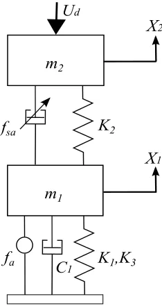
The example system under consideration in this paper is the multi-input multi-output (MIMO) two degree-of-freedom (2-DOF) nonlinear spring damper system shown in Fig. 1. The nonlinearity in the system is a weak cubic stiffness that comes in from the spring between mass m1 and the fixed support. As mentioned above, the weak non-linearity

is introduced in the system to represent the behavior associated with large deflections in a flexible structure. The system is subjected to a disturbance signal,Ud, that creates

unwanted vibrations of the two masses. The control objective is to minimize the motion of the masses using the combined action of the active and semi-active control devices.

An MR damper is used as a semi-active device because it is both reliable and widely available. The active device is a hydraulic actuator, and both this and the MR damper will be described in detail in Section 4. To simulate the situation in flexible structures that suffer from unwanted vibrations, the damping constant,C1, is chosen such that the

two degree-of-freedom system is under-damped. As a result the open-loop system has two lightly damped resonances.

The equation of motion for the two degree-of-freedom system is given by (1), where

X1 and X2 represent the displacement of mass m1 and m2 respectively, fa represents

the force of the active actuator,fsa represents the force of the semi-active actuator (MR

damper), m1, m2 represent the masses,K1, K2 are the linear spring stiffness,K3 is the

nonlinear spring stiffness, C1 is the damping coefficient and Ud is external disturbance

signal.

"

m1 0

0 m2

# "

¨

X1

¨

X2

#

+

"

C1 0

0 0

# "

˙

X1

˙

X2

#

+

"

K1+K2 −K2 −K2 K2

# " X1

X2

#

=

"

−K3

0

#

X₁3+

"

fa−fsa

fsa−Ud

#

(1)

The system can be represented in state space form as

˙

x1 =x2,

˙

x2 =

1

m1

fa−fsa−K1x1−C1x2−K2(x1−x3)−K3x31

,

˙

x3 =x4,

˙

x4 =

1

m2

fsa−K2(x3−x1)−Ud

,

(2)

where x1 and x2 are the position and velocity of mass m1 respectively, and x3 and x4

m₂

m1

fsa

fa

C1

Ud

K2

K1,K3

X1

X2

Figure 1. 2-DOF mass-spring-damper system, where fa represents the force of an

active actuator andfsa represents the force of a magneto-rheological damper. m1,m2 represent the masses,K1,K2are the liner spring stiffness,K3 is the nonlinear spring stiffness,C1 is the damping coefficient andUd is external disturbance signal

3. Immersion and Invariance & Sliding Mode Control

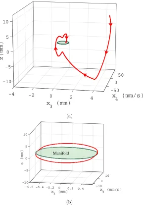
Fig. 2 shows a manifold, plotted from the data used in this paper, where x3 represents

the displacement andx4 represents the velocity andz represents the distance of

off-the-manifold dynamics from the off-the-manifold.

50

0

-50 -10

-5 0

-4 _-2

5

0 10

2 ₄

x

(mm/s)

z(mm)

x

3

(mm)

(a)

x

4 (mm/s) x

3 (mm)

z (mm)

10 0 -10

-5

-10 0

-0.6 -0.4 5

-0.2 0 10

0.2 0.4

Manifold

(b)

Figure 2. Manifold with off-the-manifold dynamics (a) transient phase , (b) steady state phase

In this paper we use the standard I & I approach [14]. The objective in the I & I theorem is to find a manifold M = {x ∈ _Rn_{|x = π(ξ), ξ ∈}

surface can be linear or nonlinear. The system trajectories are forced towards the sliding surface during the reaching mode and once on the sliding surface, the system trajectories are forced towards an asymptotically stable equilibrium point during the sliding mode. One of the differences mentioned in the literature between SMC and I & I is that in SMC the sliding surface needs to be reached by the trajectories whereas in I & I it is not necessary. The reason behind combining these two control techniques is that they share the same design approach and we can define a common target system for both the controllers. In the next two subsections the controller design is explained; the detailed derivation is given in Appendix B.

3.1. I&I Controller Design

The first step in the control design is to define a target/reference system. The target system should be realizable and should also consider the physical constraints of the actual system. In this example we set the control objective to control the vibrations in the mass m2. Therefore the target system is defined to reduce the flexible dynamics

to a single degree-of-freedom (SDOF) such that, in effect, the other degrees-of-freedom will behave as a rigid body motion. This means that the flexibility in the structure is reduced. It also aligns with the I & I methodology where the target system should be at least one degree less than the actual system.

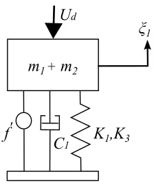
As a result the nonlinear SDOF system shown in Fig. 3 is defined as the target system. The aim of the controller design is to damp out the vibrations introduced by

Ud at m2. The dynamics of the target system are given as

m₁ + m₂

f'

C1 Ud

K₁,K₃ ξ₁

Figure 3. Target system, whereξ1 andξ2 represents the position and velocity of the mass(m1+m2), f

′

will be computed after defining the mapping functions,K1 is the liner spring stiffness,K3is the nonlinear spring stiffness,C1is the damping coefficient andUd is the external disturbance signal

˙

ξ1 =ξ2,

˙

ξ2 =

1 (m1+m2)

f′ −K1ξ1 −C1ξ2−K3ξ31−Ud

,

where ξ1 and ξ2 represent the position and velocity of the mass (m1+m2) respectively,

andf′ =W+u,urepresents the controller signal andWis the function that needs to be chosen in a way that the target system should have an asymptotically stable equilibrium at the origin. f′ is defined as

f′ =−C2(3K3ξ 2

1 +K1)ξ2

K2

+C1ξ2+u (4)

whereC2 is taken to be a linear approximation of the MR damping constant. The next

step is to design a controller for the target system. Any controller can be designed for the target system as long as it can achieve the desired performance for the defined mapping functions. In this paper a proportional plus integral (PI) controller is designed in the same way as in [40]. In the next step the asymptotic stability of the target system is derived using the Lyapunov theorem and the details are given in Appendix B. The mapping functions that need to be defined are given by

π(ξ) =



   

π1(ξ1, ξ2)

π2(ξ1, ξ2)

π3(ξ1, ξ2)

π4(ξ1, ξ2)



   

(5)

where π1(ξ1, ξ2), π2(ξ1, ξ2) need to be defined for off-the-manifold coordinates and

π3(ξ1, ξ2) = x3(π1, π2), π4(ξ1, ξ2) = x4(π1, π2). The mapping functions are derived for

off-the-manifold dynamics using the I & I theorem and the details are given in Appendix B. Finally the manifold is defined in-terms of off-the-manifold trajectories and then the control law is derived; the detailed derivation is in Appendix B.

3.2. SMC Controller Design

In the experimental system the semi-active device is a MR damper. The behavior of the damper has been thoroughly studied in previous literature; in the present work, the damper is modeled using the approach described in [41]. The controller for MR damper is designed using the SMC. A sliding surface is defined on which the system will be forced to slide. To make sure that the sliding surface has a asymptotic stable equilibrium point a Lyapunov candidate function is defined. To add robustness a discontinuous control is added to the equivalent control and finally to avoid the chattering phenomenon the Signum function is replaced with a tangent hyperbolic function. The detailed derivation of the SMC controller is given in Appendix B.

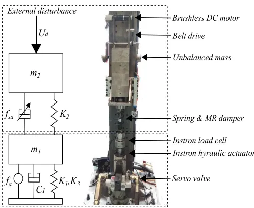
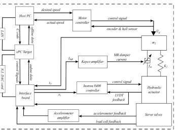
4. Experimental Setup

The experimental tests are performed as hardware-in-the-loop (HIL) tests. Fig. 4 shows the layout of the HIL experimental system. The physical part of the HIL test is the degree-of-freedom that includes mass m2, the MR damper and the linear spring.

The other degree-of-freedom that includes the mass m1, the active actuator, linear

m2

m1

fsa

fa

C1

Ud

K2

K1,K3

Brushless DC motor

Belt drive

Unbalanced mass

Spring & MR damper

Instron load cell Instron hyraulic actuator

Servo valve External disturbance

Figure 4. Hardware-in-the-loop (HIL) test set-up, wherefa represents the force of the

active actuator and fsa represents the force of the magneto-rheological damper. m1, m2 represent the masses, K1, K2 are the liner spring stiffness, K3 is the nonlinear spring stiffness, andC1 is the damping coefficient

simulated numerically and applied to the physical system via a force applied by the Instron hydraulic actuator.

The displacement of mass m1 from Simulink goes into the Instron 8400 controller

via a National Instruments data acquisition card as shown in Fig. 5. The control signal from the Instron 8400 controller goes to the Instron hydraulic actuator via servo valves and the LVDT gives the feedback displacement signal.

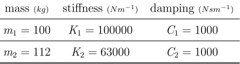
Table 1 shows the parameters of the 2-DOF system and Table 2 shows the gains designed for PI, I&I and SMC controllers. Fig. 6 shows the block diagram implementation of the hybrid control. Here, fi&i is the control signal of the I & I

controller that goes into the non-physical DOF. The displacement x1 of mass m1 then

goes into the Instron controller. Finally the control signalfafrom the Instron controller

goes into the hydraulic actuator via servo valves. The simulated models for the Instron controller, servo valves and hydraulic actuator are provided by the manufacturer.

The MR damper is used as semi-active device and fid is the control signal of the

SMC. The input of the MR damper is a current signal, so a controller is designed to convert the SMC control signal to a current signal. As a result, IM R is the current

control signal that goes into the MR damper as shown in Fig. 6.

Motor controller

Instro

controller

A ometer

I

board

x arget

H o

N

C c

ar

d

L

Figure 5. Experimental setup, where the Simulink file is transferred from host PC to XPC target through LAN. Data is sent in and out in real time from XPC target through a N.I. DAC card,IM Ris the control current signal that first goes to the Kepco

amplifier and then to the MR damper. x1 is the displacement of mass m1 which goes to the Instron 8400 controller and then to the Instron hydraulic actuator. The displacement feedback signal from the LVDT is sent to the Instron 8400 controller and the XPC target. The accelerometer feedback signal goes to the XPC target through an amplifier and load cell that gives the combined force of spring and damper that is sent to the XPC target

5. Simulation & Experimental Results

For all the simulation and experimental results, in the first 5 seconds the system is vibrating in open loop after which the controller is switched on. Fig. 9 shows the displacement of mass m2 being controlled to follow the reference signal in which

a single mass, m1 + m2, is assumed. It can be seen that the simulated system is

Simulated Immersion & Invariance

control

x1 f_id I

MR controller

IMR id

arget

system

i&i

Sliding mode control

1

, 2

, 3

, 4

]

Figure 6. Block diagram implementation of hybrid active & semi-active control, where x1 and x2 are the position and velocity of mass m1 respectively, x3 and x4 are the position and velocity of massm2respectively,fi&iis the I & I control signal,fais force

of the active actuator, fsa is force of the MR damper,IM R is output of the controller

that converts the SMC control signalfid to the current signal for MR damper

Immersion & Invariance

contr!!" #

Mapping and

M"$ %&!' ()

controller +

_ R*&* -ence

signal .i&i

z /

z 0

u e

x5

67 8 6 /

9 6 0

9 6 5

9 6 :

;

Figure 7. Block diagram implementation of I & I controller, wherex1 andx2 are the position and velocity of massm1respectively,x3andx4 are the position and velocity of massm2respectively,fi&i is the I & I control signal,z1andz2 are the error dynamics in I & I controller, uis output of the PI controller, e is error between reference and desired signal

Table 1. System parameters

mass (kg) stiffness (N m−1₎ damping _{(N sm}−1₎

Sliding mode contr<== >?

@id Sliding

sB CD>EF

GF DF Cence signal

JK controller O

P

Target system S

u e

Q

SUV S Q

W S X

W S Y

WS Z

[

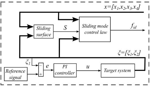
UV Q

W X

[

Figure 8. Block diagram implementation of SMC controller, wherex1andx2are the position and velocity of mass m1 respectively, x3 andx4 are the position and velocity of massm2 respectively, uis output of the PI controller, e is error between reference and desired signal,fid is the output of the SMC controller,S is the sliding surface,ξ1 andξ2 represent the position and velocity of the mass (m1+m2) respectively

Table 2. Controller gains

PI controller I&I controller SMC controller

Kp = 5.43 k1 = 1000 K = 1

Kv = 7420 k2 = 15.00 λ1 = 1

Ki = 67722 λ2 = 1

4 5 6 7 8

time (sec)

-4 -2 0 2 4

displacement (mm)

experiment simulation reference system

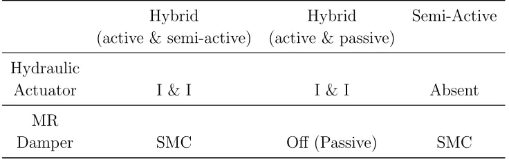
Table 3. Simplified controller architecture used for comparison

Hybrid Hybrid Semi-Active

(active & semi-active) (active & passive)

Hydraulic

Actuator I & I I & I Absent

MR

Damper SMC Off (Passive) SMC

6. Comparison With Other Controllers

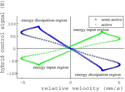
To illustrate the effectiveness of proposed hybrid active & semi-active controller, it is compared to two straightforward scenarios with reference to Table 3. The hybrid active & passive controller involves using the MR damper as a purely passive device. For the semi-active controller, the hydraulic actuator is completely absent from the system. Fig. 10 shows the active and semi-active control signal in the hybrid active & semi-active controller. Here, the MR damper can only work in the dissipative region and when energy is required to be injected into the system then the active actuator is assisting the semi-active actuator.

One of the main problems with the semi-active controller is ”clipping” [42], which occurs when the semi-active device is unable to inject energy into the system. Fig. 11a and 11b shows the semi-active control signals with respect to the relative velocity and time in hybrid active & semi-active and semi-active controllers respectively. The clipping is reduced to a larger extent in the hybrid active & semi-active controller as compared to the semi-active controller because as the controller switches off in the hybrid active & semi-active controller, the active actuator injects the desired energy and the semi-active actuator returns back to the dissipative region.

Fig. 12a shows the experimental displacement of mass m2 with the semi-active

controller. After 5 seconds the controller is turned on and the actual system (2) cannot achieve the target system (3). Fig. 12b also shows the displacement of mass m2 with a

hybrid active & passive controller, its performance is better than semi-active controller, but still it cannot achieve the target system. However, in all cases the proposed hybrid active & semi-active controller is able to achieve the target system as shown in Fig. 9. A fully active system will behave exactly in the same way as the target system, so that is why all the comparisons are made on the basis of how close the performance is to the target system.

-5 0 5 relative velocity (mm/s) -100

-50 0 50 100

hybrid control signal (N)

semi-active active

energy dissipation region energy dissipation region

energy input region

energy input region

Figure 10. Active & semi-active control signals in hybrid active & semi-active controller

the active actuator can inject energy to reach the target system. However the main focus in this paper is using the active actuator to assist a semi-active device. If the amplitude of the disturbance is increased from 70 N to 1000 N then the difference in the performance of the controller can be seen more clearly in Fig. 13c. Using a disturbance signal with an amplitude of 1000 N is an extreme test and too severe to be implemented practically. Consequently, only simulation results are shown for this scenario. The main reason to perform this test in simulation is to show that at higher amplitude excitations, the difference in the performance of the controllers is more obvious.

Fig. 14 and 15 shows the manifold with off-the-manifold dynamics and sliding surface with error dynamics respectively in three different case. In the first case both the controllers are in the off state. In the second case the semi-active controller is turned on and the distance between the manifold and off-the-manifold dynamics is decreased. In the third case the hybrid controller is turned on and off-the manifold dynamics comes very close to the manifold. Same pattern is followed by the error dynamics in Fig. 15.

-20 -10 0 10 20

relative velocity (mm/s)

-150 -100 -50 0 50 100 150

control signal (N)

hybrid controller semi-active controller

(a)

7.5 8 8.5

time (sec)

-150 -100 -50 0 50 100 150

control signal (N)

semi-active controller hybrid controller

(b)

3 4 5 6 7 8 time (sec) -4 -2 0 2 4 displacement (mm) (a)

3 4 5 6 7 8

time (sec) -4 -2 0 2 4 displacement (mm) (b)

Figure 12. Displacement of mass m2 controlled to follow the reference system (experiment), (a) with a semi-active controller, (b) with hybrid active & passive controller

-4 -2 0 2 4 6

e (mm) -60 -40 -20 0 20 40 60 ˙ e (m m /s ) passive semi-active hybrid (1) hybrid (2) (1) active+passive (2) active+semi-active (a)

-4 -3 -2 -1 0 1 2 3 4 5 6

e (mm) -100 -80 -60 -40 -20 0 20 40 60 80 100 ˙ e (m m / s) passive semi-active hybrid (1) hybrid (2) (1) active+passive (2) active+semi-active (b)

-100 -50 0 50 100 150 e (mm) -1500 -1000 -500 0 500 1000 1500 ˙ e (m m /s ) passive semi-active hybrid (1) hybrid (2) (1) active+passive (2) active+semi-active (c)

Figure 13. (a) error dynamics withUd=70 N (simulation), (b) error dynamics with

x

3 (mm)

z (mm)

x

4 (mm/s) 10

0 -15

-10 -5

-10 0

-0.6 5

-0.4 10

-0.2 0

15

0.2 0.4

Manifold

15.41 mm

(a)

x

4 (mm/s) x

3 (mm)

z (mm)

10 0 -15

-10 -5

-10 0

-0.6 5

-0.4 10

-0.2 15

0 0.2 0.4

Manifold

8.06 mm

(b)

x 3 (mm)

z (mm)

x

4 (mm/s) 10 0 -15

-10 -5

-10 0

-0.6 5

-0.4 10

-0.2 0 15

0.2 0.4

Manifold

1.67 mm

(c)

Figure 14. Manifold with off-the-manifold dynamics (a) in open loop , (b) with semi-active controller, (c) with hybrid controller

One of the advantages of an MR damper is its low energy consumption, which comes with the cost of passivity constraint. Fig. 16a shows the energy consumption of the MR damper in passive, semi-active and hybrid control regions. The energy consumption of the MR damper is taken to be,

EC =R

Z t

0

i2dt (6)

where i is the input current to the MR damper, R is the resistance and EC is

e

(m

m

)

ξ2(mm/s)

ξ1(mm) 0.5

0 -5

10 ₅ 0 0

-0.5 -5 _-10 5

Sliding surface

4.67 mm

(a)

ξ1(mm)

e

(m

m

)

ξ2(mm/s)

0.5

0 -5

10 ₅ 0 0

-0.5 -5 _-10 5

2.45 mm

Sliding surface

(b)

ξ1(mm)

ξ2(mm/s)

e

(m

m

)

0.5

0 -5

10

5 ₀

0

-0.5 -5 _-10 5

Sliding surface

(c)

Figure 15. Sliding surface with error dynamics (a) in open loop , (b) with semi-active controller, (c) with hybrid controller

damper which is given as,

ED =

Z t

0

fsaVrdt (7)

where fsa is the MR damper output force, Vr is relative velocity across the MR

damper and ED is MR damper dissipative energy. The dissipative energy keeps on

decreasing as we move from passive to semi-active and finally to the hybrid region. On the other hand, the performance keeps on showing significant improvement. In Fig. 16b, only the MR damper energy consumption is compared in the passive, semi-active and hybrid region. The overall energy consumption comparison of the hybrid controller that includes both the active actuator and the semi-active device cannot be made with the passive or semi-active cases, as there is no active actuator involved in the later two cases.

0 2 4 6 8 10 12 14 time (sec)

0 0.5

1 1.5

2

E C

(J)

Semi-active region Passive

region Hybrid _region

(a)

0 2 4 6 8 10 12 14

time (sec) 0

5 10 15 20 25 30

E D

(J)

Semi-active region

Hybrid region Passive

region

(b)

Figure 16. (a) MR damper energy consumption (experiment), (b) MR damper energy dissipation (experiment)

0 1 2 3 4 5 6 7

frequency (Hz)

0 0.5

1 1.5

x 3

(mm)

Passive Semi-active Hybrid

(a)

0 1 2 3 4 5 6 7

frequency (Hz)

0 0.5

1 1.5

x 3

(mm)

Passive Semi-active Hybrid

(b)

Figure 17. Frequency response, (a) simulation, (b) experimental

7. Discussion

For a quantitative analysis of the three controllers compared in Section 6, a performance index is defined as an absolute value of the radius of phase plane shown in Fig. 13. From this it can be seen when the proposed hybrid active & semi-active controller is turned on, the error is reduced by 88%. In comparison, the other two controller i.e. hybrid active & passive and semi-active, the error is reduced by 73% and 41% respectively. In Fig. 13, the amplitude of the disturbance signal has been increased from 70 N to 1000 N. The proposed hybrid active & semi-active controller has reduced the error by 92% and the other two controllers have reduced the error by 68%. The reference used in this quantitative comparison are the simulation results. Therefore the performance of proposed hybrid active & semi-active controller is better than the other two controllers in both the cases of low and high amplitude disturbance signals. In the case of high amplitude disturbance signal, the performance index of the proposed hybrid active & semi-active controller has been further increased by 4%.

This idea is general, and is not restricted to either the controller methodologies, or the example presented in this paper. The same results might be achieved by combining different control techniques, however this is beyond the scope of the current proof-of-concept study. The experimental setup shown in Fig. 4 is chosen because it represents a relatively simple test bed system that can be readily compared to simulation results. HIL testing is used because there is a freedom to change the system parameters in the simulated part of the model which in this study included the non-linearity.

8. Conclusion

A new robust hybrid active & semi-active control technique has been introduced in which an active actuator is assisting the semi-active device to achieve the performance close to a fully active system. The switching time of the semi-active controller has been reduced to a large extent by the hybrid active & semi-active controller because the active actuator injects the desired energy as the semi-active controller switches off, following which the semi-active device returns back to the dissipative region. The proposed control technique has been compared with semi-active and hybrid active & passive controllers. Based on the performance index defined in Section 7, the proposed controller performance is better than the other two controllers. The idea has been implemented on a 2-DOF mass-spring-damper system example that also includes a cubic stiffness non-linearity. The results from both simulations, and HIL experiments showed good results in terms of achieving the control objectives.

Acknowledgment

References

[1] Fujita T; IEEE. Application of hybrid mass damper with convertible active and passive modes using hydraulic actuator to high-rise building. American Control Conference. 1994;1:1067–1072. [2] Fujinami T, Saito Y, Morishita M, Koike Y, Tanida K. A hybrid mass damper system controlled by H-infinity control theory for reducing bending-torsion vibration of an actual building. Earthquake engineering & structural dynamics. 2001;30(11):1639–1653.

[3] Kim H, Adeli H. Hybrid Control of Smart Structures Using a Novel Wavelet-Based Algorithm. Computer-Aided Civil and Infrastructure Engineering. 2005;20(1):7–22.

[4] Rao M, Ram T, Purushottam A. Analysis of passive and semi active controlled suspension systems for ride comfort in an omnibus passing over a speed bump. International Journal of Research & Reviews in Applied Sciences. 2010;5(1).

[5] d’Azzo JJ, Houpis CD. Linear control system analysis and design: conventional and modern. McGraw-Hill Higher Education; 1995.

[6] Kaczorek T. Linear Control Systems: analysis of multivariable systems. John Wiley & Sons, Inc.; 1992.

[7] Sastry S. Nonlinear systems: analysis, stability, and control. Springer New York; 1999.

[8] Zhou HM, Zheng XJ, Zhou YH. Active vibration control of nonlinear giant magnetostrictive actuators. Smart Materials and Structures. 2006;15(3):792.

[9] Fazelzadeh SA, Jafari SM. Active control law design for flutter suppression and gust alleviation of a panel with piezoelectric actuators. Smart Materials and Structures. 2008;17(3):035013. [10] Diaz I, Reynolds P. Robust saturated control of human-induced floor vibrations via a proof-mass

actuator. Smart Materials and Structures. 2009;18(12):125024.

[11] Astolfi A, Ortega R. Immersion and invariance: a new tool for stabilization and adaptive control of nonlinear systems. IEEE Transaction on Automatic Control. 2003;48(4):590–606.

[12] Karagiannis D, Astolfi A, Ortega R. Nonlinear stabilization via system immersion and manifold invariance: survey and new results. MMS. 2005;3(4):801–817.

[13] Astolfi A, Karagiannis D, Ortega R. Towards applied nonlinear adaptive control. Annu Rev Control. 2008;32(2):136–148.

[14] Astolfi A, Karagiannis D. Nonlinear and adaptive control with applications. Springer Science & Business Media; 2007.

[15] Zhao B, Xian B, Zhang Y, Zhang X. Nonlinear Robust Adaptive Tracking Control of a Quadrotor UAV Via Immersion and Invariance Methodology. IEEE Transactions on Industrial Electronics. 2015 May;62(5):2891–2902.

[16] Santhanapipatkul P, Khovidhungij W. Nonlinear controller design for active suspension systems using the immersion and invariance method. World Congress. 2005;16(1):1934–1934.

[17] Wimbock T, Ott C, Hirzinger G; IEEE. Immersion and invariance control for an antagonistic joint with nonlinear mechanical stiffness. Proceedings of 49th IEEE Conference on Decision and Control. 2010;p. 1128–1135.

[18] Dib W, Kenn´e G, Lamnabhi-Lagarrigue F. An application of Immersion and Invariance to transient stability and voltage regulation of power systems with unknown mechanical power. Proceedings of 48th IEEE CDC. 2009;p. 7837–7842.

[19] Khan IU, Dhaouadi R; IEEE. Vibration suppression in elastic drive systems using the immersion and invariance methodology. 3rd International Conference on Electric Power and Energy Conversion Systems. 2013;p. 1–6.

[20] Emelyanov S. Variable structure control systems. Moscow, Nouka. 1967;.

[21] VADIM IU. Survey paper variable structure systems with sliding modes. IEEE Transactions on Automatic control. 1977;22(2).

[22] Utkin V. Variable structure systems- Present and future. Automation and Remote Control. 1984;44(9):1105–1120.

Electronics. 1993;40(1):2–22.

[24] Young KD, Utkin VI, Ozguner U. A control engineer’s guide to sliding mode control. IEEE Transactions on Control Systems Technology. 1999;7(3):328–342.

[25] Yu X, Kaynak O. Sliding-Mode Control With Soft Computing: A Survey. IEEE Transactions on Industrial Electronics. 2009 Sept;56(9):3275–3285.

[26] Song G, Gu H. Active vibration suppression of a smart flexible beam using a sliding mode based controller. Journal of Vibration and Control. 2007;13(8):1095–1107.

[27] Piltan F, Boroomand B, Jahed A, Rezaie H. Methodology of Mathematical Error-Based Tuning Sliding Mode Controller. International Journal of Engineering. 2012;6(2):96–112.

[28] Nguyen VQ, Choi SB. A robust vibration control for a multi-active mount system subjected to broadband excitation. Smart Materials and Structures. 2011;20(5):055002.

[29] Lu KC, Loh CH, Yang JN, Lin PY. Decentralized sliding mode control of a building using MR dampers. Smart Materials and Structures. 2008;17(5):055006.

[30] Assadsangabi B, Eghtesad M, Daneshmand F, Vahdati N. Hybrid sliding mode control of semi-active suspension systems. Smart Materials and Structures. 2009;18(12):125027.

[31] Yao Jl, Shi Wk, Zheng Jq, Zhou Hp. Development of a sliding mode controller for semi-active vehicle suspensions. Journal of Vibration and Control. 2013;19(8):1152–1160.

[32] Assadsangabi B, Eghtesad M, Daneshmand F, Vahdati N. Hybrid sliding mode control of semi-active suspension systems. Smart Materials and Structures. 2009;18(12):125027.

[33] Bartolini G, Pisano A, Punta E, Usai E. A survey of applications of second-order sliding mode control to mechanical systems. International Journal of Control. 2003;76(9-10):875–892. [34] Levant A. Higher-order sliding modes, differentiation and output-feedback control. International

journal of Control. 2003;76(9-10):924–941.

[35] Bartolini G, Ferrara A, Usani E. Chattering avoidance by second-order sliding mode control. IEEE Transactions on Automatic control. 1998;43(2):241–246.

[36] Gu H, Song G, Malki H. Chattering-free fuzzy adaptive robust sliding-mode vibration control of a smart flexible beam. Smart Materials and Structures. 2008;17(3):035007.

[37] Soong T, Spencer Jr B. Supplemental energy dissipation: state-of-the-art and state-of-the-practice. Engineering Structures. 2002;24(3):243–259.

[38] Spencer Jr B, Nagarajaiah S. State of the art of structural control. Journal of structural engineering. 2003;129(7):845–856.

[39] Fisco N, Adeli H. Smart structures: part-I active and semi-active control. Scientia Iranica. 2011;18(3):275–284.

[40] Khan I, Dhaouadi R. Robust Control of Elastic Drives through Immersion and Invariance. IEEE Transactions on Industrial Electronics. 2015;62(3):1572–1580.

[41] Sims ND, Holmes N, Stanway R. A unified modelling and model updating procedure for electrorheological and magnetorheological vibration dampers. Smart materials and structures. 2004;13(1):100.

Appendix A. I & I Conditions

Consider a nonlinear system

˙

x=f(x) +g(x)u (A.1)

wherex∈Rnis the system state,u∈Rmis the input signal,f(x) andg(x) are nonlinear functions of x and an over-dot represents the differentiation with respect to time. The equilibrium point to be stabilized is denotedx⋆ _∈

Rn. The following properties should hold.

(H1) The system ˙

ξ=α(ξ) (A.2)

with transformed state vector ξ ∈ Rp _{has an asymptotically stable equilibrium at}

ξ⋆ ∈Rp_{, and}

x⋆ ∈π(ξ⋆).

where α:Rp →Rp and π :Rp →Rn are smooth mapping functions with p < n. (H2) For all ξ ∈Rp, substituting a smooth mapping x=π(ξ) in (A.1) leads to

f(π(ξ)) +g(π(ξ))c(π(ξ)) = ∂π

∂ξα(ξ). (A.3)

where c:Rp _→Rm _{is the control signal that renders the manifold invariant.}

(H3) The set identity holds

{x∈Rn|φ(x) = 0}={x∈Rn|x=π(ξ), ξ ∈Rp}. (A.4)

where φ : Rn → Rn−_p

represents the manifold. From (A.4), the manifold φ(x) = 0, when x =π(ξ), hence φ =x−π(ξ) and z = x−π(ξ), where z represents the distance between off-the-manifold coordinates and the manifold.

(H4) All trajectories of the system

˙

z = ∂φ

∂x[f(x) +g(x)ψ(x, z)], (A.5)

˙

x=f(x) +g(x)ψ(x, z), (A.6)

are bounded and satisfy

lim

t→∞

z(t) = 0. (A.7)

where ψ : _Rn×(_n−_p)

→ _Rm _{is the equivalent control signal and right hand side of (A.5)}

is ˙φ. Then x∗

is an asymptotically stable equilibrium of the closed loop system

˙

x=f(x) +g(x)ψ(x, φ(x)). (A.8)

Once the close loop system (A.8), trajectories converges to the manifold andz = 0 then

Appendix B. Controller Design

Appendix B.1. I&I Controller Design

The implementation of the PI controller in the target system is given by

u=Ki

Z

evdt+Kvev

where

ev =Kpep−ξ2

and the PI control signal is given as

u=Kaep+Kb

Z

epdt−Kcξ2−Kdξ1 (B.1)

where, Ki, Kv & Kp are control gains, ev is the velocity error, ep is the position error,

and Ka =KvKp, Kb =KiKp,Kc =Kv, Kd=Ki. To check the asymptotic stability of

the target system, the target system dynamics are compared with a single mass system dynamics (B.2). From the Lagrangian formulation the dynamics of a single mass are

˙

ξ₁ =ξ₂

˙

ξ₂ =−E′ −ξ₂R (B.2)

where E is the potential energy function and R is the damping function and a dash represents differentiation with respect to the state vector.

Comparing (3) and (B.2) gives

E′ = K1ξ1+K3ξ

3 1

(m1+m2)

(B.3)

R= C2(3K3ξ

2

1 +K1)

K2(m1+m2)

(B.4)

and

E = K1ξ

2 1

2(m1+m2)

+ K3ξ

4 1

4(m1+m2)

. (B.5)

A Lyapunov function is defined as a generalized energy function

Vi&i =

1 2ξ2

2_{+E. (B.6)}

The target system dynamics will have an asymptotically stable equilibrium at the origin if the following conditions are satisfied by the Lyapunov function defined in (B.6)

V(0,0) = 0 (B.7a)

V (ξ₁, ξ₂)>0, in D− {0}. D→Rp (B.7b)

˙

whereV (ξ₁, ξ₂) is the energy function, andDis the subset of_Rp _{in which the Lyapunov}

function is defined. As a result

˙

Vi&i(ξ1, ξ2) = ξ2ξ˙2+E

′ ξ₂,

˙

Vi&i(ξ1, ξ2) = ξ2

˙

ξ₂+E′,

From (B.2) ˙

Vi&i(ξ1, ξ2) = −Rξ22. (B.8)

The first two conditions (B.7a) and (B.7b) are satisfied by the Lyapunov function defined in (B.6). The third condition (B.7c) where ˙Vi&i(ξ1, ξ2) should be negative definite, is

satisfied whenRis positive. As can be seen from (B.4),R is always positive. Therefore, the selected target system has an asymptotically stable equilibrium at the origin.

It is difficult to solve the partial differential equation (A.3). Since the target system dynamics (3) resembles the part of actual system dynamics (2), so the solution of (A.3) can be obtained by setting π3(ξ1, ξ2) =ξ1. As ˙x1 =x2, so we can write π4(ξ1, ξ2) =ξ2.

Therefore, the mapping functions π1(ξ1, ξ2), π2(ξ1, ξ2) are derived from

˙

ξ₂ = ˙π4. (B.9)

and

1

m1+m2

f′ −K1ξ1−C1ξ2−K3ξ13

= 1

m2

−C2(ξ2−π2)−K2(ξ1−π1)

(B.10)

The selection of the mapping functions is a non trivial task and it is possible for more then one mapping function to exist. However, they should always satisfy (B.10) and by using these mapping functions, the target system should have an asymptotically stable equilibrium at the origin. Therefore the mapping functions selected are

π1 =−α1

m2K3ξ31

K2(m1+m2)

− m2K1ξ1

K2(m1+m2)

+ξ1+α2ep +α3

Z

epdt+α4ξ2+α5ξ1,

(B.11)

π2 =

−α1

3m2K3ξ12

K2(m1+m2)

− m2K1

K2(m1+m2)

+ 1ξ2−α2ξ2+α3ep+α4ξ˙2 +α5ξ2.

Substituting π1, π2 and f

′

in (B.10) gives

1

m1+m2

"

− C2(3K3ξ 2

1 +K1)ξ2

K2

+C1ξ2+Kaep+Kb

Z

epdt−Kcξ2−Kdξ1−K1ξ1

−C1ξ2−K3ξ31

#

= 1

m2

"

−C2 ξ2−

−α1

3m2K3ξ12

K2(m1+m2)

− m2K1

K2(m1+m2)

+ 1 ξ2

−α2ξ2+α3ep+α4ξ˙2+α5ξ2

!

−K2 ξ1−

−α1

m2K3ξ13

K2(m1+m2)

− m2K1ξ1

K2(m1+m2)

+ξ1 +α2ep+α3

Z

epdt+α4ξ2+α5ξ1

!#

(B.13)

Using (B.13), we now compare coefficients to find out the five unknowns α1, α2,α3,α4,

α5.

                   

0 0 0 C2(Kd−K1)

m2(m1+m2)

K2

m2

0 K2

m2

C2

m2

KaC2

m2(m1+m2)

0

0 0 K2

m2

KbC2

m2(m1+m2)

0

1 0 0 C2

m2

0

0 C2

m2

0 − C2

m2(m1+m2)

−K1C2−KcK2

K2

− K2

m2

−C2

m2                                        α1 α2 α3 α4 α5                    =                    Kd

m1+m2

Ka

m1+m2

Kb

m1+m2

1

Kc

m1+m2

                   (B.14)

The error between the off-the-manifold dynamics and the mapping functions is defined as

φ(x) =x₁−π1 (B.15)

and the manifold is defined as

where ˙φ(x) = x2−π2. The gainsk1 and k2 are chosen in such a way that (s2+k2s+k1)

is Hurwitz.

The last step in the I&I methodology is to compute the control law, which is done using

¨

φ= ˙x2−π˙2 (B.17)

and

¨

φ = 1

m1

fa−fsa−K1x1−C1x2−K2(x1−x3)−K3x31

− ∂π2

∂x3

˙

x3−

∂π2

∂x4

˙

x4. (B.18)

The control signal fa is given by

fa=

"

−k1φ−k2φ˙+

∂π2

∂x3

˙

x3+

∂π2

∂x4

˙

x4

#

m1 +K1x1+C1x2+K2(x1−x3)+

C2(x2−x4) +K3x31 (B.19)

where

∂π2

∂x3

=−6α1K3m2x3x4

K2(m1 +m2)

−α3−

α4K2

m2

, (B.20)

∂π2

∂x4

= (−3α1K3x

2

3−K1)m2

K2(m1+m2)

+ 1−α2−

α4C2

m2

+α5 (B.21)

Appendix B.2. SMC Controller Design

The sliding mode control is designed to control the semi-active device. The error dynamics are defined as

e=x3−ξ1. (B.22)

The sliding surface is defined in terms of the error dynamics as

S=λ1e+λ2e˙ (B.23)

where λ1, λ2, are the design parameters, which will determine how fast the error

dynamics will go to zero and ˙e=x4−ξ2. In the next step the control signal is derived

using (B.23).

fsa =fn−

m2

λ2

Ksmcsgn(S)

(B.24)

where Ksmc is strictly positive and a design parameter and fn is given as

fn =

m2

λ2

−λ1(x4−ξ2)

!

+m2ξ˙2+K2(x3−x1) +Ud. (B.25)

SMC control signal has two parts. One part represents the normalized controlfnand the

equilibrium at the origin towards which the system will slide, a Lyapunov function is defined as

Vsmc=

1 2S

2_{. (B.26)}

The sliding surface will have an asymptotically stable equilibrium if (B.26) satisfies the conditions in (B.7). The first two conditions (B.7a) and (B.7b) are satisfied by the Lyapunov function defined in (B.26), for the third condition (B.7c) to be satisfied, ˙Vsmc

needs to be analyzed, where ˙

Vsmc=SS˙

and

SS <˙ 0

To make sure that the system will reach the sliding surface in finite time, a more strict condition is imposed on SS˙

SS˙ ≤ −η|S| (B.27)

where η is strictly positive. Then

SS˙ ≤ −ηSsgn(S)

and

˙

S≤ −ηsgn(S)

such that

Ksmc≥η. (B.28)

For the third condition to be satisfied for an asymptotically stable equilibrium, Ksmc

should be greater than η. The MR damper can only dissipate energy from the system. The controller will be switched-on, when the relative velocityVr across the MR damper

and the control signal fsa have opposite signs and will be switched-off otherwise. This

condition is imposed on fsa in (B.29) and is called the passivity constraint:

fsa =





 fn−

m2

λ2

Ksmcsgn(S)

fsaVr <0

0 fsaVr >0

(B.29)

where Vr =x4−x2.

To avoid chattering, we have used the approximation that the Signum function can be replaced with the tangent hyperbolic function

sgn(x)≈tanh(kx) (B.30)