An input output model of the Tasmanian economy

AN INPUT—OUTPUT MODEL

OF THE TASMANIAN ECONOMY

George C. Edwards

Submitted in fulfilment of the requirements for the degree of

Master of Economics

UNIVERSITY OF TASMANIA ROBAICE

The material generated by this research has not been

accepted for the award of any other degree or diploma in

any university. To the best of my knowledge and belief,

the thesis contains no copy or paraphrase of material

previously published or written by another person except

ACKNOWLEDGMENTS

This study would not have been possible without the co-operation

and assistance rendered by the Deputy Commonwealth Statistician and

members of staff of the Hobart office of the Australian Bureau of

Statistics. Grateful acknowledgment is also made to officers of the

Industries Assistance Commission and the Biometrics Section of the

Tasmanian Department of Agriculture for assistance with matrix

- TABLE OF CONTENTS

Page

LIST OF FIGURES

LIST OF TABLES vi

ABSTRACT vii

CHAPTER. 1 INTRODUCTION

1.1 Objectives and Origins

CHAPTER 2 INPUT-OUTPUT ECONOMICS

2.1 The Input-Output System 3

2.2 The Assumptions 10

2.3 Variants to the Open Static Model 14

CHAPTER 3 ECONOMIC ANALYSIS WITH INPUT-OUTPUT MODELS

3.1 Input-Output and Economic Development 21

3.2 Qualitative Analysis 22

3.3 Quantitative Analysis 24

CHAPTER 4 REGIONAL INPUT-OUTPUT MODELS

4.1 The Development of Regional Models 29

4.2 Australian Input-Output Studies 33

4.3 The Need for a Tasmanian Regional Study 34

CHAPTER 5 PROCEDURE AND DATA SOURCES

5.1 The Integrated Censuses 39

5.2 The Selection of Industries 40

5.3 Construction Procedure for the

Transactions Table 43

5.4 The Treatment of Conceptual Problems 50

CHAPTER 6 RESULTS

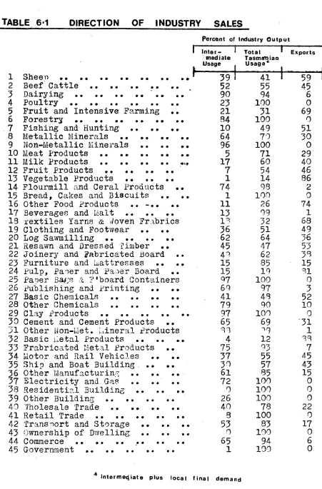
6.1 The Transactions Table 56

6.2 National Accounting 61

6.3 Technical Coefficients 63 6.4 Interdependence Coefficients and

Output Multipliers 65

6.5 Income Multipliers 67

6.6 Model Closure 73

.Page

CHAPTER 7 CONCLUSIJNS

7.1 The Results in Perspective 84

7.2 The Need for Further Research 85

7.3 Some Further Applications of the Model 87

APPENDIX 1 Transactions Table: Tasmania 1968-69

APPENDIX 2 Table of Input Coefficients

APPENDIX 3 Table of Interdependence Coefficients

BIBLIOGRAPHY 91

LIST OF FIGURES

Page

Figure 2.1 Quadrants of the Transactions Table 5

2.2 Factor - Factor Diagram 13

2.3 Closing the Input-Output Model 16

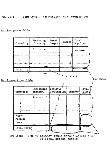
5.1 _ Flow Diagram 44

5.2 Compilation Arrangements for Transactions 46

6.1 Relative Size of Industries: Input-Output

Table 57

6.2 Comparative Size: Industry Sectors

Tasmania and Australia 60

6.3 Direct, Indirect and Induced Income

Change 69

vi

LIST OF TABLES

Page

Table 4.1 _{Average Income and Wages . - Australia 0 35}

5.1 Industry Classification in Terms of ASIC 42

5.2 Make Matrix of the Manufacturing Sector ₄₇

6.1 Direction of Industry Sales ₅₈

6.2 Tasmanian and Australian Production

Accounts 1968-69 62

6.3 Source of Industry Inputs ₆₄

6.4 Output Multipliers in Ranked Order ₆₆

6.5 Output and Income Multipliers 68

6.6 Type I Income Multipliers in Ranked Order 71

6.7 Type II Income Multipliers in Ranked Order 72

6.8 Effects of Different Model Closure Methods 76

6.9 Workforce and Employment Multipliers 78

6.10 Employment Multipliers in Ranked Order 80

6.11 Direct, Indirect and Induced Employment 82

vii

ABSTRACT

Input-output economics is an internationally accepted method of

economic planning and decision making but the construction of

input-output models within Australia has not been extensive even though a

national transactions table was cOnstructed early in the era of

input-output. Over the last decade the situation has been changing

with national tables, now constructed on a regular basis and

regional studies proliferating. The major obstacle to the

preparation of sub-national input-output tables is the paucity of

commodity and trade data so that for most regional studies the

emphasis has been on surveys. For two States, Western Australia and

Tasmania, both commodity and trade data are tabulated by the

Australian Bureau of Statistics thus providing the basis for the

construction of input-output models principally from secondary data.

An interindustry study for W.A. appeared in 1967. The aim of this

study is to produce a Tasmanian transactions table together with the

associated tables of coefficients and to quantify the structural

economic inter-relationships by determining the output, income and

employment multipliers of Tasmanian industries.

In Chapter 2 the input-output system and the assumptions are

presented together with the mathematical relationships. The closed

model and the dynamic input-output system incorporating capital

coefficients, both extensions to the basic open static model, are

also described. The forms of input-output analysis are outlined in

viii

Input-output analysis has assumed a dominant position in

regional research and in Chapter 4 the development of regional

models is outlined through a review of the pertinent sections of

the literature. The Australian involvement is also traced.

Regional studies are frequently motivated by regional problems and

the need to provide planning techniques to lift regional prosperity.

It is shown that the Tasmanian economy provides such an instance.

Chapter 5 is concerned with construction procedure and

conceptual problems encountered in compilation. The sources of

data are indicated and the selection of processing industries, final

demand and processing sectors discussed. Producer prices are

selected and competitive imports allocated directly.

The results are presented in Chapter 6. The main

character-istics of the 45 industry transactIms table, the table of input

coefficients and the table of interdependence coefficients, are

described. The components (direct, indirect and induced) of total

income change per dollar change in final demand are generated

together with type I and type II income multipliers. The problems

encountered in closing the model are discussed and the range of

results produced by different closure methods outlined. The direct,

indirect and induced employment effects are presented along with

type I and type II employment multipliers.

The final chapter sets the achieved objectives in perspective

with other Australian studies. The deficiencies of the model are

discussed along with suggestions for further research related to

CHAPTER 1

INTRODUCTION

1.1 Objectives and Origins

The objectives of this study were:

(1) to construct an input-output transactions table

for the State of Tasmania and determine the

associated tables of coefficients

(2) to quantify the structural inter-relationships

of the economy by determining the output, income

and employment multipliers of Tasmanian industries.

The need for such a study was reported in 1970. Tasmania has

long been faced with complex econodlic problems and the need for

economic planning has been recognised both by Tasmanian business

leaders and Government. In 1970, the Tasmanian Government together

with the Federation of Tasmanian Chambers of Commerce commissioned

the Hunter Valley Research Foundation to undertake a growth study

of the State.

In one of its recommendations, the report [20 Sect. 17 p. 12

R29] proposed the construction of an input-output model for Tasmania.

The report recognised that the techniques of input-output economics

enable a wide variety of economic problems to be analysed along with

the formulation of guidelines for various types of economic policies.

Since the pioneering work of Wassily Leontief in the 1930's,

input-output analysis has grown into a widely accepted method of

economic planning and decision making. Input-output tables have

2.

been constructed for many countries both developed and underdeveloped,

market system and centrally planned. Over the last twenty years it

has also become a widely used analytical technique for regional

economic studies. An input-output table is a statistical description

of the real flows of goods and services within an economy, and

between that economy and the rest - of the world in a given period. By

recording intermediate as well as final flows of goods and services,

it represents a more comprehensive system of social accounts than the

usual national income-expenditure accounts. Input-output tables are

not an alternative to econometric models but rather are complementary

to this latter form of analysis. However, input-output analysis can

be implemented emperically where no social accounting is performed

and economic data is sparse, as is the case in most regional studies.

In the extension of input-output analysis from the national to

the regional level the serious problems of demarcation are frequently

encountered. This involves demarcation in both a geographical sense

and from the point of view of disaggregating economic data. In this

respect Tasmania is well suited for regional input-output research.

Being an island there is no problem with geographical demarcation

and trade beyond the boundaries of the region is readily discernable

and tabulated. The economic entity of the study coincides both with

a unit of political autonomy and with an administrative unit of the

3.

CHAPTER 2

INPUT-OUTPUT ECONOMICS

2.1 The Input-Output System

2.1.1 The Transactions Table

The basis of the input-output model is the transactions table.

A transactions table can be expressed as a set of linear equations

describing the in-flow and out-flow of goods and services among the

various sectors of an economy during a given time period - usually

a financial year. Each sector or industry has a total output, part

of which is used as an input for production by other manufacturing

sectors and part absorbed by sectors outside the productive system.

These latter exogenous sectors are known as final demand sectors

and for this study comprised personal consumption, public authority

expenditure, stock changes, capital accumulation, exports to

mainland States and overseas exports.

When output is recorded in money values, the transactions table

becomes a double entry accounting identity. The total output, for

any sector, is equated to the value of inputs from other sectors

plus a payments sector for primary inputs - also termed the value

added sector. Primary inputs consist of payments for labour, capital

and management along with imports from outside the economy. For this

model, the payments sector was divided between wages, gross operating

surplus, indirect taxes, sales by final buyers and imports from

4.

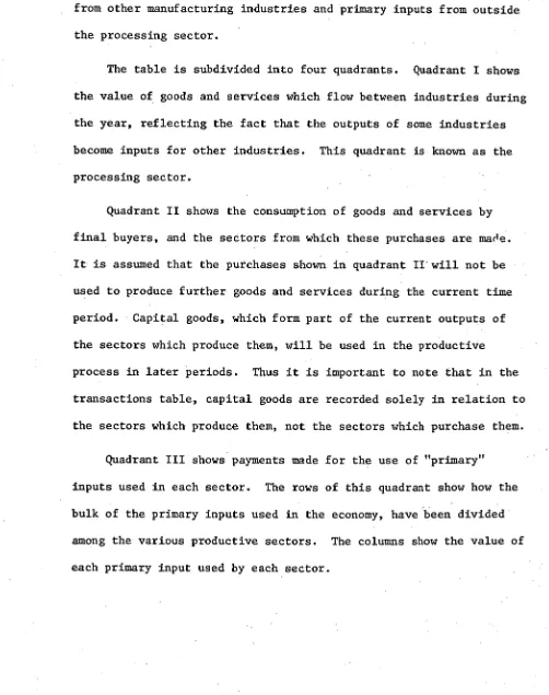
Figure 2-1 shows the normal layout of a transaction table.

Each row in the manufacturing or processing sector shows the

distribution of the output of that industry to other manufacturing

industries and to final demand. Each column of the processing

sector shows the industry's input purchases - intermediate goods

from other manufacturing industries and primary inputs from outside

the processing sector.

The table is subdivided into four quadrants. Quadrant I shows

the value of goods and services which flow between industries during

the year, reflecting the fact that the outputs of some industries

become inputs for other industries. This quadrant is known as the

processing sector.

Quadrant II shows the consumption of goods and services by

final buyers, and the sectors from which these purchases are ma0e.

It is assumed that the purchases shown in quadrant Irwin_ not be

used to produce further goods and services during the current time

period. Capital goods, which form part of the current outputs of

the sectors which produce them, will be used in the productive

process in later periods. Thus it is important to note that in the

transactions table, capital goods are recorded solely in relation to

the sectors which produce them, not the sectors which purchase them.

Quadrant III shows payments made for the use of "primary"

inputs used in each sector. The rows of this quadrant show how the

bulk of the primary inputs used in the economy, have been divided

among the various productive sectors. The columns show the value of

Figure 2-1 QUADRANTS OF THE TRANSACTIONS TABLE

PROCESSING SECTOR

II FINAL DEMAND II _II II OUTPUT TO --->

INPUT FROM / 0 ca. 0 0 1-. 0 ci 0 0 PO

01-I

ra.

g 4

I-I 0 a o U) 4 0 0

A

A

(DO _{Q. 9}

1-.. 0

rt r+

g g CD 1

P.

l*

‘C

0

.3 _CD

CA

5

a C.!.

II 0 P. 0 0

° .11 _P.

fir

I-.

4

I I n 0 ICI Irl 11

>

8

A A li ig 11 8

5 . 1 a la 11 '' _{0 I 1 II}

1--. < II-I 10 II P3 CD 10 IC II 0

prt 4 ig 14 11 9

0 0 11 to et Pu

° 14 IA 11 9

IP) ID) II 14-1. 1 11 I CD 1 II

I I II

7

0 z

g--4

w

Cl)

t

ri 0

0 X

;

'Ti Industry 1

Industry 2

•

Industry i

Industry n

•

-

I I I II Quadrant II1 1 1 11^, 1 u v

F 1

+

_ _

_ F _

_ _

I

I

r 1- -- -

P 1

g t 1 ItX

o p o

I 1 1 1 11 1 I I I I II I I I 1 I II I- - - - -I- - - - -I- - - - -11- - -I- -714 - - - s ; 1 1 i 11

1 o 1 1 IOC 11 1

r r r r r -ff - - - 1 1 1 I I II 1 1 I I 1 II 1 I 1 1 1 II I I I 1 I II

r r

P g g 1 1 II

1 o 1 t 1 uX ; t i 1 i u -n

1 1 to it En E-4 174 I ; 11 a cc z

Wages 1 ;Quadrant III 1 Quadrant IV

r— r -ft

Gross Operating

Surplus

Depreciation

Payments to Public

Authorities Imports Interstate Imports Overseas TOTAL PAYMENTS I — A - i I 1:2 1 I $ I I , g >4 • 1' •1 --- 1 $ g t 1 g g $ g g 1 1 I g g g g g g 1 t 1 -- -- -1 ---1 - --f .--/ ---1 --- 1 g g t g g g 1 1 g r---- I-1 -- I-I ---- 1- ---+

1

--(7 , - 1 1-- --- 1-F -- 1--- 1----1+---- I I I I [ II X 1 I I ■ 1 i t i II - - - = ,

t 1 11 i ; s t i II I 1 1 1 I II i 1 1 i 1 II i 1 I II

1 ; i 1 1 II

r r----r----r--r--m--- I t i i i II

i t ; II g II

1 1 I 1 I II -1.----,----_,--- 1---1.--*---

, o i t 1 11 t 1 I p i 11

--,-r----t.,v,,r,r,-w.-- I i I i 1 11 1 p t p I II

---- ...L....14... I I . I 1 11

Quadrant IV shows the primary inputs which pass directly into

final use, such as imports of consumer and capital goods, and direct

employment of labour by households and non-trading government

departments.

As has already been shown, corresponding rows and columns of

industries within the processing sector must balance. There is,

however, no necessary correspondence between the total of any row or

column outside the processing sector. The row values of primary

Inputs and the column values of final demand are merely required to

balance in total.

2.1.2 Mathematical Relationships

LetLbe the total output of industry i where 1=1, n 1

referring to the n endogenous sectors of the economy.

Let x

ij represent the amount of output industry i sold to

industry j and which is used as an input in producing X.

Let D

i be the final demand for output of industry i, that is

the sum of the output of industry i sold to the final demand sectors.

LetV.be the value added for industry j, that is the sum of

the payments sector for industries.

For a particular producing industry i, the total output, X i , of

that industry can be distributed among the various industries and

final demand component as follows:-

X

D 1

D 2

D. • •

,11■111.1.

7.

Thus, distribution of output between intermediate and final

demand can be expressed as

X

i xij + Di

j=1

, n) (2-1).

For a particular consuming industry j, the total output of that

industry will be equal to the sum-of total inputs (from other

industries) plus payments made in the value added sector.

Xj = xij + x2j +... x + xnj + Vj

X. = x.. + V (j=1,

i=1 13 j

The whole system can be represented in matrix form.

x

11 x xi 12 lj xin

x

21 x22 • • x2j x 2n

•

x_il

•

x ...x .'...x.

.i2 ij in

• _•

dr■■■• 1111■101■., x

nl xn 2 xnj x nn

.

E7 •••

• 2

1 X2

2.1.3 The Table of Technical Coefficients

The technical coefficient of production may be defined as the

amount of output from industry i required to produce a unit of output

of industry j.

i.e. _{a.. - xii}

8.

Thus each x.

j in the transactions table may be expressed as a

i

productathetechnicalcoalicienta.

j and the total output of

i

sector j.

x.. = a. .X. (2-2)

13 133

The technical coefficients may be written in matrix form as

follows:-

••••■■■

a12 ••• a

lj ... a ln

a

21 a22 a2j a2n

• . . .

• • . .

. . • a

il a i2 ij *Oa a. ... a. in . .

. .

. . . . a

nl an2 ... a j ... a nn

■•■•••■

For an industry j, the technical coefficients show the amount of

direct purchases required, from other industries, to increase thr

value of output of industry j by one dollar.

2.1.4 The Table of Interdependence Coefficients

The increase in direct purchases of inputs required to meet an

additional dollar output of final demand does not represent the

overall addition to total output. The increased purchase of inputs

from other industries, requires these industries to purchase

additional inputs to meet their increased output. A chain reaction

of stimulated indirect production takes place throughout the

processing sector.

The combined direct and indirect effects can be calculated by

an iterative procedure but in practice this is not possible except

for very small matrices. The alternative method is to use the

general solution for an input-output model. a

9.

By substituting a..X. forx ij in (2.1), the technical conditions

13 J

of production can he written as:-

X.=ia..X.+D.for i=1, n

1 ij

j=1

or in matrix form

X = AX + D

X - AX = D (2-3)

From (2-3), the relationship between an exogenousiy determined level

of final demand and the total production (including intermediate

production) required to produce- that final demand can be derived:-

X(I-A) = D where I is the nxn identity matrix

X = (I-A)-1D where (I-A)-1 is the general solution

= BD (2-4)

Eachelement,b.., of the matrix B represents the sum of the direct ij

and indirect outputs of industry i required by the economic system

in order to deliver a dollar of additional output of industry j to

the final demand sector. The matrix B is known as the table of

interdependence coefficients.

2.1.5 Stability Conditions

The stability conditions set out the mathematical requirements

which must be met by any workable input-output system.

(a) Table of Technical Coefficients

(i) at least one column in the table add up to less than unity

(ii) no column in the table add to more than unity (which

merely implies that no industry can pay more for its

10.

(b) Table of Interdependence Coefficients

(i) there can be no negative entries. 1

•A negative entry would mean that each time the industry with a

negative entry expanded its sales to final demand, its direct and

indirect input requirements would decline. That is, the more the

industry expanded its output the less it would have to buy from

other industries, clearly an economic contradiction. This condition

is directly comparable to the linear programming requirements of

non-negativity of activity levels.

These conditions are useful checks in the compilation of an

input-output study. They are a means of detecting whether or not

an error has been made in collecting or assembling data.

2.2 The Assumptions

The system described above is the open static model which is

the basic (and still the most frequently used) form for input-output

analysis. Before looking at extensions to and variations of this

basic model, it is necessary to outline the assumptions of the basic

model.

The essential assumptions of input-output theory are concerned

with the nature of production. The unit of investigation is the

industry which may consist of many individual firms.

It is assumed possible to group the productive sectors of an

economy, such that, a single production function can be determined

for each industry formed. Corollaries of this assumption are that a

I Known as the "Hawkins-Simon Condition" The mathematical proof is developed in [17]

11.

given product (which for empirical work may be a group of r:ommodities)

is only supplied by one industry and that there are no joint products.

Each industry is assumed to have a linear production function

which is homogeneous of degree one. When the level of output is

changed the amount of all inputs required is also changed in the same

proportion i.e. constant returns to scale. The general form of the

production function can be represented by

X. = f(x

lj, x2j'' xij' xnj)

Entries in the same column of the transaction table are the inputs of

the same production function.

Input-output economics makes a further strong assumption about

the nature of production - there is no substitution among input

factors. Fixed coefficients of production are a characteristic of

the fixed-proportion production function - a limiting case of the

traditional homogeneous production function of degree one. A certain

minimal input of each commodity (possibly zero) is required per unit

of output of each commodity. This special production function is

represented by

x.. X = mm (—u- ±?-1-1

lj a 2j a. ij

SOO

a 8)

nj

where the notation min (a, b, z) means the smallest of the

numbers a, b,

Since X. equals the smallest of the input ratios

x.,

then X. 45 j=1, n; i=1, n

j a. ij

12.

'However, in drawing up the transaction table only scarce commodities

are tabulated as inputs (i.e. free goods are not considered). As it

is reasonable to assume no rational industry would use any input

beyond the minimum requirement then output reduces to the equality

of equation (2-2)

xij . = a..X. j j=1, n.

Each input is required in fixed proportion to output.

With this type of production function there is only one

efficient way to produce any given amount of output. The isoquant

surfaces are thus nested right-angled corners.

xii

=

x2i

This is a radical departure from conventional production theory

where homogeneous production functions of degree one are assumed to

have inputs which are continuously substitutable and the technical

marginal rate of substitution between inputs diminishes. Ignoring

such production possibilities would appear to be a serious

limitation for input-output tables for the purposes of analysis and

prediction. However, the assumption of discontinuous substitution

can be defended in empirical work by the judgement given by Cameron

13.

activity is characteristically not a choice between continuously

substitutable factors (which can be solved by the equi-marginal

productivity condition), but a choice between a finite number of

methods of production with each of which is associated certain

capital equipment and fairly closely specified rates of flows of

inputs."

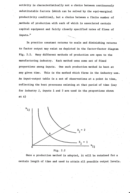
In practice constant returns to scale and diminishing returns

to factor output may exist as depicted in the factor-factor diagram

Fig. 2.2. Many different methods of production are open to the

manufacturing industry. Each method uses some set of fixed

proportions among inputs. One such production method is best at

any given time. This is the method which firms in the industry use.

An input-output table is a set of observations at a point in time,

reflecting the best processes existing at that period of time (say

for industry J, inputs 1 and 2 are used in the proportions shown

at A)

Fig. 2.2

Once a production method is adopted, it will be retained for a

14.

Output thus expands or contracts along the scale line OA.

Cameron [4] in a time series analysis of selected input coefficients

in 52 Australian industries, concluded that his results generally

supported the assumption of fixed production coefficients in the

short run.

However, eventually the production process changes and

consequently technical coefficients change. Improved technology is

recognised as the most important factor responsible for altering the

technical coefficients (particularly so because technological change

is also responsible for most of the changes in relative prices of

inputs). Thus it is advisable, that complete or partial revisions

of input-output tables be made at time periods of around five years.

A further assumption of the input-output model is that the

total effect of carrying on several types of production is the sum of

the separate effects. This is the additivity assumption (also an

assumption of linear programming models) which rules out the

possibility of external economies and diseconomies. This assumption

is important in calculating projections. The total of any output

needed to produce an assigned target of consumption goods can be

built up by adding the separate outputs needed to produce each item

of the target.

2.3 Variants to the Open Static Model

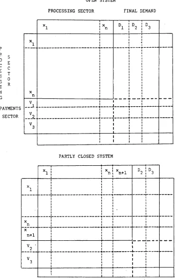
2.3.1 The Closed Input-Output System

The open system described earlier may be closed with respect to

one or more of the sections in the final demand sector, by making

15.

The most common form of closed system incorporates the personal

consumption section of final demand as a productive sector. The

consumption of goods and services becomes the industry "Households"

the output of which is represented by payments to households, that

is wage and salary payments (see Figure 2.3). Tables of technical

coefficients and interdependence coefficients are formulated for

this closed system in the same manner as for the open system.

This system has a close resemblance to the aggregate multiplier

of the Keynesian income-consumption theory. Given a change in final

demand, the open system is capable of evaluating only the direct and

indirect effect on output requirement. However, changes in output

levels lead to changes in income which in turn induces changes in

consumption. Therefore, only part of the overall impact of a given

change in final demand can be evaluated from an open system whereas,

the closed system may be used to evaluate the direct and indirect

effects of the open system plus the induced changes in income

resulting from increased consumer spending.

For some analytical work the system is closed with respect to

exports and imports - in other cases both households and foreign

trade are incorporated in the closed system.

It is also possible to shift an industry, normally included in

the processing sector, to the autonomous final demand sector. This

technique is used when an analysis is required of the inter-industry

effects of changes in the level of activity of the particular

industry. The extent to which an input-output system is open or

•••■•••••••■■•••• •••••.'•-•P••••••

D 2 I D3

x n

n+1

4... A- -11-

V 2 •

V 3

OPEN SYSTEM

PROCESSING SECTOR FINAL DEMAND

P

0

PAYMENTS SECTOR

x i _xn D

1 D2 D3

1

-

- -

"1-

- — -

V

V 3 V

2

...

4

PARTLY CLOSED SYSTEM

Section D

1 of the exogenous final demand sector has been made industry x

n+1 of the endogenous processing sector.

16.

17.

The additional sectors made endogenous by closing a system,

are also subject to the assumption of fixed coefficients of

production. The coefficients associated with consumption, however,

are behavioural rather than technical and, as a consequence, are

not as stable as the true technical coefficients of a manufacturing

industry. Therefore when using a closed system, the consumption

coefficients must be revised more frequently than the technical

coefficients of an open system.

2.3.2 The Dynamic Input-Output System

The static model is based upon current flows and current

output and because of its fixed technical coefficients, it is

limited to short run analysis. In recent years much of the research

in the field of input-output economics has been directed towards

the development of dynamic models aimed at long term analysis. The

production of current inputs in one period is proportional to the

output level of that period but, by contrast, the amount of capital

. goods produced is related to production in later time periods. The

link between intertemporal models is achieved by using the

acceleration principle which relates capital investment to changes

In the level of output capacity'.

In the static model, capital formation is recorded as a

• sector of final demand and recorded in the column Domestic Capital

Formation. Capital is thus treated as a stock concept in contrast

to the flow concept of goods and services within the processing

sector. Where sufficient data are available in an economic system,

it is possible to construct a capital transactions table. The

layout of this table is similar to the transactions table of goods

INTERINDUSTRY TRANSACTIONS TABLE

18.

1 xln S1 xl

PC

xii _xij xl

n

,

.

.

.

xl

_1x

INTERINDUSTRY CAPITAL TRANSACTIONS TABLE

Sector S of Final Demand represents Domestic Capital Formation.

x

1 I

k

r1

1,71

s ii

i

1

s

_{11 i}

. I

ij

1

S

n f Snn

S .

1 i Sj

x

₁

x

n

S i

S i

Theelements.

j of l the matrix S may be defined as the quantity of capital goods produced by industry i and sold to industry j.

Each row of the Capital Transactions Table shows the 'disposal

pattern of capital goods produced by a particular industry. Each

column shows the source of capital goods purchased by a particular

19.

Average and Incremental Capital Coefficients

Theaveragecapitalcoefficient,k_may be defined as the ij'

amount of capital. goods produced by industry i and required by

industry j per unit of output of industry j

i.e. k = sij .

X

i

The matrix K, of average capital coefficients, is used for

structuralanalysis.TheK.

j 's show the amount of capitalrequired

i

per unit of output of an industry.

Fordynamicanalysis,incrementalcapitalcoefficientsa.are ij

required. These coefficients show the amount of capital required

per unit of increase in output capacity of an industry between two

time periods.

.,

ere AX

Ak. = _lj where s1.1 = X. - X.,t

j j,t+1 _J

AX i

Intertemporal models are linked by means of the matrix of

incremental capital coefficients, K.

Requirements of the Dynamic Model

The data demands of the dynamic model are enormous and at the

present time, theoretical development is well in advance of

empirical application so that the dynamic input-output model lies

at the frontier of current knowledge.

The construction of a general dynamic interindustry model

requires a partly closed system incorporating income generation, a

complete description of the capital structure of the economy to

provide investment accelerators and some means of estimating

20.

alternative production techniques. This latter aspect may require

linear or non-linear programming studies of firms within an industry.

A less rigorous, but intuitively appealing approach has been

developed to incorporate technological change into dynamic models.

New technical coefficients computed from a sample of "best practice"

firms in each sector are substituted into the inter-temporal models.

The underlying assumption is that at any given time, some firms in

an industry are more advanced than others. The input patterns of

these "best-practice" firms in an industry can be used to project

what the average input patterns of that industry will be at some

time in the future.

21.

CRAPTER 3

ECONOMIC ANALYSIS WITH INPUT-OUTPUT MODELS

3.1 Input-Output and Economic Development

Input-output economics provides analytical methods which can be

applied to any kind of economic system during any phase of its

development. The form of economic analysis is positive rather than

normative in that it deals with what

is or what will be

to

what ought to be.

optimising technique.

All the various forms of analysis of input-output economics deal

in terms of the final demand for goods and services and the

inter-industry transactions required to satisfy that demand for an economy

in equilibrium. Thus, the input-out2ut method is a form of consistent

equilibrium analysis.

The transactions table of an input-output model gives a detailed

quantitative description of the industrial structure of an economy with

respect to the year for which it is compiled. Although such a

dis-aggregated presentation of national accounting could of itself be of

some value in policy formulation, the real value of the input-output

method lies in its capacity to analyse practical problems relating to

industrial structure and to devise and test economic policy.

Economic development is brought about by the formation of a high

level of interdependence within an economy. Higher real per capita

income is achieved through industrialisation and a build up of the

related tertiary activities. The shift in employment from primary to•

secondary and tertiary sectors means that the economy has to undergo

22.

by the use of analytical techniques to formulate economic policies

which encourage strong structural interdependence within the economic

entity. The input-output method is such a technique which is now

widely used in the analysis of economic development, short-run

fore-casting, and simulatiop experiments on structural and policy changes

for an economy.

The aim of this chapter is to outline some of the methods of

economic analysis which may be applied to the transaction table

compiled for this study. Some of the analytical techniques have been

performed and are presented in Chapter 6, others may be performed in

subsequent studies.

The methods fall into two broad categories, qualitative and

quantitative analysis.

3.2 Qualitative Analysis

Structural Analysis

In a transactions table where the position of an industry in the

table is arbitrarily assigned, hierarchial interindustry relationships

may be obscured. Triangularisation is achieved by re-arranging the

rows and columns so that, starting from the top of the transaction

table, the rows are placed in descending order of the number of zero

entries across a row. In a strictly triangular matrix, industries

below any given row are that industries suppliers while the industries

above that row purchase the given industry's output.

While symmetrical triangularisation is rare, re-arrangement from

random ordering of industries towards triangularisation, simplifies

the task of identifying interdependence within the economy. Industries

near the bottom of a triangularised table have strong interdependence

23.

Industries near the top of the table have strong interdependence on

the input side and therefore have a high multiplier effect upon the

rest of the economy when final demand for their product is increased.

In planning future developnent these latter industrie; are the

industries to be encouraged. The interindustry effects set off by

their growth generate expansion in all sectors of the economy.

Triangularisation of successive tables is important for making

intertemporal comparisons of the productive structure of an economy

in order to examine the rate at which strong interdependence is being

attained.

The Self-Sufficiency Chart

This form of analysis, explained and illustrated with empirical

examples by Leontief f25] in his Scientific American article, makes

use of three indicators of interindustry production levels to examine

the external trade of an economic entity:-

(a) the amount of production that would be required from each

industry to satisfy the direct and indirect demands of the

domestic economy if it were to achieve self sufficiency

(b) the direct and indirect requirements of each exporting

industry in order that its exports be produced entirely

from domestic resources

(c) the amount of production, both direct and indirect required

from particular sectors to producer goods that are

currently imported.

While the development of strong industrial interdependence is

important in the pursuit of economic development, the advantages of

specialisation and exchange must be acknowledged together with the

24.

However, increases in sufficiency usually are. The

self-sufficiency chart form of analysis projects changes which will have to

be brought about in groups of structurally related industries as the

economic entity moves towards the degree of self-sufff.ciency where

non-replaceable imports are covered by the exports ncleded to pay for

them. That is, the projections indicate where policy guidance could

help bring the economy towards the level of self-sufficiency where

exports and imports balance on current account.

3.3 Quantitative Analysis

Multiplier Analysis

The macro economic and employment multipliers, developed from

Keynesian theory, deal in the broad aggregates of the economy. The

multipliers of input-output analysis deal with the impacts that

individual industries exert throughout the economy and are thus

supplementary to the aggregative multipliers. By dividing an economy

into finer units, input-output analysis is capable of examining

effects undetected in general macro analysis.

Industry multipliers were devised in a regional study by Moore

and Petersen [31] and developed by Hirsch [18] in a later small area

study. Multiplier analysis has become the most important technique

used in regional economic impact analysis. Impact studies are

concerned with changes in the parameters of an economy such as changes

in final demand or a change in input structure of one of more

industries. Multipliers relating to output, income and employment may

be calculated from the input-output model together with the direct,

indirect and induced components.

The output multiplier is the sum of the columns of the open

25.

industry J is h.. and represents total requirements (direct and ij

indirect) per dollar of final demand.

In order to calculate income multipliers the system is closed

with respect to "Households". The Type 1 income multIplier is the

ratio of the direct plus indirect income change to the direct income

change resulting from a dollar increase in final demand for any given

industry. The direct income change for a given industry is the

entry in the Households row of the table of technical coefficients

(let Matrix A including Households be A*). The direct and indirect

income change is calculated for each industry by the vector-matrix

multiplication of the row vector for households in the A matrix and

the column entries for each of the industries in the open Leontief

inverse matrix.

n .

. A* b. (j

i=1 Hj ij n)

The calculation of Type II multipliers requires the generation

of a Leontief inverse matrix for the system closed with respect to

households (i.e. the B matrix). The households row of this matrix

gives the direct, indirect and induced income changes per dollar change

in final demand and is known as the regional income multiplier. The

Type II multiplier is the ratio of the direct, indirect and induced

income changes (regional income multipliers) to the direct income

change.

Employment multipliers similar to the income multipliers may be

calculated from the input-output model and are valuable to planners

interested in the employment effects of changes in industrial output.

The simplest forms are where employment is assumed to be directly

26.

Jensen [21]. The direct employment coefficient (e) for each industry

J is calculated as the number of employees per $1,000 of output of

industry J

e. = X. (in $'000) j

E. 3

wherex.isthevalueofinclustrydutputandE.is the industry

employment level in man years. The direct plus indirect employment

change is calculated by multiplying the row vector of direct

employmentchangecoefficients(e.)and the corresponding column

entries of the open inverse matrix B and summing the resultant

products, i.e.

e. b. j

i=1 3 13

•• • , n

The calculation of the direct indirect and induced employment

change is similar but the closed inverse matrix B * is used, i.e.

e. b. j = i=1 3

•• • , n

The Type I employment multiplier is the ratio of the direct

plus indirect employment change to the direct employment change.

The Type II employment multiplier is the ratio of the direct,

indirect and induced employment dhange to the direct employment change.

The above employment multipliers assume A linear homogeneous

employment-production function which is likely to be an over-estimation

of the real values. More accurate employment multipliers can be

produced when sufficient data exists to estimate curvilinear

27.

Projection and Simulation

Economic projection is one of the principal uses of input-output

analysis. The objective is to measure the impact on the economy of

autonomous changes in final demand. By decomposing au economy into

finer units, input-output forecasting is capable of tracing out

effects undetected in general macro-analysis.

For an economy operating under the market system, the final

demand sectors are regarded as autonomous. The levels of final demand

in a future time period can be estimated by econometric techniques.

Input-output forecasting is aimed at determining the levels of activity

which will have to be attained within the endogenous processing sector

In order to sustain the estimated level of final demand. This is

termed "consistent forecasting", as the output of each industry is

consistent with the demands, both final and from other industries, for

its products.

The projection method is based on the mathematical relationships

established in Chapter 2. After estimating the projected level of

final demand in appropriate industrial detail, the final demand sectors

are aggregated to form a new final demand vector, say D'. Using the

equation (2.4) X = BD a new vector of total output, X', can be

obtained:-

X' = BD'.

The levels of activity within the processing sector of a new

transactions table can be established from the equation

(2.2) xij = a..X.

1J J

1

so that As Vt 4

1—=1, .41.9 n; j=1, 000, n.

1j = n_{JJ J}

The transactions table is completed byl disaggregating the final

28.

Using computers and mathematical software packages the matrix

multiplication involved in making projections can be calculated very

simply and rapidly. The transactions table thus becomes a model of

the flow of goods and services within an economy suitable for

simulation studies and sensitivity analysis.

Structural simulation tests can be used to examine the effects

of changes in exogenous variables (such as changes in the level of

exports) and endogenous variables (such as adding new industries

or removing existing industries). Policy simulation demonstrates

the effects of government fiscal and monetary intervention in the

economy, on such matters as increased government spending in

particular sectors, changes in the level of consumer spending

induced by changes in direct and indirect taxation and transfer

payment. Simulation for policy determination can be performed more

efficiently where price and income elasticities of demand have been

determined.

Simulation experiments are of particular value to public policy

makers when employment is linked to the monetary transactions. The

simplifying assumption may be made that employment is directly

proportional to the level of output in each industry. The direct

employment coefficients described earlier may then be used to

calculate the employment levels of new projected output totals for

industries. If separate estimations of the exact relationship

between levels of output and employment exist, then these equations

can be used in lieu of the proportionality assumption. In either

case estimations of employment levels on an industry basis, can be

29.

CHAPTER 4

REGIONAL INPUT-OUTPUT MODELS

4.1 The Development of Regional Models

The initial theoretical development and early empirical

application of input-output economics dealt with a national economy.

From the late 1940 1 s there developed an accelerating upsurge in

regional economic studies and input-output was quickly adapted to

the regional level. Over the years, due to improved official

statistics collection, the development of new compilation techniques

and the proliferation of computer facilities and capacity,

input-output analysis in some variation or form has assumed a dominant

position in regional research.

The variety of regional models, which have been both formulated

and applied, fall into the two broad classifications of

inter-regional and single inter-regional models. The former models take account

of inter-dependence between regions as well as industries. As a

consequence they are more complex than the latter models which

closely resemble national models but refer to a smaller economic

entity.

The inter-regional models have developed from two different

concepts. The balanced regional model formulated by Leontief [26 Ch.9]

used a national input-output table and disaggregates this into

regional components. The two or more regions produce regional

commodities consumed within their region of origin and national

30.

The pure inter-regional model proposed by Isard [22] developed

a national table by aggregating a number of regional tables. The

balanced regional model has had greater success in empirical

application, though from the inception the two systems were not

viewed as alternatives but complementary with the balanced regional

model serving to determine regional implications of national

projections and the pure interregional model estimating national

implications• of regional projections.

Generally, the empirical application of inter-regional models

has been restricted by the lack of information on the flow of goods

and services between regions. Inter-regional modelling was an

ambitious concept to be attempted so early in the development of

input-output economics but reflects the long felt desire of regional

researchers to identify and quantify inter-regional transactions.

Current inter-regional studies have .a higher probability of

accurately identifying these transactions flows due to the better

data, methods and facilities mentioned earlier.

The early single region studies also suffered from a dearth of

regional statistics. As an expedient, the compilers of both

inter-regional and single region studies were forced to assume that

coefficients from national input-output tables applied to the

inter-industry flows within a region. Total gross output figures for each

sector were assembled from published data and the national

coefficients used to calculate the regional transaction table.

Thatis,thea.elements from the national table of technical ij

coefficients were multiplied by the regional industry output total,

X. to give the regional flow of goods from the i-th to the j-th

industry,

r .

x.. = a..X. (1=1, n; =1, 6", n)

j

31.

This assumption imposes a severe limitation on the use of such

input-output tables for analytical purposes.

The single regional models may be broadly classed into those

using surveys and those using non-survey techniques. Of the latter

the simplest method involved representing the regional economy by

essentially, unmodified national technical coefficients. In Australia

Mules [31] used this procedure to construct an input-output matrix for

South Australia.

The input-output study of Utah by Moore and Petersen [31]

achieved a breakthrough from the practice of using unadjusted national

coefficients in a regional model. A transaction table calculated by

the above method was regarded as a first approximation. Then "the

row and column distributions for each sector were modified in the

light of differences in regional productive processes, marketing

practices, or product-mix" [31 p371]. Statistics relating to exports

and imports for the State of Utah were not available. The local

inter-industry flows, for each inter-industry, were identified by deducting from

the estimates of gross output the estimated demand in Utah. A positive

residual was treated as an export and a negative residual as an

import. This procedure assumes that input requirements are used first

from locally produced goods. •This assumption is severely criticised -u

by Tiebout [42 p145] because it "can lead to some ridiculous results

in determining net exports and imports."

Since regional coefficients are known to vary considerably from

national coefficients, the use of unadjusted national coefficients is

undesirable. The largest source of variation between regional and

national coefficients arises from the greater openness of regional

32.

be greater at the regional level than at the national level.

A variety of adjustment techniques have been devised of which the

R A S method is the most widely used.

The first survey-based regional table was produced by Hirsch 118]

in a study of a small geographical region (the St. Louis Metropolitan

area). Hirsch was able to identify more accurately exports and

imports, as well as interindustry flows, by personal interviews and

sample survey. Using these methods it was possible to identify the

region's exports and imports beyond mere totals for each industry.

In the final tabulation of the St. Louis study, the rows identified

not only the regional distribution of interindustry sales but also

the distribution of sales to specific industries outside the region

(i.e. exports were disaggregated). Similarly, the columns identified

the interindustry inputs from within the region together with inputs

from specific industries outside the region(i.e. imports were

disaggregated). The accuracy achieved by this type of study is

obtained at very high cost and consequently the method is suitable

only for small regional studies.

A hybrid approach, balancing the cheap but potentially unreliable

non-survey approach with the cost-prohibitive survey method, is

advocated by Richardson [41]. National coefficients are least

appropriate to use for primary industries and industries in which the

region specialises and surveys are required for accurate estimation.

Some geographically isolated regions record both production and

trade data. Exports and imports of the region may be simply recorded

as total trade or broken into foreign trade and trade with all other

regions of the nation. For such regions, it is possible to construct

33.

and with accurate import-export sectors. Parker [34] was able to

make such a study for Western Australia.

4.2 Australian Input-Output Studies

Although input-output tables have been compiled on a regular

basis in a number of countries, Australian use of input-output

analysis has not been extensive until recent years. Australian

research began early in the era of input-output work with the

construction of national tables by Cameron [6] for the year 1946-47.

The production of national tables has since been taken up by the

Commonwealth Bureau of Census and Statistics with the initial

publication in 1964 of tables for 1958-59 [8]. This first table

was regarded as experimental and made no attempt to gather data

beyond that which was readily available. For the 1962-63 tables

published in 1973 [9], more resources were used together with

supplementary inquiries to augment the regular data collections.

The 1968-69 tables published in 1976 [10] have a similar industry

structure to the 1962-63 tables and for the purposes of analytical

work are compatible. The Bureau now plans to produce national

tables every five years.

The first State input-output study, that of Western Australia,

was made by Parker [34]. The compilation of this table followed

more closely that of a national table rather than regional in that

commodity data of the factory censuses formed the basis of

construction. Input-output tables for South Australia, based on

adaption of the 1958-59 national coefficients, were tabulated by

Mules [33] and used for the analysis of a particular industry sector.

The first small scale regional model was published in 1969

34.

economic structure of the town of Muswellbrook in New South Wales.

Since that time there have been a number of town or city

input-output studies compiled by survey work. These included Gatton (Qld)

by Reynolds [40] and Tamworth (N.S.W.) by Percival [39] where the

partial input-output method of intersectional flows was used.

Harvey [16] produced an input-output model of the Darling Shire to

examine the effects of the 1969-70 wool price slump on the economy

of the township of Bourke. McGaurr [30] constructed input-output

tables for Toowoomba with 9 of the 15 processing industries estimated

from survey data with 2 industries estimated exclusively from

secondary data.

Two sub-State, large regional studies have recently been

completed by Jenson [23] with Central Queensland and Mandeville [28]

with the Macquarie Region of New South Wales, both based on field

work with questionnaires. The first inter-regional study in

Australia is currently being prepared by a research team, led by

members of the Department of Economics, University of Queensland [24].

Other input-output tables currently under construction include a model

of South Australia by Butterfield, the Illawarra Region by Ali and the

Townsville Region by Dickenson.

4.3 The Need for a Tasmanian Regional Study

In a report [35] presented to the Tasmanian Parliament on the

occasion of the 1970-71 Budget, the Treasurer expressed concern that

Tasmania's economic performance, in the pursuit of economic goals,

compared unfavourably with that of mainland States and the overall

Australian achievement. The objectives of economic policy in

Australia have appeared from time to time in public documents and

35.

A high rate of economic growth

A high rate of population growth

Full employment

Increasing producAvity

Rising standards of living

External viability

Stability of costs and prices

Although, over the last decade, the level of achievement at a

national level may have vacillated, at State levels there has been

even greater variation, and in addition, widely differing rates of

attainment of objectives between the component States have been

observed. Indices which provide measures of regional prosperity

currently suggest that Tasmania still does not measure up to the

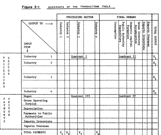
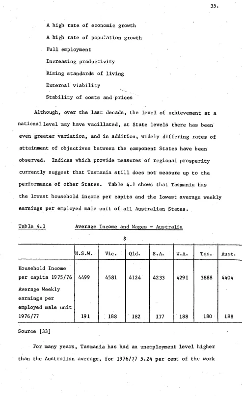
performance of other States. Table 4.1 shows that Tasmania has

the lowest household income per capita and the lowest average weekly

earnings per employed male unit of all Australian States.

Table 4.1 Average Income and Wages - Australia

N.S.W. Vic. Qld. S.A. W.A. Tas. Aust.

Household Income

per capita 1975/76 4499 4581 4124 4233 4291 3888 4404

Average Weekly

earnings per

employed male unit

1976/77 191 188 182 177 188 180 188

Source [33]

For many years, Tasmania has had an unemployment level higher

36.

force as against the Australian figure of 4.99 per cent.

Regional studies have indicated that a disparity in regional

prosperity is prevented from growing to large proportions by the

balancing mechanism of population drift, i.e. out-migration takes

place from relatively depressed regions and is directed towards

areas of better employment opportunities.

The net migration figures for Tasmania, indicate that the

balancing mechanism operates. Despite a higher than average birth

rate, Tasmania has a low rate of population growth by comparison

with the rest of Australia. This can be attributed to the very low

net migration figure for the State which in some years is actually

negative. A significant feature of the population drift is that most

out-migration appears to emanate from the 15-24 year age group, the

new entrants to the work force.

The Draft Report of the State Strategy Plan [37 p10] has

commented " the recorded unemployment in Tasmania at the end of

June 1976, of about 9,000 persons, does not represent the true position.

The migrants from Tasmania of working age should be considered as part

of the unemployed of Tasmania. If they were to return immediately then

there would not readily be employment for them. The true unemployment

situation is closer to 11,200 unemployed, or nearly 6.2 per cent of the

work force".

While the objective of a high rate of population growth has

currently become controversial in some States it remains an important

• objective for Tasmania. The small Tasmanian population impedes economic

development in that the domestic market is too small for many industries

to achieve competitive economies of scale in production. High

37.

Tasmanian based industries to attain viable size by means of

interstate marketing.

Apart from deterring the establishment of new industries,

the interstate shipping rates have actually prompted a number of

established firms to relocate on the mainland and others to

under-take comparative cost studies to examine the feasibility of

re-location.

The drift of potential work force participants has resulted in

Tasmania being the State with the lowest proportions of population

in the working age group 19 to 64 years. The Grants Commission

[12 p8] has commented that this is one of the factors which may

contribute to a State's comparatively low fiscal capacity.

The rural sector is also beset with serious problems. Along

with the rural industries of all other States, the rural industries

in Tasmania are being forced to restructure. By comparison with the

more populous States, Tasmanian farm reconstruction may well have a

greater impact on the economy of the State. Farm size is small, the

proportion of the work force engaged in rural production, 9.0 per

cent, is greater than the Australian average of 7.3 per cent (1971

Census figures) and most rural industries are more export oriented

than the overall average for corresponding Australian industries.

Two major rural industries, fruit growing and dairying are facing

severe marketing problems for their products and industry contraction

is taking place. Will the displaced farm operators and farm workers

be provided with employment in the State, or will an accelerated

drift towards interstate migration take place?

To what extent will changes in farm size and farm population

38.

In order to reverse what appears to be a trend towards economic

stagnation, special policy measures are required to stimulate economic

growth. These economic policies call for special economic

analytical and planning pro -:edures. An input-output study is a

contribution towards this requirement. Despite the limitations

imposed by the simplifying assumptions detailed in Chapter 2 and the

problems of data deficiency outlined in this chapter input-output,

with its rigid organisational framework and accounting consistency

39.

CHAPTER 5

PROCEDURE AND DATA SOURCES

5.1 The Integrated Censuses

The financial year 1968-69, the year of the first integrated

census in Australia, was selected for this study. The integrated

economic census has been the most important development affecting

the quality of statistics compiled by the Australian Bureau of

Statistics (ABS). The integration of censuses for manufacturing,

mining, wholesale and retailing has meant that for the first time

these censuses have been collected with a common framework of

reporting units and data concepts and conform to an international

standard industrial classification. The Australian Standard

Industrial Classification (ASIC) [10] follows the principles used

in the United Nations Industrial Standard Classification of

objective coding of establishments to industry classes according to

the nature of the detailed output of commodities and services

reported by them.

The integrated censuses provided a far more comprehensive and

consistent set of data for this study than had been available for

earlier input-output studies in Australia. The integrated censuses

were initiated by the demand for statistics suitable for economic

studies, including input-output, the data needs of which were taken

into account in the design of the censuses. The structure of the

census analysis was directed towards the derivation of the more

internationally accepted "value added" instead of the former concept

40.

instead of the value of output at the factory and purchases and

selected expenses in addition to the value of specified materials.

Large companies with a range of manufacturing a:tivities were

treated as being composed of several separate establishments. For

instance, the mining operations of Electrolytic Zinc Company of

Australasia Ltd. appeared as part of ASIC classification 11, ore

processing in ASIC 29 and fertiliser manufacture in ASIC 271. The

construction component of the transactions of the Hydro Electric

Commission were incorporated in "Other Building" and not in

"Electricity and Gas".

As well as new concepts of statistical structures and

collection techniques, the integrated censuses for 1968-69 involved

the development of major new computer programmes for storing,

processing and tabulating data. All of these aspects of the nel%

integrated censuses contributed to a considerable delay in

publishing results. Preliminary information relating to highly

aggregated structural data first appeared in 1971. Commodity data

did not become available till late 1972.

5.2 The Selection of Industries

Input-output studies can be categorised into those that deal

with national economies where data principally comes from official

statistical sources, or regional studies where official statistics

are inadequate so that surveys and other methods of estimating data

have to be employed, most frequently by extrapolation from

coefficients of national tables. Because of the wealth of official

statistics recorded for Tasmania, this study has been directed at