Bill Mitchell ([email protected])
Department of Computing, University of Surrey, Guilford, Surrey GU2 7XH, UK
July 30, 2007
Abstract. There exists a unique minimal generalisation of a UML sequence di-agram (SD) that is race free, known as the inherent causal scenario. However, practitioners sometimes regard this solution as invalid since it is a purely mathe-matical construct that apparently does not describe a concrete software engineering solution for resolving race conditions.
Practitioners often implement SDs with random access input buffers. Messages are then consumed correctly regardless of the order or time at which they arrive, which appears to avoid race conditions altogether. However, this approach changes the observable system behaviour from that specified. We refer to this approach as the lazy buffer realization of a SD.
We introduce an operational semantics for the lazy buffer realization. We prove the inherent causal scenario global behaviour is bisimulation equivalent to the global behaviour of lazy buffer semantics. Hence, in this sense, the practitioners solution is theoretically the best possible. Also this proves that the inherent causal scenario does represent a ‘real-world’ software solution
1. Introduction
Historically, ‘ladder diagrams’ have played a central role in defining requirements specifications for asynchronous concurrent systems. These have gradually evolved into sequence diagrams in UML 2.0 [24], and have become so expressive that property checking for languages defined by arbitrary sequence diagrams is undecidable [1]. Today international standards bodies such as ETSI and the ITU incorporate sequence di-agrams as part of their protocol specification methodology and have formally specified many aspects of sequence diagram behaviour [33]. The OMG has also adopted this semantics as part of the current UML 2.0 standard. Thus, sequence diagrams are still a major component in defining the requirements specifications for commercial and govern-ment communication systems. This is despite the fact that the verifica-tion benefits of using state-based behavioural models for specificaverifica-tions have long been known, [10]. One reason for this lasting popularity is that practitioners find sequence diagrams more intuitive and ‘easier’ to understand than state machines, [30].
be given behavioural semantics in the form of a partial order between communication events. Such diagrams usually form the starting point for communication protocols and so are still a valid area of interest. The partial order restricts how events can occur in any observable trace of the system. The semantic partial order is known as the causal order of the specification. We call any basic sequence diagram with partial order behavioural semantics a partial order scenario. For brevity, we will refer to the standard partial order semantics as the causal semantics from now on. Also, we will refer to the behaviour of a partial order scenario with respect to the causal semantics as the causal behaviour. A causal order not only specifies that certain events must be ordered in a particular way, but also that certain events are independent of one another. This can be the case even for events within the same process. Therefore a partial order scenario specifies separate concurrent threads of activity and at what points these threads must be synchronized.
Industrial requirements specifications often contain inconsistencies between the causal behaviour and the order that events can occur in practice. Race conditions are amongst the most common of these in-consistencies. Essentially a race condition occurs when processes must act in concert to ensure the causal behaviour is correctly implemented, when in practice such coordination can not be guaranteed to occur in a distributed environment. Differences between distributed and non-distributed views of the specification are the root cause of such incon-sistencies. In a non-distributed view the causal behaviour can always be imposed by the environment somehow enforcing the correct global coordination. In a distributed implementation there is no such global coordination mechanism and processes are only obliged to follow the local behaviour imposed on them by the causal order. [13, 14] give the original formal description of race conditions.
Inherent causal scenario
real-istically be expected in a distributed environment, as opposed to the behaviour that the original scenario asserts must occur. However, prac-titioners tend to regard this solution as artificial since the inherent causal scenario is a mathematical construct that has no intuitive expla-nation in terms of software engineering constructs. Hence, practitioners are sometimes inclined to regard this solution as ‘invalid’ because it is not seen as a real-world software engineering solution for removing race conditions.
Practitioners also sometimes object to the additional concurrency introduced by the inherent causal scenario in order to resolve race conditions. A specification is meant to be as general as possible, and so introducing more concurrency is acceptable from a specification view-point. In the implementation phase additional concurrency can result in scheduling overheads and affect performance, so that practitioners often want to minimise concurrency at that later stage. The inherent causal scenario is the unique minimal generalisation that can remove all race conditions from the specification. That means it is not possible to avoid the subsequent additional concurrency if race conditions are to be resolved through generalisation. However, just because a specification contains several concurrent threads, this does not imply the implemen-tation has to reflect that level of concurrency. An implemenimplemen-tation is a refinement of the specification. So, it is perfectly acceptable for an implementation to be more synchronous than the specification through some domain specific refinement that makes this possible. Such as, for example, the use of coordination messages that are in addition to any existing in the specification. Implementation concerns should be separate from the specification, so that efficiency concerns related to concurrent threads should not be addressed at the requirements capture stage.
Lazy buffers
evidence from work with Motorola and DaimlerChrysler suggests many engineering groups assume they can always realize sequence diagrams in this way whenever necessary. We will refer to this pragmatic approach as the lazy buffer realization for a scenario.
The lazy buffer realization is straightforward and intuitively appeal-ing since it defines a concrete software engineerappeal-ing approach to avoidappeal-ing race conditions altogether. However, it is not clear what global system behaviour it defines. Global behaviour is determined by the order that messages travel around the system, rather than when messages are consumed internally within a process. A sequence diagram specifies this globally observable behaviour, where the local externally observable behaviour is then a consequence of the global behaviour. The lazy buffer realization obscures the fact that the globally specified behaviour does not now correctly describe how messages travel around the system, but rather in what order messages must be consumed locally. Also it is not the case that this pragmatic approach does not introduce additional concurrency, rather it hides it so it becomes more difficult to detect. Thus system requirements analysis becomes more challenging where this approach is adopted. To properly understand how the lazy buffer realization has modified the flow of messages it would be very useful to understand how it relates to the inherent causal scenario.
Main Result
The causal semantics describes the global system behaviour of a partial order scenario that is meant to occur, but does not describe a communication semantics between processes that enables them to realize this behaviour. [11] describes such a communication semantics within a process algebra setting. This semantics generalises the original ITU standard semantics for MSCs [19, 20] to include various additional constructs. For partial order scenarios the [11] semantics is equivalent to the [19, 20] semantics and, for our purposes, is easier to reason with. Intuitively we can summarise the communication semantics from [11] as follows. A process can not send messages directly to another process. Instead, a process can only transmit messages to a global traffic channel, T. Within the process algebra, T is a special process that behaves differently to a normal process.T can always receive mes-sages and stores them in an unbounded random access buffer, which is represented in the form of a multiset. At the moment a process is specified to receive a message, as defined by the causal behaviour, T removes the relevant message from its buffer and sends it directly to the waiting process. Hence,T acts as a global coordination mechanism that ensures messages always arrive exactly in accordance with the causal ordering. The causal behaviour is equivalent to the globally observed behaviour given by concurrently composing a system’s processes and T within the process algebra.
We define the semantics of a lazy buffer realization for a scenario by generalising the algebra in [11]. In an asynchronous distributed envi-ronment there is no global coordination mechanism, so we must adapt the communication model in [11] to reflect this. We will suppose that there is still a traffic channel T, through which all messages must be transmitted. T will still be represented as a special process. However, T will only act as a transmission medium. Within T messages can overtake one another, and have arbitrary latency. To achieve thisT will store messages in a multiset as before, but will now deliver messages in an arbitrary fashion, without reference to the specification. This repre-sents asynchronous message transmission in a distributed environment. Notice that T is still global in the sense that all messages must pass through it, but makes no attempt to coordinate messages according to the specification as do the original [19, 20] semantics.
The lazy buffer realization of a specification is formally represented in the algebra by concurrent composition of the scenario processes and T (Definition 6.1). The main result of the paper, Proposition 6.5, states that the global behaviour defined by the inherent causal scenario is weak bisimulation equivalent to the global behaviour defined by the lazy buffer realization.
[21] proved that the global behaviour of a specification scenario differs from its inherent causal scenario if and only if the specification contains race conditions. Hence, Proposition 6.5 implies that lazy buffer realization and causal semantics of a scenario are the same if and only if the scenario is race free.
Structure of the Paper
In Section 3 we describe those aspects of [11] that are pertinent to the discussion here. [11] gives a process algebra semantics for almost all the constructs in a general sequence diagram, such as alternatives, timers, general orderings, subprocess creation and inline references. These are outside of the scope of this paper as we are solely concerned with partial order scenarios. Hence, we only need to be concerned with the commu-nication aspects of the process algebra in [11] that relate to partial order scenarios. Because of this we can define a much simplified version of the process algebra in [11], which facilitates simpler bisimulation proofs later in the paper.
Section 4 discusses interrelated race conditions by way of an exam-ple from a case study and defines race conditions as a purely partial order theoretic construct. Section 5 sets out the context for optimally resolving race conditions and summarises the main proposition from [21] in order to make the paper as self contained as possible.
Related Work
For the reader interested in an extensive in depth exposition of the current state of the art in this area we recommend two excellent papers [32, 25], which contain very good surveys. For this paper, we will give a briefer summary of related work in the area.
This paper is focussed on scenarios that describe communication protocols in an asynchronous distributed environment and their lazy buffer realization. There are many other issues relevant to the verifi-cation of protocols expressed as UML/MSC diagrams that have been studied. [1, 12, 28], amongst others, have considered verification of log-ical properties for languages defined by MSCs and MSC-Graphs. This work has applied model checking techniques to sequence diagrams in order to detect standard properties such as dead-lock, live-lock and en-suring trace coverage. Much of this work has been based on synthesising finite state automata from sequence diagrams. [7, 8, 17, 23, 28] consider various different compositional semantics for message sequence charts, in order to construct state machines from MSC-Graphs. Other work has considered how to interpolate missing requirements from scenario based specifications [2, 3, 4, 18, 32]. This work is useful both in verifying a system and in synthesising a more complete specification. [3] is the sem-inal work that first considered the realizability of collections of MSCs. In their work they consider when MSCs composed via an MSC-Graph can collectively be realized with respect to the causal semantics.
Live sequence charts (LSCs) [15] are a variation on mainstream MSC/UML scenarios. It is possible to synthesise state machines from LSCs [16, 27, 29], just as with sequence diagrams and MSCs. One of the aims for LSCs has been to allow greater expressitivity. For example, by permitting exemplary and mandatory behaviour to be annotated directly within a scenario. At present LSCs do not have the same following in industry as they have in academia, although many of the ideas from LSCs have now found their way into UML 2.0 sequence diagrams.
Sequence diagrams are often used to capture conformance test pur-poses. Research into automatic test generation from partial order sce-narios is another active research area [5, 6, 9, 26].
Graphical Notation
A B C D E F G
ma mb
mc md
me mf
PAR
mg
mh
mb mi
[image:8.595.137.448.71.313.2]mj mk
Figure 1. Inherent causal scenario resolving race conditions for Figure 5
Figure 1. Each vertical line describes the time-line for a process, where time increases down the page. Messages are depicted by arrows. Each messagemdefines a pair of events (!m,?m), where !mis the send event for m, and ?m is the receive event for m. Messages in SDs are always asynchronous since we are dealing only with asynchronous protocols.
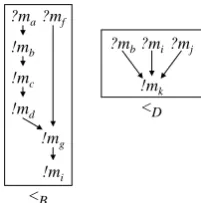
The distance between two events on a time-line does not represent any literal measurement of time, only that non-zero time has passed. Events on the same time-line are ordered linearly down the page, except where they occur within a coregion or distinct threads of a parallel con-struct. Within a coregion events are not locally ordered. Each coregion can only occur on a single time line. It is depicted by a short dashed line delineated by short horizontal lines. For process D in Figure 1, events ?mb, ?mi and ?mj are unordered as they occur within a coregion.
A parallel construct in an SD, denoted by keywordPAR, describes a set of concurrent threads that occur in the diagram. Horizontal dotted lines delineate the different threads. Hence, events from one thread are not causally ordered with respect to events from any other thread. Figure 1 contains a parallel constructs split into two threads. The first thread contains messagesma,mb,mc and md, while the second thread
contains messagesmeandmf. The bounding box of a parallel construct
has no effect on the ordering of events, it solely delineates the scope of the concurrent threads. For example, receive event !mg is ordered
with respect of one another since they are in separate threads. Events within a particular thread are ordered in the usual way, so for example, !ma must be before ?md.
The UML notation also allows a message to be split into lost and found events. This allows a message to be sent in one scenario and received in another. The send part of the message is represented by a lost event, and the receive part by a found event. In this paper we will only use this construct to simplify the visual layout of scenarios. So that the found event corresponding to a lost event always occur in the same scenario. Figure 1 gives an example where message mb has been
split into lost and found events. The lost event for !mb is depicted by
the solid circle terminating the arrow mid-process. The found event for ?mbis depicted by the empty circle that initiates an arrow into process
D. In this paper we follow the convention that the found event given by a message must always occur after the lost event for the message. The UML standard does not make any formal link between a lost event and a found event, that is it does not identify them as component parts of a single message. However, our convention is only used in simplifying the visual layout of our example and does not affect the theoretical results in any way.
2. Partial order scenarios
In this section we define the causal semantics for partial order scenar-ios. We use the same message semantics as the MSC 2000 standard [33]. Hence, a partial order scenario defines a set of message exchanges between processes with asynchronous communication channels.
DEFINITION 2.1.
− A partial order over a setE is a binary relation< such that
<is irreflexive, i.e. there is no x∈E wherex < x
<is transitive, i.e. if x < y and y < z thenx < z
<is asymmetric, i.e. there are no elementsx, y∈Esuch that x < y and y < x
− A total order over the set E is a partial order on E where for any two distinct elements aand b, eithera < b orb < a.
− Two elementsxandy ofEare unordered if¬(x < y) and¬(y < x).
We define a set to be unordered if every pair of distinct elements from that set are unordered.
Let P be a set of processes. A message m between processes is a pair (!m,?m) where !m is the send event for m, and ?m is the receive event form. LetE be the set of all send and receive events between all processes.
DEFINITION 2.2. A partial order scenario Scon processes P is
− a collection of disjoint setsE(P)⊆E, for each P ∈ P
− a set of partial orders<P, where<P is a partial order on E(P)
and is referred to as the process order forP
subject to the constraint that for each send event !m in a set E(P) the corresponding receive event ?m occurs in some set E(Q). Note it is possible forP =Q.
?ma
!mb
!mc
!md ?mf
!mg
!mi
B <
D <
?mb?mi?mj
[image:10.595.242.343.409.511.2]!mk
Figure 2. Examples of Process Orderings for Figure 1
For example, in Figure 1 all the process orders are total except for <B and <D. These process orderings are depicted as Hasse diagrams,
shown in Figure 2.
DEFINITION 2.3. The causal ordering <C on a partial order sce-nario Sc is the transitive closure of the relation given by
∪
P∈P(<P)∪
{(!e, ?e)|!e∈E(P) and ?e∈E(Q) for some P, Q∈ P}
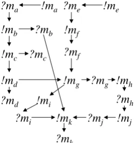
The set of pairs (!e, ?e) is used to assert that orderings between processes can only be a consequence of message exchanges. Hence, the causal ordering combines process orderings solely through the causality between send and receive event pairs. As an example, Figure 3 depicts the causal ordering for the sequence diagram in Figure 1.
Note, it is possible for there to be two events x and y, both in the same process P, where x <C y but ¬(x <P y). Without loss of
generality we will assume this is not the case from now on. That is, when x, y ∈ E(P), we assume x <C y if and only if x <P y. This
is acceptable within our context as we want to study the externally observable system behaviour and will never need to consider when the process ordering is not the same as the causal ordering. Hence, if we are given a causal ordering it will be straightforward to extract the process orderings from it.
?ma
!mb
!mc
!md
?mf
!mg ?mb
?mi !mk ?mj !ma
!mf
?mc
?md
?me !me
?mh !mh
!mi
!mj
?mk
[image:11.595.226.362.362.506.2]?mg
Figure 3. Causal Order for Figure 1
?m
a!m
b!m
c!m
d?m
f!m
g?m
b?m
i!m
k?m
j!m
a!m
f?m
c?m
d?m
e!m
e?m
h!m
h!m
i!m
j?m
k?m
gS
a
[image:12.595.180.411.73.245.2]cns(a,S,<)
Figure 4. Examples ofSandcns(a, S, <) for Figure 3
3. Causal Communication Semantics
In this section we define an elementary process algebra term P(Sc) that defines the causal behaviour of a scenario Sc up to bisimulation equivalence. In order to define P(Sc) we first have to set up some notation.
DEFINITION 3.1. For a setS⊆E and partial order<onE define
n(S, <) = {x∈E| ∃y∈S:y < x, and
¬∃z∈E: y < z < x} m(S, <) = {x∈S| ¬∃y∈S : y < x} cns(a, S, <) = m((S− {a})∪n({a}, <), <)
message mf and mc have been sent and not yet received. The events
that are eligible to occur next are given by S as shown in Figure 4. Suppose that !md occurs next in the trace. In that case ?md could
consecutively follow !mdin the trace, whereas !mgcould not. The reason
for this is that although ?md is a trigger for !mg so is ?mf, which has
not yet occurred in the trace. Hence the events that are eligible to occur consecutively with !mdare ?mc, ?mdand ?mf. That is, in this example
cns(a, S, <) = {?mc,?md,?mf}. These events are shown in Figure 4
enclosed by the dashed line.
We can now define a recursive process algebra term that defines the causal behaviour of a scenario Sc.
DEFINITION 3.2. For a setS⊆E and partial order<onE define
P(S, <) = ∑ {a∈S}
a·P(cns(a, S, <), <)
and P(∅, <) = 0. Where · denotes action prefix and ∑ denotes the usual choice operator for a process algebra term.
LetScbe a partial order scenario over processesP, with causal order <C. Define
P(Sc) =P(m(E, <C), <C)
This description is equivalent to the descriptions in [1, 11] of process algebra characterisations of the causal semantics for a partial order scenario. [21] proved (Lemma 4.5) that this particular description does indeed characterise the correct traces for Sc. That is the traces for P(Sc) are exactly the system traces of Sc(see Definition 2.4).
4. Race Conditions
A race condition represents a semantic inconsistency between the spec-ified order that events are meant to occur in and the actual order that it is possible for them to occur in. In our context ‘possible’ is interpreted within a distributed asynchronous environment. Within a partial order theoretic framework we can define a race formally as follows.
DEFINITION 4.1. Define a partial order < on E to be race free when for every eventx and message e:
x <?e⇒(x <!e or x=!e)
A B C D E F G
ma:AudioChannelReq
mb:FwdReq mc:DeviceAllocation1
md:DeviceAllocation 2
me:RouteInfoReq mf:InfoVerifyReq
mg:VerifyResponse
mh:RouteResponse mi:CallUpdate
[image:14.595.138.448.75.256.2]mj:ContinuityReq mk:ContinuityResponse
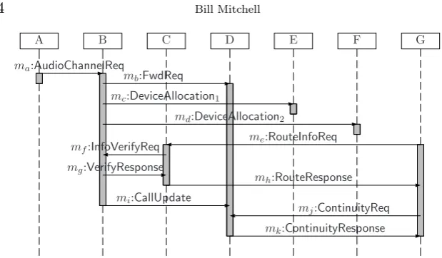
Figure 5. Motorola example containing race conditions
From this definition we see a race occurs when there is an event x and a messageesuch thatx <?eandx6<!e. That is two processes are meant to be coordinating to ensure thatxoccurs beforeeis received. In a distributed asynchronous environment that implies x occurs before !e. Otherwise !e can be sent without reference to x, and that could mean ?earrives earlier than x, contradicting the causal order. Figure 5 depicts a UML 2.0 sequence diagram taken from a Motorola proprietary case study. The study looked at approximately one hundred sequence diagrams that were part of a 3G protocol stack specification, of which fifteen contained multiple interrelated race conditions. The diagram is anonymized to protect proprietary information. In the discussion we will use the short form of message names from the sequence diagram for brevity. Altogether there are seven races in the scenario. Receive event ?mf is in a race with each of ?ma, !mb, !mc and !md. For
ex-ample, !md <C?mf but ¬(!md <C!mf). Thus process C must ensure
that mf is received after md is sent, and yet there is no coordination
between processes that can enforce this. The remaining three races occur between each of ?mb, ?mi and ?mj.
This is an interesting example in that it illustrates how multiple race conditions can be interrelated. Attempting to resolve each of the race conditions independently in a piecemeal fashion would not necessarily lead to a satisfactory solution. For example, messagemf is independent
of md (in that it can be sent at any time after ?me, and me is one of
the initial messages in the scenario). Resolving the race between ?mf
and !md by itself would not resolve the races between ?mf and ?ma,
!mb and !mc. Rather it would complicate the process of identifying a
5. Optimal Race Resolution
In this section we give a brief introduction to the inherent causal sce-nario defined in [21]. Also, we explain how the inherent causal scesce-nario defines a canonical race free generalisation for partial order scenarios.
Faced with the complex set of race conditions exemplified by Figure 5, a natural question to ask is whether there is always a non-trivial generalisation of a scenario that removes race conditions. In the partial order setting for this paper that translates into the question:
LetSc be a partial order scenario with eventsE, processes P with process orders <P for P ∈ P and causal order <C. Is there a
non-trivial partial order scenario over the same set of events and processes with a race free causal order <C0 that is a generalisation
of <C.
Partial order <1 is a generalisation of <2 if, when regarding a partial order as a set of pairs, (<1) ⊆ (<2). That is <1 has weakened some of the constraints defined by<2. This question motivated the research in [21]. [21] proved there is a unique minimal race free generalisation of a partial order scenario, which is referred to as the inherent causal scenario. In addition, [21] proves that any race free partial order sce-nario that simulates the behaviour of a partial order scesce-nario must also simulate the behaviour of its inherent causal scenario. So that the inherent causal scenario is unique up to simulation equivalence.
In order to construct the inherent causal scenario, first a particular partial order known as the inherent causal ordering is constructed. The inherent causal order is generalised from the causal order of a scenario as explained in the following definition.
DEFINITION 5.1. The inherent causal ordering<Iof<C is defined
to be the transitive closure of the following binary relation<. For every event xand message edefine:
1. x <!e ⇐⇒ x <C!e
2. !e <?e
The inherent causal scenario is the realisation of the inherent causal order in the form of a partial order scenario. The inherent causal order is race free in the sense of Definition 4.1. It is also the unique minimal generalisation of <C that is race free.
minimal race free generalisation of Figure 5. Note race conditions have been resolved by introducing additional concurrency into the original scenario. Message flows have been split into concurrent threads within a parallel construct to prevent them racing against each other. As men-tioned in the introduction, we have used the lost and found construct as a visual convenience to split mb into two parts.
The partial order given in Figure 3 is therefore the inherent causal order of Figure 5, as well as being the causal order of Figure 1. Note, although the inherent partial order scenario is unique, its graphical representation is not. Thus, Figure 1 is only one way of graphically depicting the behaviour of the inherent causal scenario as a UML sequence diagram.
Finally in this section we quote the result from [21] that formally describes how the inherent causal scenario gives a canonical race free generalisation of a partial order scenario, up to simulation equivalence.
DEFINITION 5.2. The inherent process behaviour of a partial order scenario Sc is defined to be
PI(Sc) =P(m(E, <I), <I)
Let = denote the standard simulation relation for process algebras. That is P =Q iff
for every transition Q −→a Q0, there exists a transition P −→a P0 whereP0 =Q0
PROPOSITION 5.3. [Theorem 7.2 [21]]
1. <I is race free.
2. (<I) ⊆ (<C), and PI(Sc)=Pc(Sc)
3. For any race free partial order <that preserves message ordering, let P< =P(m(E, <), <). Then P< = P(Sc) iff (<) ⊆ (<I) ⊆
(<C) andP<=PI(Sc)
That is PI(Sc) is the canonical process that simulates Pc(Sc) and is
6. Lazy Buffer Realization of Scenarios
For this section the purpose of a scenario specification is to show how processes must behave locally, rather than what global behaviour must be enforced. Rather than assume a specification scenario contains adequate coordination to ensure there are no race conditions, in this section we assume that a receiving process must determine in what order messages were actually sent, or at least in what order incoming messages should be consumed. A simple mechanism to achieve this is to provide each process with its own unbounded random access buffer, where incoming messages are stored until they are needed.
In this section we describe a modified form of the structural seman-tics given in [11] that defines our lazy buffer realization for a partial order scenario. Our goal is to construct a model where we can for-mally reason about how this buffer mechanism affects the observable global system behaviour. Hence, our model must directly describe how messages are delivered to a buffer and then consumed from the buffer. Let Sc be a partial order scenario over processesP. For P ∈ P we will define a process term Pr(P), which together with a parallel com-position operator kd, defines the lazy buffer realization for Sc (where
the subscript d denotes that kd is a distributed form of concurrent
composition).
As in [11], processes do not transmit messages directly to one an-other. Instead, there is a special transmission channel process,T, where all messages are sent. Unlike the transmission channel in [11] T will now simply transfer messages in an arbitrary fashion to simulate asyn-chronous message passing. It will be assumed that the messages are always delivered to the correct process. For convenience we assume messages have unique labels that identify which process they can be delivered to.
A process term Pr(P) is a triple Pr(In, S, <), where In is an input buffer multi-set, S is a set of concurrent events that are eligible to occur next in a trace for the process, and < is the partial order that constrains what order events occur in for that process. The distributed behaviour for a processP ∈ Pis defined to bePr(∅,m(E(P), <P), <P).
Here the input buffer is initialised as empty, the initial set of events are the minimal events inP with respect to the process order forP, and of course the process order forP defines how trace events are constrained. The buffer mechanism splits the act of receiving a message into message delivery followed later by message consumption.
Receive φ=Pr(In, S, <P) φ−→?e Pr(In∪ {?e}, S, <P)
?e∈E(P)
Consume φ=Pr(In∪ {?e}, S∪ {?e}, <P) φ−→τ Pr(In,cns(?e, S, <P), <P)
Send φ=Pr(In, S∪ {!e}, <P) φ−→!e Pr(In,cns(!e, S, <P), <P)
!e6∈S
Transmit φ
!e −→φ0
T(B)kdφ−→!e T(B∪ {?e})kdφ0
Deliver φ
?e −→φ0
T(B∪ {?e})kdφ−→?e T(B)kdφ0
[image:18.595.125.395.74.330.2]Terminate Pr({ },{ }, <P) =End(P)
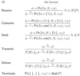
Figure 6. Lazy Buffer Realization Semantics for Partial Order Scenario
for each P ∈ P. This term can not perform any action and represents a parameterised version of the 0 process.
DEFINITION 6.1. Let τ denote the silent action. Define the dis-tributed composition operator kd to have the operational semantics
given in Figure 6. Further, kd is defined to be associative and
commu-tative. For eachP ∈ P, define
Pr(P) =Pr(∅,m(E(P), <P), <P)
Define the lazy buffer realization of Scto be
Pd(Sc) =T(∅)kdPr(P0)kd· · · kdPr(Pn)
Notice that in Definition 6.1 we only define kd for composition
The Receive rule states that a process can accept any receive event at any point during execution, as long as the event belongs to that process. A process initially places any received event into its input buffer. Suppose that the process term for P is Pr(In, S, <P) at some
point during its execution. The setSdefines concurrent events that are eligible to occur next in the execution of P. The Send rule allows an event !eto be sent byPwhenever !eis one of the events inSirrespective of what events are in buffer In.
The Consume rule states that an event ?e can be taken from the input buffer In if and only if that is also an element of S. That is an event can only be consumed from the input buffer when that event is one of the concurrent events that is eligible to occur next according to the process order forP. SinceInis a multiset the order that events are consumed from it are solely determined bySand<P. We have modelled
message consumption as an internal action by using τ to describe the external action that will be observed when messages are consumed. The Consume rule is the only rule that defines an interaction between S and In. It is the Consume rule that defines how processes adopt a lazy approach to internally consuming message events.
The Transmit rule states that whenever a send event !eis executed by a process then T will store the corresponding receive event ?e in the transmission buffer B. The Deliver rule states that T can remove an event from its buffer and place it in the input buffer of a process whenever that process is able to accept such an event. Since the Receive rule allows a process to accept a receive event at any time this implies T can deliver messages in an arbitrary manner.
Note that once an event a occurs (and is consumed in the case of a receive event) then cns(a, S, <P) defines the set of events that can
be consecutive to a in a trace of P. This is analogous to the causal semantics given in Definition 3.2. Hence, the setS will always contain concurrent events that are consistent with<C.
Each of the Pr(P) processes locally realizes the causal order <C in the sense that messages can only be consumed in the order given by <P, as opposed to attempting to enforce the causal order <C. Also a
message !e is sent only when the correct stimuli have been consumed in the correct order from the input buffer.
buffer realization can not deadlock. This demonstrates that our seman-tics enables processes to continue to act and consume messages with respect to the local process ordering even when events are not delivered correctly at the global level.
DEFINITION 6.2. Let Scbe a partial order scenario over processes Pi for 1≤i≤n. LetEndi =End(Pi). Write Q0
α
−−−→?Qm, where α=
a1·a2· · ·am, when there are processesQi and transitions Qi ai −→Qi+1 for 0≤i≤m−1.
Define a sequence of events β =b1·b2· · ·bk to be a deadlock trace
for Pd(Sc), if there exists a process Q 6= End0 kd · · · kd Endn where
Pc(Sc) β
−−−→? T(B) kd Q, for some buffer B, and T(B) kd Q can not
perform any action according to the rules in Figure 6.
PROPOSITION 6.3. Let Sc be a partial order scenario over pro-cesses Pi for 1≤i≤n.
Pd(Sc) has no deadlock traces.
Proof
Suppose there is a partial trace β = b1· · ·bk of Pd(Sc). Then we
can suppose there are terms φk
i =Pr(Inki, Sik, <Pi), and
ψk=T(Bk)kdφk0 kd· · · kdφkn where
Pd(Sc) β −−−→?ψk
That is eachφki is the process thatPi has become oncePd(Sc) has
transformed into ψk. Bk contains the events that are still to be
delivered at the end of the trace. Let ER denote the set of receive
events in the set of all events E.
AlthoughT(B) is constrained by the operational semantics of Def-inition 6.1 it can always deliver any messages remaining inB. Also, any process φki can send a message to T so long as there is some send event inSk
i. Thus a deadlock can occur if and only ifBk=∅
and
∀0≤i≤n.(Sik⊆ER) and (Sik∩Inki =∅)
Let
?e∈m( ∪ 0≤i≤n
and suppose that ?e∈Sikfor somei, and that !e∈E(Pj) for some
j. If !e has not already occurred in β this can only be because there is some x ∈ Sjk where x <Pj!e. This contradicts that ?e is
minimal. Hence, !e=br for some 1≤r≤k. SinceBk=∅this can
only be true if ?e∈Inki, which is a contradiction. This completes
the proof. 2
DEFINITION 6.4. For a set of events X, let !X be the set of all send events contained in X, and let ?X be the set of all receive events inX. Given a termPd0 of the form
T(B0)kdPr(P1)0 kd· · · kdPr(Pn)0
wherePr(Pi)0 =Pr(Ini0, Si0, <Pi) for 1≤i≤n, let
S(Pd0) =B0∪ ∪ 1≤i≤n
!Si0
This set will be used later in the proof of the main result of the paper Proposition 6.5.
When Pd0 represents the system state at some point, then S(Pd0) rep-resents the set of send events in all the system processes and all the receive events in the transmission buffer that are eligible to occur next. We can now state and prove the main result of the paper. The globally observable behaviour defined by the lazy buffer realization for Sc is weak bisimulation equivalent to the global behaviour defined by the inherent causal scenario forSc.
PROPOSITION 6.5. Let Sc be a partial order scenario, and let ' denote weak bisimulation equivalence. Then
PI(Sc)'Pd(Sc)
Recall that the process term PI(Sc) on the left is defined in terms
of the causal semantics of Definition 3.2. PI(Sc) = P(m(E, <I), <I),
which defines the globally observable behaviour of the inherent causal scenario.
Proof
Let Scbe a partial order scenario over processes
P ={Pi |1≤i≤n}. So we may write
LetPd=Pd(Sc) and let
PI =P(m(E, <I), <I)
To prove weak bisimulation equivalence we prove the following stronger result. Let α =a0· · ·ak be a sequence of events fromE.
We will prove there exists
Pd0 =T(B0)kdPr(P1)0kd· · · kdPr(Pn)0
wherePr(Pi)0=Pr(Ini0, Si0, <Pi) for 1≤i≤nand
Pd α −−−→?Pd0
if and only if there exists some
PI0 =P(S0, <I)
whereS0 ⊆E such that PI α
−−−→? PI0 and where
S(Pd0) =S0
See Definition 6.4 for the definition of S(Pd0). Once all the events in α have occurred, the set S(Pd0) represents all the send events that are permitted to concurrently occur next in each process inSc and all the current receive events in the buffer for the transmission channel. A corollary of the proof hypothesis is that Pd(Sc) andPI
can always perform the same traces, and at every point during the execution of a trace they contain exactly the same events that are eligible to concurrently occur next. We are not interested in process receive events as they are consumed internally, only receive events delivered from the transmission buffer will be externally observable.
Induction statement
This stronger statement can be proved by induction on the length of α. The base case where the length ofα = 0 is trivial so we can move on to the induction step.
Case a=!e
Consider first where a=!e, and supposePd0 −→!e Pd00. Let
PI00=P(S00, <I)
whereS00=cns(!e, S0, <I). To proveS00=S(Pd00) we will show that
?S00=?S(Pd00) and !S00=!S(Pd00), which we will prove in that order.
By the induction hypothesis we may suppose that !e∈Sr0 for some r. LetSr0 ={!e} ∪Sr00. We can then writePd0 in the form
Pd0 =T(B0)kdPr(Inr0,{!e} ∪Sr00, <Pr)kdQ
where Q is just a place holder to collect together all the other Pr(Pi)0 terms. Therefore there is a transition
Pd0 −→!e
T(B0∪ {?e})kdPr(In0r,cns(!e, Sr0, <Pr), <Pr)kdQ
LetB00=B0∪{?e}, and (<r) = (<Pr). From the definition for<I
it is immediate that ?e∈ cns(!e, S0, <I), since all of the elements
inS0−{!e}are disjoint from !ewith respect to<I. This means the
only new receive event in S00 that was not already present in S0 is ?e. Hence, B00 is the set of receive events for S00, which implies ?S00=?S(Pd00).
It remains to prove that !S00 =!S(Pd00). We first prove that !S00 ⊆ !S(Pd00). We need to consider what new send events are present in S00 that are not elements ofS0. It will be enough to prove that for any new send event !g∈S00then !g∈cns(!e, Sr0, <r). By inspection
any new send events in S00 must come from the set n(!e, <I).
From the definition of the causal ordering <C it follows that
n(!e, <I)⊆ {?e} ∪ {x∈E(Pr)|!e <Cx}
Consider the case where ?g ∈ n(!e, <I). By definition that means
!e <I ?g, and there is no x such that !e <I x <I ?g. From the
definition of <I that can only hold if ?g=?e. If this were not the
case then the inequality could only hold if !e <I ?e <C !g <I ?g,
which contradicts that ?g∈n(!e, <I). Therefore,n(!e, <I) consists
of only one receive event ?eplus some number of send events. Since ?e∈cns(!e, S0, <I), we knowcns(!e, S0, <I)−S0 consists of ?eplus
a number of send events.
Consider when !g ∈ n(!e, <I). Then ¬(?e <C !g), for otherwise
!g 6∈ n(!e, <I). Therefore, we have !e <r !g. Further there is no
That is any new send event in S00 that is not already in S0 must actually be an element ofn(!e, <r).
A new send event !ginS00must also be an element ofcns(!e, S0, <I).
Note, any such !gis also minimal inS0− {!e} with respect to<I.
Let !g be a new send event in S00, so that !g ∈ cns(!e, S0, <I) ⊆
n(!e, <I), and hence !g ∈ n(!e, <r). To complete the proof that
!S00 ⊆ !S(Pd00) we only need to prove that !g is also minimal in S0 − {!e} with respect to <r, since that will complete the proof
that !g∈cns(!e, Sr0, <r).
For a contradiction, consider if there is some elementy∈Sr0 where y <r!g, andy 6=!e. We knowy is not a send event. If this were not
the case, theny ∈!Sr0 ⊆S0. That would imply !g6∈cns(!e, S0, <I),
which is a contradiction. Therefore, we may assumey=?ffor some f. Since ?f ∈ E(Pr) this event has not yet occurred. Therefore
there is some eventz <C?f, where
z∈B0∪ ∪
j6=r
Sj0
Hence,z <I !g,z∈S0 and zis distinct from !e. Therefore we have
a contradiction since this again implies !g 6∈ cns(!e, S0, <I). This
proves that !g∈cns(!e, Sr0, <r). Hence, in the case where a=!ewe
have shown that
!S00⊆S(Pd00)
The proof that !Sr00 ⊆ S00 is analogous so that we have proved S00 = S(Pd00). This completes the proof of the induction step for the case a=!e.
Case a=?e
Consider next the case wherea=?efor some messagee. We follow the same pattern as for the previous case in that we prove the receive events for S00 andS(Pd00) are the same, and then that their send events are the same. We may write Pd00 in the form
Pd00=T(B00)kdPr(P1)00kd· · · kdPr(Pn)00
where Pr(Pi)00=Pr(In00i, Si00, <Pi).
From the definition for<I it follows that forx∈E, ?e <I xif and
only if one of the two conditions below hold
• There is some g∈E such thatx=!g and ?e <C!g
• There is some g∈E such thatx=!g and
Note the second item is true if and only if ?e <I !g <C ?g.
Whichever case applies, it follows that every element of n(?e, <I)
is a send event in E.
The induction hypothesis implies that ?e ∈ B0, and hence there is a transition PI0 −→?e PI00. We can also assume without loss of generality that ?e is consumed from the relevant input buffer at this point, if that is permitted by the process order. Hence, we have proved that the receive events inS00 are exactly the events in B00=B0− {?e}, which implies that ?S00=?S(Pd00).
What remains to be proved is that !S00=!S(Pd00). To prove that it is enough to prove the send events inS00are the union of all the !Si00. First we prove that !Sj00 =!cns(?e, Sj0, <C) ⊆cns(?e, S0, <I), where
?e∈E(Pj).
Let !g ∈ n(?e, <j), which implies ?e <j !g, and hence ?e <I !g.
Also notice that
∀x∈E(Pj).¬(?e <j x <j !g)
Given that we knowu <I v⇒u <C v we can prove
∀x∈E(Pj).¬(?e <Ix <I !g)
To prove this, assume for a contradiction that there is some x ∈ E−E(Pj) where
?e <I x <I !g
This implies ?e <C x <C!g since (<I) ⊆ (<C). However, it then
follows that there is some ?h ∈ E(Pj) such that x <C?h <j !g.
Therefore, ?e <C ?h <j !g, which implies ?e <j ?h <j !g and we
have a contradiction as required.
Thus, we have proved !g ∈ n(?e, <I). A similar argument also
shows that
!g∈cns(?e, S0, <I)
Hence,
!cns(?e, Sj0, <C)⊆cns(?e, S0, <I)
and so we have proved that !Sj00 ⊆ S00. Since none of the other processes have changed during this transition it is still true that for i 6= j, !Si0 ⊆ S00. The converse, that !S00 is contained in the union of all the !S00i for 1 ≤ i ≤ n, is analogous and so we omit the details. This completes the proof that !S00=!S(Pd00), and so we have provedS00=S(Pd00).
2
As an illustration of Proposition 6.5, we can return to Figures 5 and 1. If the scenario in Figure 5 is realized according to the lazy buffer semantics of Definition 6.1, then the behaviour that would be externally observable is that shown in Figure 1. ProcessD, for example, is specified in Figure 5 to realize a total order on its events. However, this behaviour can not be realized within a distributed asynchronous environment. The actual behaviour that would be observed is given by the process partial order forDin Figure 2. As we can see from Figure 2, in a distributed environment this linear specification would be locally realized as three independent receive events followed by a final send event.
7. Conclusion
Practitioners use scenario specification languages like UML or MSC to rapidly develop requirements specifications. Frequently they use these languages in a semi-formal manner. Scenarios sometimes tend towards specific examples that contain domain specific assumptions instead of defining exemplary generalisations. This can lead to specifications that are semantically inconsistent at the global level of process coordination. Such discrepancies can result in race conditions.
The inherent causal scenario and lazy buffer realization defined in the paper represent two orthogonal views of how race conditions may be resolved. The inherent causal scenario generalises a specification by just enough to remove race conditions. Thus, the inherent causal scenario generalises a specification to ensure that the actual observed global behaviour will match the specified behaviour. However, the inherent causal ordering is difficult to relate to standard software engineering constructs, which can make it difficult for practitioners to accept.
a straightforward communication semantics and it is intuitively clear why it correctly resolves race conditions. From anecdotal evidence, this seems to be a commonly used realization of a sequence diagram.
The paper has proved these two apparently different approaches are, at the globally observable level, the same. Hence, realizing a sce-nario with lazy buffers defines the unique minimal generalisation of the scenario to remove all race conditions. Since the inherent causal scenario is itself a partial order scenario, we have also proved that the lazy buffer realization is equivalent to a partial order scenario. This demonstrates that the lazy buffer realization does represent a coherent semantic solution to race avoidance. Therefore, in this particular sense, the lazy buffer pragmatic approach is the theoretically best possible solution to resolving race conditions. The proof is an equivalence and so we have also proved that the inherent causal scenario is a genuine ‘real-world’ software engineering solution to resolving race conditions.
References
1. Alur, R. and Yannakakis, M. 1999, Model checking of message sequence charts, Proceedings of the Tenth International Conference on Concurrency Theory, LNCS 1661, Springer, pp 114–129.
2. Alur, R. and Etessami, K. and Yannakakis, M. 2000, Inference of Message Sequence Charts, Proceedings 22nd International Conference on Software Engineering, pp 304-313.
3. Alur, R. and Etessami, K. and Yannakakis, M.2001, Realizability and verification of MSC graphs, Proceedings of the 28th International Colloquium on Automata, Languages, and Programming, Springer, New York, pp 797-808.
4. Ben-Abdhallah, H. and Leue, S. 1997, Syntactic detection of process divergence and non-local choice in message sequence charts, Proceedings of the 3rd International Conference on Tools and Algorithms for the
Construction and Analysis of Systems, Springer, pp 259-274.
5. Baker, P. and Bristow, P. and Jervis, C. and King, D. and Mitchell, B. 2002, Automatic Generation of Conformance Tests From Message Sequence Charts, Proceedings of 3rd SAM Workshop, Telecommunications and Beyond: The Broader Applicability of MSC and SDL, LNCS 2599, Springer, pp 170-198. 6. Beyer, M. and Dulz, W. and Zhen, F. 2003, Automated TTCN-3 Test Case
Generation by Means of UML Sequence Diagrams and Markov Chains, Proceedings of 12th Asian Test Symposium (ATS’03), IEEE, pp 102–106. 7. Bontemps, Y. and Schobbens, P. 2003, Synthesis of Open Reactive Systems
from Scenario-Based Specifications, Third International Conference on Application of Concurrency to System Design (ACSD’03), IEEE, pp 41-50. 8. Bontemps, Y. and Heymens, P. 2002, Turning high-level live sequence charts
9. Chung, S. and Kim, H. S. and Seop Bae, H. and Kwon, Y. R. and Lee, B. S. 1999, Proceedings International Symposium on Software Engineering for Parallel and Distributed Systems, pp 72 – 82.
10. Clarke, E. and Andwing, J. 1996, Formal methods: State of the art and future directions. ACM Computing Surv., 4(28), pp 626–643.
11. Gehrke, T. and Hilhn, M. and Wehrkeim, H. 1998, An Algebraic Semantics for Message Sequence Chart Documents, in Proceedings of the FIP TC6 WG6.1 Joint International Conference on Formal Description Techniques for Distributed Systems and Communication Protocols (FORTE XI) and Protocol Specification, Testing and Verification (PSTV XVIII), pp 3–18. 12. Gunter, E. and Muscholl, A. and Peled, D. 2003, Compositional Message
Sequence Charts, International Journal on Software Tools for Technology Transfer (STTT), Springer, 5(1), pp 78–89.
13. Holzmann, G. J. and Peled, D. A. Message Sequence Chart Analyzer, United States Patent, 5,812,145.
14. Holzmann, G. J. and Peled, D. A. and Redberg, M. H. 1996, An Analyzer for Message Sequence Charts, Software Concepts and Tools, 17(2), pp 70–77. 15. Harel, D. and Damm W. 2001, LSCs: Breathing Life into Message Sequence
Charts, Formal Methods in System Design, 19, pp 45–80.
16. Harel, D. and Kugler, H. 2002, Synthesizing state-based object systems from LSC specifications, International Journal of Foundations of Computer Science, 13(1), pp 5–51.
17. Leue, S. and Mehrmann, L. and Rezai, M. 1998, Synthesizing Software Architecture Descriptions from Message Sequence Chart Specifications, Proceedings 13th IEEE International Conference on Automated Software Engineering, IEEE, pp 192–195.
18. Lohrey, M. 2002, Safe Realizability of High-level Message Charts. In Proceedings of the 13th International Conference on Concurrency Theory (CONCUR).
19. Mauw, S. and Reniers, M. A. 1995, An Algebraic Semantics of Basic Message Sequence Charts, The Computer Journal, 7(5), pp 473–509.
20. Mauw, S. and Reniers, M. A. 1999, Operational Semantics for MSC’96 Computer Networks, 31(17), 1785–1799.
21. Mitchell, B. 2005, Resolving Race Conditions in Asynchronous Partial Order Scenarios, IEEE Transactions on Software Engineering, 31(9), pp 767- 784, preliminary version also appeared as [22].
22. Mitchell, B. 2004, Inherent Causal Orderings of Partial Order Scenarios, International Colloquium on Theoretical Aspects of Computing, Guiyang China, LNCS 3407, Springer, pp 114–129.
23. Mitchell, B. and Thomson, R. and Jervis, C. 2003, Phase Automaton for Requirements Scenarios, Proceedings of Feature Interactions in
Telecommunications and Software Systems VII, IOS Press, pp 77-84. 24. Object Management Group. Unified Modelling Language Specification,
Version 2.0 Specification, OMG, 2004. http://cgi.omg.org/.
25. Peled D. 2002, Specification and Verification using Message Sequence Charts. Electronic Notes in Theoretical Computer Science, 65(7).
26. Rudolph, E. and Schieferdecker, I. and Grabowski J. 2000, Development of a MSC/UML Test Format, Formale Beschreibungstechniken fur verteilte Systeme, Verlag Shaker, pp 153-164.
International Symposium of Formal Methods Europe, LNCS 3582, Springer, pp 415-431.
28. Schumann, J. and Whittle, J. 2000, Generating Statechart Designs From Scenarios, Proceedings of the 22nd international conference on Software engineering, pp 314–323.
29. Wang, H. H. and Qin, S. and Sun, J. and Song Dong, J. 2007, Realizing Live Sequence Charts in SystemVerilog, Proceedings of First Joint IEEE/IFIP Symposium on Theoretical Aspects of Software Engineering, TASE, IEEE, pp 379-388.
30. Whittle, J. and Saboo, J. and Kwan, R. 2005, From Scenarios to Code: an Air Traffic Control Case Study, Journal of Software and Systems Modeling, Springer, 4(1), pp 71–93.
31. Tsiolakis, A. 2001, Integrating Model Information in UML Sequence Diagrams, Electronic Notes in Theoretical Computer Science, 50(3), pp 266–274.
32. Uchitel, S. and Kramer, J. and Magee, J. 2004, Incremental Elaboration of Scenario-based Specifications and Behaviour Models using Implied Scenarios, ACM Transactions on Software Engineering and Methodology (TOSEM), 13(1), pp 37—85.