Chapter 7
3
×
CO
2
stabilisation experiments
7.1
Introduction
The ability of the Mk3L coupled model to simulate the climate of the mid-Holocene was evaluated in Chapter 6. In this chapter, the transient response of the model to an increase in the atmospheric carbon dioxide concentration is investigated. A scenario is employed in which the CO2 concentration is stabilised at three times the
pre-industrial level.
Three transient climate change simulations are presented. These are designated 3CO2-DEF, 3CO2-SHF and 3CO2-EFF; they are initialised from the states of the control runs CON-DEF, CON-SHF and CON-EFF, respectively, at the end of year 100, and are integrated to years 1400, 1100 and 1100. The transient simulations differ from the equivalent control runs only in that the atmospheric carbon dioxide concentration is increased at 1% per year. A concentration of 560 ppm (twice the pre-industrial value of 280 ppm) is reached in year 170, and a concentration of 840 ppm (three times the pre-industrial value) is reached in year 211. The CO2
concentration is held contant at 840 ppm thereafter. Further details regarding the experimental design are provided in Appendix A.
The scenario employed here differs from that of Bi et al. (2001, 2002) and Bi
(2002), who study the response of the CSIRO Mk2 coupled model to an increase in the atmospheric carbon dioxide concentration. While they also stabilise the CO2
concentration at three times the pre-industrial value, it is increased in accordance with the IS92a emission scenario (Houghton et al., 1994); a trebling of the CO2
concentration is therefore only achieved after 202 years. The scenario employed herein imposes a 1% per year increase, however, as it allows a direct comparison with the models which participated in the Coupled Model Intercomparison Project (e.g. Covey et al., 2003).
Run 3CO2-DEF is analysed in Section 7.2, indicating the response of the default configuration of the Mk3L coupled model to an increase in the atmospheric carbon dioxide concentration. Section 7.3 contrasts runs 3CO2-SHF and 3CO2-EFF with run 3CO2-DEF, assessing the impact of the ocean model spin-up procedure upon the model response.
232 CHAPTER 7. 3×CO2 STABILISATION EXPERIMENTS
7.2
The default model response
7.2.1 Atmosphere
Surface air temperature
The evolution of the simulated global-mean and zonal-mean surface air temperature (SAT) during run 3CO2-DEF are shown in Figure 7.1. Dashed vertical lines indicate year 100, being the year after which the atmospheric CO2 concentration begins to
increase, and year 211, being the year in which the concentration reaches 840 ppm. The global-mean SAT increases rapidly as the CO2 concentration increases, with
warming of 1.6◦C upon a doubling of the CO2 concentration, and 2.7◦C upon a
trebling. [These figures represent the average SAT changes for years 155–184 and 196–225 respectively, being the 30-year periods centred on the points at which the CO2 concentration reaches two and three times the pre-industrial concentration.]
The global-mean SAT continues increasing once the CO2 concentration has
sta-bilised, although at a reduced rate. By the final century of the run (i.e. years 1301–1400), the global-mean SAT has increased by 5.3◦C relative to the control
run, and is continuing to increase at a rate of ∼0.08◦C/century. The mean SAT
changes are greater over land than over the ocean, with increases of 6.2◦C and 4.8◦C,
respectively, by the final century.
Figure 7.2 shows the changes in SAT by years 1301–1400. The strongest warming occurs over the high-latitude oceans, with increases in annual-mean SAT as large as 19.4◦C in the Northern Hemisphere, and 15.6◦C in the Southern Hemisphere.
Figures 7.2b and 7.2c show that the warming at high latitudes occurs primarily in winter, with relatively little change in the summer temperatures. This is explained by the lack of insolation at high latitudes in winter, as a result of which the surface temperature is governed by the re-radiation of longwave radiation, and by the sur-face heat capacity. The increase in the atmospheric CO2 concentration leads to a
reduction in the outgoing longwave radiation, while a reduction in the sea ice cover - which has a strong insulating effect - increases the effective surface heat capac-ity. Both these changes result in higher winter surface air temperatures over the high-latitude oceans.
The climate sensitivity of the Mk3L coupled model, as indicated by the increase of 1.6◦C in the global-mean SAT upon a doubling of the CO2 concentration, is
con-sistent with those models which participated in the Coupled Model Intercomparison Project (CMIP, e.g.Raper et al., 2002;Covey et al., 2003). However, the long-term response of the model to a trebling of the CO2 concentration is ∼20% weaker than
that of the CSIRO Mk2 coupled model (Hirst, 1999; Bi, 2002).
Sea ice
Figure 7.3 shows the evolution of the sea ice extent and volume in each hemisphere during runs CON-DEF and 3CO2-DEF. There is a rapid decline in sea ice cover as the atmospheric CO2 concentration increases. Upon a doubling of the atmospheric
CO2concentration, the annual-mean sea ice extents have decreased by 2.5×10 12
m2
7.2. THE DEFAULT MODEL RESPONSE 233
Figure 7.1: The change in annual-mean surface air temperature (◦C) during run
234 CHAPTER 7. 3×CO2 STABILISATION EXPERIMENTS
Figure 7.2: The average surface air temperature (◦C) for years 1301–1400 of run
7.2. THE DEFAULT MODEL RESPONSE 235
CMIP (Flato and Participating CMIP Modelling Groups, 2004).
The decline in sea ice cover continues once the CO2 concentration is stabilised.
By the final century of run 3CO2-DEF, sea ice has almost disappeared in the South-ern Hemisphere; the average sea ice extent and volume are reduced by 90% and 92%, respectively, relative to the control run. There is also a sharp reduction in the sea ice cover in the Northern Hemisphere, with the average sea ice extent and volume reduced by 64% and 83%, respectively. Bi (2002), using the CSIRO Mk2 coupled model, finds larger changes during a similar 1400-year simulation, with the sea ice disappearing completely in the Northern Hemisphere; this behaviour is consistent with the greater warming exhibited by this model.
Figures 7.4 and 7.5 show the average sea ice concentrations and thicknesses, respectively, for the final century of the run; Figures 5.4 and 5.5 show equivalent values for run CON-DEF. The extent to which the sea ice has disappeared in each hemisphere is apparent, with summer ice cover confined to the western Ross Sea in the Southern Hemisphere, and to the central Arctic Ocean in the Northern Hemi-sphere. That sea ice which does form is thinner than in the control run, typically by
∼50% in the Northern Hemisphere, and by∼20% in the Southern Hemisphere; this accounts for the fact that the sea ice volumes in each hemisphere exhibit a larger fractional decline than the extents.
7.2.2 Ocean
Sea surface temperature and salinity
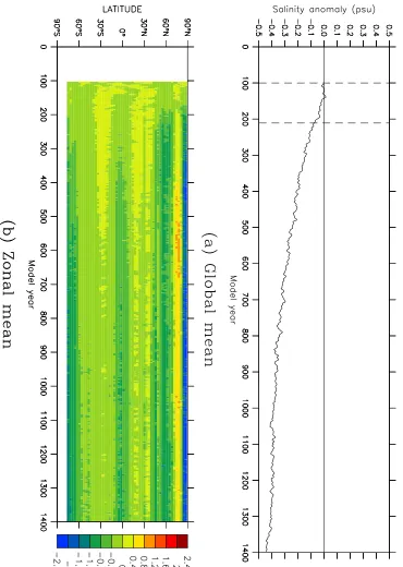
The evolution of the simulated global-mean and zonal-mean sea surface temperature (SST) and sea surface salinity (SSS) during run 3CO2-DEF are shown in Figures 7.6 and 7.7 respectively. As with the surface air temperature, the global-mean SST increases rapidly as the atmospheric CO2 concentration increases, with warming of
1.0◦C upon a doubling of the CO2 concentration, and 1.9◦C upon a trebling. The
global-mean SST continues to increase, albeit at a decreasing rate, once the CO2
concentration is stabilised. By the final century of the run, the global-mean SST has increased by 4.1◦C relative to the control run, and is continuing to increase at
a rate of ∼0.07◦C/century. The zonal-mean SST exhibits the strongest warming at
∼60◦S and∼60◦N, but there is also strong warming over the tropics.
In contrast to the surface air temperature and sea surface temperature, the global-mean SSS exhibits relatively little change as the atmospheric CO2
concen-tration increases. However, it exhibits a steady downward trend over the following centuries, before gradually beginning to stabilise. By the final century of the run, the global-mean SSS has decreased by 0.42 psu relative to the control run. The zonal-mean SSS exhibits a slight freshening at most latitudes; however, there is strong freshening at the North Pole, and an increase in the zonal-mean SSS at ∼75◦N.
236 CHAPTER 7. 3×CO2 STABILISATION EXPERIMENTS
7.2. THE DEFAULT MODEL RESPONSE 237
238 CHAPTER 7. 3×CO2 STABILISATION EXPERIMENTS
7.2. THE DEFAULT MODEL RESPONSE 239
Figure 7.6: The change in annual-mean sea surface temperature (◦C) during run
240 CHAPTER 7. 3×CO2 STABILISATION EXPERIMENTS
7.2. THE DEFAULT MODEL RESPONSE 241
surface temperatures, the SST increases are relatively uniform throughout the year. This is in contrast to the surface air temperature, where there is a much larger temperature increase in winter than during summer.
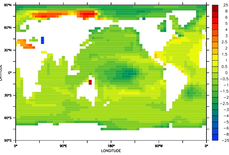
Figure 7.9 shows the change in the annual-mean SSS by the final century of the run. The isolation of the Caspian Sea from the world ocean is revealed by a decrease of 20.4 psu in the mean SSS relative to the control run. This arises from an increase of 6.7 psu in the mean SSS during run CON-DEF, and a decrease of 13.7 psu during run 3CO2-DEF. Of the remainder of the inland seas, there is a considerable increase in the salinity of the Mediterranean Sea. The Arafura Sea, between Australia and Indonesia, also experiences an increase of 6.7 psu in the mean SSS. While not an inland sea, it represents an embayment on the Mk3L ocean model grid, and is too small to contain any horizontal velocity gridpoints. The model can therefore only represent the diffusive component of the exchange of water properties with the world ocean, with the advective component being neglected.
At high latitudes, the SSS increases over the eastern Arctic Ocean, in the region where the sea ice cover has disappeared, but there is a freshening in those regions where sea ice cover persists. Over the remainder of the ocean, there is a slight salinity increase across much of the Atlantic Ocean, and a slight freshening across much of the Pacific Ocean.
Water properties
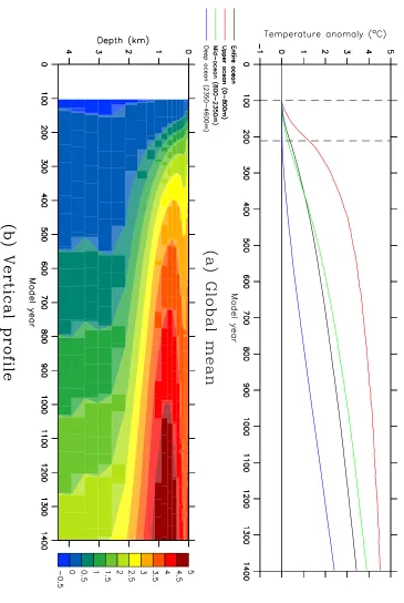
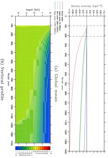
The evolution of the simulated global-mean potential temperature, salinity and po-tential density of the world ocean, and of the simulated global-mean vertical profiles, during run 3CO2-DEF are shown in Figures 7.10, 7.11 and 7.12 respectively.
The temperature of the ocean increases steadily throughout the run, warming 3.43◦C, relative to the control run, by year 1400. Consistent with the changes in
surface air temperature, the upper ocean warms rapidly as the atmospheric CO2
concentration increases. It continues to warm, but at a decreasing rate, once the CO2 concentration is stabilised; by year 1400, the temperature of the upper ocean
has increased by 4.52◦C, and it is continuing to warm at a rate of∼0.07◦C/century.
While the upper ocean exhibits the greatest warming, the temperatures of the mid-and deep oceans are still increasing rapidly by the end of the run, increasing at rates of∼0.18◦C/century and∼0.22◦C/century respectively. Thus, while the largest
global-mean temperature increase of 4.85◦C occurs at a depth of 710 m, it can be
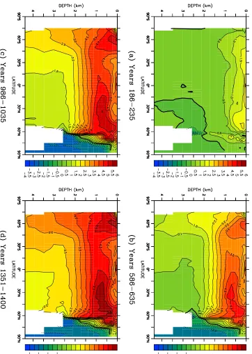
expected that the warming of the world ocean will ultimately become more uniform. The evolution of the zonal-mean potential temperature during run 3CO2-DEF is shown in Figure 7.13. Average values are shown for years 186–235, representing the 50-year period centred on the point at which the atmospheric CO2 concentration is
stabilised, for years 586–635 and 986–1035, and for the final 50 years of the run. The largest temperature increases occur in the upper ocean, at∼60◦S and∼40◦N. These
warmings propagate horizontally throughout the ocean, and can be attributed to increases in the temperatures of Antarctic Intermediate Water and North Atlantic Deep Water, arising from the surface warming.
North of 30◦S, the contours are horizontal throughout the mid-ocean, indicating
sur-242 CHAPTER 7. 3×CO2 STABILISATION EXPERIMENTS
Figure 7.8: The average sea surface temperature (◦C) for years 1301–1400 of run
7.2. THE DEFAULT MODEL RESPONSE 243
Figure 7.9: The annual-mean sea surface salinity (psu) for years 1301–1400 of run 3CO2-DEF, expressed as an anomaly relative to the annual-mean sea surface salinity for years 1301–1400 of control run CON-DEF.
face warming to penetrate slowly to depth (see below). This convection represents the only ventilation of the abyssal ocean, with the most rapid warming therefore occurring in the deep Southern Ocean. In contrast to the remainder of the world ocean, the deep Arctic Ocean cools during the first thousand years of the run; how-ever, this trend appears to reverse thereafter.
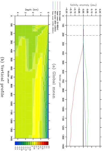
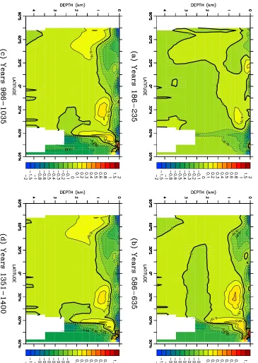
The mean salinity of the ocean decreases by just 0.004 psu, relative to the control run, during the 1300 years of run 3CO2-DEF. This is in contrast to the freshening of ∼0.1 psu encountered by Bi (2002) during a similar simulation, and indicates that the modifications to the coupling between the atmosphere and ocean models in Mk3L (Phipps, 2006) are successful at ensuring the conservation of freshwater. The surface freshening identified above, with the global-mean SSS decreasing by 0.42 psu by the end of the run, therefore represents a vertical redistribution of salt, with the surface freshening balanced by a slight increase in the salinity of the mid- and deep ocean. The evolution of the zonal-mean salinity during run 3CO2-DEF is shown in Figure 7.14. Apart from a freshening of the surface layers and of the Arctic Ocean, the zonal-mean SSS is generally stable throughout the run.
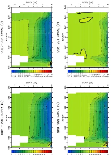
Reflecting the warming of the ocean, the mean potential density declines by 0.43 kgm−3
244 CHAPTER 7. 3×CO2 STABILISATION EXPERIMENTS
Figure 7.10: The change in annual-mean potential temperature (◦C) during run
7.2. THE DEFAULT MODEL RESPONSE 245
246 CHAPTER 7. 3×CO2 STABILISATION EXPERIMENTS
Figure 7.12: The change in annual-mean σθ (kgm−3
7.2. THE DEFAULT MODEL RESPONSE 247
Figure 7.13: The evolution of the zonal-mean potential temperature (◦C) during
248 CHAPTER 7. 3×CO2 STABILISATION EXPERIMENTS
7.2. THE DEFAULT MODEL RESPONSE 249
Figure 7.15: The evolution of the zonal-mean σθ (kgm−3
250 CHAPTER 7. 3×CO2 STABILISATION EXPERIMENTS
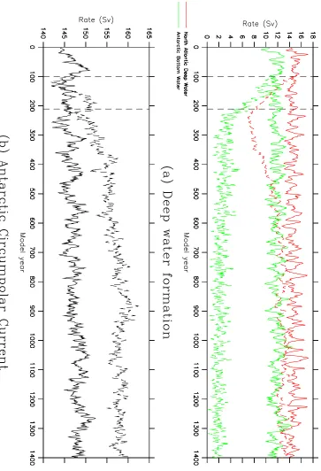
Circulation
Figure 7.16 shows the evolution in the rates of North Atlantic Deep Water (NADW) and Antarctic Bottom Water (AABW) formation, and in the rate of volume trans-port through Drake Passage, during runs CON-DEF and 3CO2-DEF. The rate of NADW formation weakens significantly as the atmospheric CO2 concentration
in-creases, with the average rate for years 211–260 being 7.5 Sv; this is 49% weaker than the average rate of NADW formation for the equivalent period of the control run.
The weakening of the thermohaline circulation in response to an increase in the atmospheric CO2 concentration is a common feature of coupled models, and has
been widely studied (e.g. Manabe and Stouffer, 1994; Stouffer and Manabe, 2003;
Wood et al., 2003; Hu et al., 2004;Gregory et al., 2005). The decrease in the rate of NADW formation exhibited by Mk3L is larger than that exhibited by most of the models studied byGregory et al. (2005). They study the response of 11 models to a 1% per year increase in the CO2 concentration, and find a 10–50% decrease in the
rate of NADW formation upon aquadrupling of the CO2 concentration.
Once the atmospheric CO2concentration has been stabilised, the rate of NADW
formation gradually recovers, and has almost returned to its original strength by the end of the run. For years 1301–1400, the average rate of NADW formation for run 3CO2-DEF is 13.0 Sv, as opposed to a rate of 14.1 Sv for run CON-DEF. This recov-ery in the thermohaline circulation is vrecov-ery similar to that encountered by Stouffer and Manabe (2003) upon a stabilisation of the CO2 concentration attwice the
pre-industrial value. In response to a stabilisation at four times the pre-pre-industrial value, however, they find that the thermohaline circulation shuts down almost completely, only beginning to recover ∼1000 years after the CO2 concentration is stabilised.
The rate of NADW formation also recovers in the CSIRO Mk2 coupled model when the CO2 concentration is stabilised at three times the pre-industrial value, although
the recovery is somewhat slower than in Mk3L, and the thermohaline circulation does not return to its original strength (Hirst, 1999; Bi et al., 2001; Bi, 2002).
The rate of AABW formation also weakens significantly as the atmospheric CO2
concentration increases. However, it continues to decline once the CO2concentration
is stabilised, and does not exhibit any recovery; the mean rate for the final century of run 3CO2-DEF is just 1.8 Sv. This shutdown of Antarctic Bottom Water formation can be attributed to the large reduction in Antarctic sea ice cover, and to the corresponding reduction in brine rejection. As a result, the surface water masses no longer have sufficient density to reach the abyssal ocean. A similar shutdown of AABW formation is also exhibited by the CSIRO Mk2 coupled model (Hirst, 1999;
Bi et al., 2001, 2002;Bi, 2002).
The changes in the nature of deep water formation are illustrated by Figure 7.17, which shows the annual-maximum depths of convection for the final centuries of runs CON-DEF and 3CO2-DEF. While deep water formation in the North Atlantic persists in run 3CO2-DEF, the formation of bottom water in the Weddell Sea has completely ceased. Convection in the Southern Ocean, and particularly in the In-dian Ocean sector, continues however, accounting for the penetration of the surface warming to depth at high southern latitudes.
strength-7.2. THE DEFAULT MODEL RESPONSE 251
252 CHAPTER 7. 3×CO2 STABILISATION EXPERIMENTS
7.2. THE DEFAULT MODEL RESPONSE 253
ens slightly as the atmospheric CO2 concentration increases; it continues to
strengthen during the following centuries, although it appears to have stabilised by the end of the run. The average strength for the final century is 157.9 Sv, which is 9.8 Sv stronger than in the control run. This change in the ACC is consistent with the response of the CSIRO Mk2 coupled model (Bi et al., 2002; Bi, 2002).
The evolution of the meridional overturning streamfunctions, for the world ocean and the Atlantic Ocean respectively, during run 3CO2-DEF are shown in Fig-ures 7.18 and 7.19; Figure 5.18 shows the meridional overturning streamfunctions for the final century of run CON-DEF. The cessation of AABW formation is ap-parent, as is the weakening, and subsequent recovery, of NADW formation. By the final century of run 3CO2-DEF, the overturning cell in the North Atlantic has recovered to a state that it is almost identical to that for the equivalent period of run CON-DEF.
Mean sea level
Figure 7.20 shows the changes in mean sea level, relative to the control run, inferred from run 3CO2-DEF; these represent the changes in the steric sea level only, being those arising from changes in the density of the ocean. The increase in the tem-perature of the ocean causes it to expand, with the ongoing warming, particularly at depth, causing an ongoing increase in the mean sea level. By year 1400, the sea level has risen by 198 cm, relative to the control run, and is still rising at a rate of
∼10 cm/century.
The increase in the mean sea level is ∼12% less than that experienced by year 1400 of a similar simulation conducted using the CSIRO Mk2 coupled model (Bi, 2002). The smaller sea level rise is consistent with the difference in the surface air temperature increases simulated by the two models.
7.2.3 Summary
The Mk3L coupled model exhibits significant, and ongoing, warming in response to a trebling of the atmospheric carbon dioxide concentration. For a scenario in which the CO2 concentration is increased at 1% per year, the global-mean surface
air temperature (SAT) increases by 1.6◦C upon a doubling of CO2, and by 2.7◦C
upon a trebling. By the end of a 1400-year simulation, 1189 years after the CO2
concentration is stabilised at three times the pre-industrial value, the global-mean SAT increase is 5.3◦C. The sea ice extent and volume also exhibit rapid, and ongoing,
declines in both hemispheres. By the end of the simulation, 64% of the sea ice cover has disappeared in the Northern Hemisphere, and 90% in the Southern Hemisphere. The thermohaline circulation weakens as the atmospheric CO2concentration
in-creases, with the rate of North Atlantic Deep Water (NADW) formation declining by 49% upon a trebling of CO2. Once the CO2 concentration has been stabilised,
however, the rate of NADW formation begins to recover, and it has almost returned to its original strength by the end of the simulation. The rate of Antarctic Bottom Water (AABW) formation also begins to weaken as the atmospheric CO2
254 CHAPTER 7. 3×CO2 STABILISATION EXPERIMENTS
7.2. THE DEFAULT MODEL RESPONSE 255
256 CHAPTER 7. 3×CO2 STABILISATION EXPERIMENTS
Figure 7.20: The steric change in mean sea level diagnosed from run 3CO2-DEF, expressed as an anomaly relative to the steric change in mean sea level diagnosed from control run CON-DEF. Vertical lines indicate years 100 and 211.
at three times the pre-industrial value. There is also a slight strengthening of the Antarctic Circumpolar Current.
With the cessation of AABW formation, ventilation of the abyssal ocean becomes restricted to convection in the Southern Ocean, and hence the penetration of the surface warming to depth is slow. By the end of the simulation, the deep ocean has only warmed by 2.4◦C, as opposed to a surface warming of 4.1◦C, and is still
warming at a rate of∼0.22◦C/century. As a result of this differential warming with
respect to depth, and also because of a slight freshening of the surface layers, there is an increase in the stratification of the ocean, with the density of the upper ocean decreasing by 0.99 kgm−3 by the end of the simulation.
The warming of the ocean causes it to expand, with a steric mean sea level increase of 198 cm by year 1400. As a result of the ongoing warming at depth, the sea level is still rising at a rate of ∼10 cm/century.
7.3
The impact of the spin-up procedure
7.3.1 Atmosphere
7.3. THE IMPACT OF THE SPIN-UP PROCEDURE 257
Quantity Years/ 3CO2-DEF 3CO2-SHF 3CO2-EFF Hemisphere
Change in 155–184 +1.55 +1.55 +1.69
global-mean 196–225 +2.70 +2.71 +2.79
SAT (◦C) 1001–1100 +5.21 +5.26 +5.44
Sea ice extent NH 5.0 5.1 5.8
(1012
m2
) SH 1.5 1.6 2.1
Sea ice volume NH 2.6 2.7 3.2
(1012
m3
) SH 0.5 0.6 0.8 Table 7.1: Statistics for runs 3CO2-DEF, 3CO2-SHF and 3CO2-EFF: the changes in global-mean surface air temperature (SAT), relative to the control runs; and the average sea ice extents and volumes for each hemisphere, for years 1001–1100.
Surface air temperature
The evolution of the simulated global-mean and zonal-mean surface air temperature (SAT) during runs 3CO2-SHF and 3CO2-EFF are shown in Figure 7.21. While the changes exhibited by both runs are very similar to those exhibited by run 3CO2-DEF, there are slightly greater increases in the global-mean SAT in run 3CO2-EFF. Tests can be made as to statistical significance of these differences. LetThrunibe
the surface air temperature for run hruni. The changes in the surface air
tempera-ture for runs 3CO2-DEF and 3CO2-EFF, relative to the control runs, are therefore given by
∆TDEF = T3CO2−DEF −TCON−DEF (7.1)
∆TEF F = T3CO2−EF F −TCON−EF F (7.2)
The difference in the response of run 3CO2-EFF, relative to run 3CO2-DEF, is then given by
∆∆TEF F = ∆TEF F −∆TDEF (7.3)
= (T3CO2−EF F −TCON−EF F)−(T3CO2−DEF−TCON−DEF) (7.4)
By calculating the mean and standard deviation of ∆∆TEF F over any given
period, a t test (Wilks, 1995) can then be performed in order to test for statistical
significance. Letting T equal the global-mean SAT, the mean value of ∆∆TEF F for
years 155–184 is +0.135±0.030◦C. The error quoted here represents the standard
error in the mean; if Ti is the value of statistic T for year i, and T is the average
value of T for years 1 to N, then the standard error in the mean is given by
σ =
"
1
N(N−1)
N
X
i=1
(Ti−T)2
#1/2
(7.5)
258 CHAPTER 7. 3×CO2 STABILISATION EXPERIMENTS
Figure 7.21: The change in annual-mean surface air temperature (◦C) during runs
7.3. THE IMPACT OF THE SPIN-UP PROCEDURE 259
is +4.55. There is therefore evidence at the 99% confidence level to reject the null hypothesis, and it can be stated that the difference is statistically significant.
For years 196–225 and 1001–1100, the mean values of ∆∆TEF F are
+0.083±0.023◦C and +0.224±0.015◦C respectively. In both cases, the differences
in the global-mean SAT changes are statistically significant at the 99% confidence level.
Comparing the global-mean SAT changes exhibited by runs 3CO2-DEF and 3CO2-SHF, the mean differences between the responses of the two runs, for years 155–184, 196–225 and 1001–1100, are +0.002±0.022◦C, +0.008±0.022◦C and
+0.045±0.013◦C respectively. The first two of these differences are not statistically
significant; however, while the difference in the global-mean SAT changes for year 1001–1100 is very small, it is statistically significant at the 99% confidence level.
Figures 7.22a and 7.22b shows the changes in the annual-mean SAT, by the final centuries of runs 3CO2-SHF and 3CO2-EFF respectively. For both runs, the changes are very similar to those exhibited by run 3CO2-DEF. Figures 7.22c and 7.22d show the differences in the response of each run, relative to run 3CO2-DEF; only differences which are significant at the 99% confidence level are shown. Run 3CO2-EFF exhibits greater warming over much of the surface of the ocean, but particularly over the Southern Ocean and the North Atlantic. However, it also exhibits significantly reduced warming over the Weddell Sea and the eastern Arctic Ocean.
As with the mid-Holocene simulations (Section 6.4), runs SHF and 3CO2-EFF both exhibit greater warming over the Caspian Sea. This can again be at-tributed to the cooling trend within the control runs.
Sea ice
Figure 7.23 shows the evolution of the sea ice extent and volume in each hemisphere, for runs CON-SHF, CON-EFF, 3CO2-SHF and 3CO2-EFF. The responses of runs 3CO2-SHF and 3CO2-EFF are very similar to that of run 3CO2-DEF, with the sea ice cover in the Southern Hemisphere disappearing almost completely, and with a large reduction in the sea ice cover in the Northern Hemisphere.
7.3.2 Ocean
Statistics on the changes in the climate of the ocean model during runs 3CO2-SHF and 3CO2-EFF are shown in Table 7.2; statistics are also provided for the equivalent period of run 3CO2-DEF. The nature of the changes is discussed in the following section.
Sea surface temperature and salinity
260 CHAPTER 7. 3×CO2 STABILISATION EXPERIMENTS
Figure 7.22: The annual-mean surface air temperature (SAT, ◦C) for years 1001–
7.3. THE IMPACT OF THE SPIN-UP PROCEDURE 261
262 CHAPTER 7. 3×CO2 STABILISATION EXPERIMENTS
Change Year(s)/ 3CO2-DEF 3CO2-SHF 3CO2-EFF Depths
Global-mean 155–184 +1.04 +1.04 +1.15
SST (◦C) 196–225 +1.87 +1.90 +1.93
1001–1100 +3.98 +4.01 +4.15
Global-mean 155–184 -0.032 -0.027 -0.022
SSS (psu) 196–225 -0.073 -0.075 -0.068
1001–1100 -0.394 -0.356 -0.392
Mean sea 170 +10.7 +10.7 +10.7
level (cm) 211 +23.7 +23.4 +23.6
1100 +166.1 +168.3 +159.4
Potential Entire ocean +2.80 +2.85 +2.75
temperature 0–800 m +4.23 +4.29 +4.25
(◦C) 800–2350 m +3.25 +3.29 +3.14
2350–4600 m +1.63 +1.67 +1.58
Salinity Entire ocean -0.002 -0.003 -0.004
(psu) 0–800 m -0.144 -0.114 -0.159
800–2350 m +0.055 +0.048 +0.066
2350–4600 m +0.020 +0.009 +0.013
σθ Entire ocean -0.359 -0.362 -0.342
(kgm−3) 0–800 m -0.914 -0.899 -0.896
800–2350 m -0.331 -0.337 -0.289
[image:32.595.81.461.108.425.2]2350–4600 m -0.090 -0.101 -0.098 Table 7.2: Statistics for runs 3CO2-DEF, 3CO2-SHF and 3CO2-EFF: the changes in global-mean sea surface temperature (SST) and sea surface salinity (SSS); the steric changes in mean sea level; and the changes in the mean potential temperature, salinity andσθ of the ocean for years 1001–1100.
3CO2-EFF exhibits a slightly greater increase than run 3CO2-SHF. The strongest warming in both runs occurs at∼60◦S and∼60◦N, with strong warming also
occur-ring in the tropics. The changes in the sea surface salinity are also very similar to those exhibited by run 3CO2-DEF, with an ongoing freshening trend in the global-mean SSS, which begins to stabilise by the end of the runs. The zonal-global-mean SSS exhibits a slight freshening at most latitudes, with stronger freshening at the North Pole, and an increase in salinity at ∼75◦N.
As with the surface air temperature, tests can be made as to statistical sig-nificance of any differences in the responses of the runs, relative to the response of run 3CO2-DEF. Letting T represent the global-mean SST, then the mean val-ues of ∆∆TEF F for years 155–184, 196–225 and 1001–1100 are +0.115±0.024◦C,
+0.062±0.018◦C and +0.176±0.011◦C respectively. Each of these differences is
sta-tistically significant at the 99% confidence level, indicating that the global-mean SST changes exhibited by run 3CO2-EFF are significantly larger than those exhibited by run 3CO2-DEF.
7.3. THE IMPACT OF THE SPIN-UP PROCEDURE 263
Figure 7.24: The change in annual-mean sea surface temperature (◦C) during runs
264 CHAPTER 7. 3×CO2 STABILISATION EXPERIMENTS
7.3. THE IMPACT OF THE SPIN-UP PROCEDURE 265
3CO2-DEF, the differences in the average response for years 155–184, 196–225 and 1001–1100 are -0.001±0.016◦C, +0.0241±0.017◦C and +0.030±0.010◦C respectively.
Only the differences for years 1001–1100 represent a statistically-significant differ-ence in the response of the model.
Figure 7.26 shows the changes in the annual-mean SST, relative to the control runs, by the final century of runs 3CO2-SHF and 3CO2-EFF; the statistically-significantdifferencesbetween the response of each run, and that of run 3CO2-DEF, are also shown. As with the surface air temperature, the response of run 3CO2-SHF is very similar to that of run 3CO2-DEF, with the differences generally being small and statistically insignificant. In contrast, run 3CO2-EFF exhibits statistically-significant differences over most of the surface of the ocean, with greater warming across the Southern Ocean, and in the North Atlantic and North Pacific. There is also reduced warming in those regions where sea ice cover persists, particularly in the Weddell Sea and eastern Arctic Ocean, and in the central Pacific. Runs 3CO2-SHF and 3CO2-EFF both experience greater warming over the Caspian Sea, again as a result of the cooling trend within the control runs.
Figure 7.27 shows the changes in the the annual-mean SSS, and the statistically-significant differences between the response of each run, and that of run 3CO2-DEF. While there are significant differences in the response across much of the surface of the ocean, particularly for run 3CO2-EFF, the differences are generally small in magnitude. Run 3CO2-EFF does however, exhibit significantly greater freshening across much of the Pacific Ocean, and also the eastern Arctic Ocean. Both runs exhibit statistically-significant differences in the SSS changes over the Caspian Sea; these can be attributed to the freshening trend within the control runs (Section 5.4).
Water properties
The evolution of the simulated global-mean potential temperature, salinity and po-tential density of the world ocean, and of the simulated global-mean vertical profiles, during runs 3CO2-SHF and 3CO2-EFF, are shown in Figures 7.28, 7.29 and 7.30 respectively. The responses of both runs are very similar to that of run 3CO2-DEF, although run 3CO2-SHF experiences slightly greater warming at all levels, while both the mid- and deep-ocean are slightly cooler in run 3CO2-EFF. The vertical redistribution of salt is also slightly more pronounced in run 3CO2-EFF, with a greater decrease in the salinity of the upper ocean, and a greater increase in the salinity of the mid-ocean. Overall, run 3CO2-EFF experiences a smaller increase in the stratification of the ocean than the other runs, with smaller decreases in the density of the upper and mid-ocean.
Figures 7.31 and 7.32 show the evolution of the zonal-mean potential tempera-ture, during runs 3CO2-SHF and 3CO2-EFF respectively. While the responses of both runs are very similar to that of run 3CO2-DEF, the warming in the South-ern Ocean penetrates slightly more slowly to depth in run 3CO2-EFF, while that at mid-latitudes in the Northern Hemisphere penetrates to depth slightly more rapidly. This can be attributed to weaker convection in the Southern Ocean in run 3CO2-EFF, relative to run 3CO2-SHF, as is apparent from Figure 7.33.
266 CHAPTER 7. 3×CO2 STABILISATION EXPERIMENTS
Figure 7.26: The annual-mean sea surface temperature (SST, ◦C) for years 1001–
7.3. THE IMPACT OF THE SPIN-UP PROCEDURE 267
268 CHAPTER 7. 3×CO2 STABILISATION EXPERIMENTS
Figure 7.28: The change in annual-mean potential temperature (◦C) during runs
7.3. THE IMPACT OF THE SPIN-UP PROCEDURE 269
270 CHAPTER 7. 3×CO2 STABILISATION EXPERIMENTS
Figure 7.30: The change in annual-meanσθ (kgm−3) during runs 3CO2-SHF (solid
7.3. THE IMPACT OF THE SPIN-UP PROCEDURE 271
Figure 7.31: The evolution of the zonal-mean potential temperature (◦C) during run
272 CHAPTER 7. 3×CO2 STABILISATION EXPERIMENTS
Figure 7.32: The evolution of the zonal-mean potential temperature (◦C) during run
7.3. THE IMPACT OF THE SPIN-UP PROCEDURE 273
274 CHAPTER 7. 3×CO2 STABILISATION EXPERIMENTS
to a more realistic vertical density profile, with the greater stratification of the water column leading to a reduction in the extent of convection over the Southern Ocean within the coupled model. This is apparent within both the control run (run CON-EFF, Figure 7.33b), and within the simulated response to an increase in the atmospheric CO2 concentration (run 3CO2-EFF, Figure 7.33d).
Circulation
Figure 7.34 shows the evolution in the rates of North Atlantic Deep Water (NADW) and Antarctic Bottom Water (AABW) formation, and in the rate of volume trans-port through Drake Passage, during runs CON-SHF, CON-EFF, 3CO2-EFF and 3CO2-SHF. The responses of runs 3CO2-SHF and 3CO2-EFF are very similar to that of run 3CO2-DEF, with a rapid decline in the rate of NADW formation as the atmospheric CO2 concentration increases. A minimum rate is achieved during the
decades following the stabilisation of the CO2 concentration, with a gradual
recov-ery thereafter. The average rates of NADW formation for years 211–260 of runs 3CO2-SHF and 3CO2-EFF are 7.5 Sv and 10.5 Sv respectively; these figures are 7.8 Sv (51%) and 8.2 Sv (44%) weaker than the average rates of NADW formation for the equivalent periods of the control runs.
As with run 3CO2-DEF, both runs experience a collapse in the rate of AABW formation, while the Antarctic Circumpolar Current strengthens. The average rates of volume transport through Drake Passage for the final centuries of runs 3CO2-SHF and 3CO2-EFF are 158.4 Sv and 146.7 Sv respectively; these figures represent increases of 7.8 Sv and 10.0 Sv, respectively, on the strengths for the equivalent periods of the control runs.
Figure 7.35 shows the average meridional overturning streamfunctions for the final centuries of runs 3CO2-SHF and 3CO2-EFF. The cessation of Antarctic Bottom Water formation in both runs is apparent, as is the recovery of the overturning cell in the North Atlantic.
Mean sea level
Figure 7.36 shows the steric changes in the mean sea level, relative to the control runs, during runs 3CO2-SHF and 3CO2-EFF. The reduced penetration of the warm-ing to depth in 3CO2-EFF leads to a reduced expansion of the ocean, and hence a smaller increase in the mean sea level.
7.3.3 Summary
The impact of the spin-up procedure upon the response of the model to an increase in the atmospheric carbon dioxide concentration has been studied. Differences in global-mean statistics have been shown to be small, with larger changes in the model response only occurring on a regional scale.
For run 3CO2-SHF, the increases in the global-mean surface air temperature (SAT), and in the mean sea level, by the end of a 1100-year simulation are only
7.3. THE IMPACT OF THE SPIN-UP PROCEDURE 275
276 CHAPTER 7. 3×CO2 STABILISATION EXPERIMENTS
7.3. THE IMPACT OF THE SPIN-UP PROCEDURE 277
Figure 7.36: The steric changes in mean sea level diagnosed from runs 3CO2-SHF and 3CO2-EFF, expressed as anomalies relative to the steric changes in mean sea level diagnosed from the control runs. Vertical lines indicate years 100 and 211.
and statistically insignificant. There is therefore little evidence to reject the null hypothesis that flux adjustments have no direct impact upon the sensitivity of the model to external forcing. However, drift within the control run results in statistically-significant differences in the response over the Caspian Sea. There is therefore evidence that flux adjustments can indirectly affect the sensitivity of the model.
In the case of run 3CO2-EFF, the increases in the global-mean SAT, and in the mean sea level, by the end of a 1100-year simulation are 4% greater and 4% less, re-spectively, than the changes exhibited by the default configuration of the model. On a regional scale, there are statistically-significant differences in the model response across much of the surface of the ocean. Relative to the default configuration of the model, the surface warming in run 3CO2-EFF penetrates more slowly to depth in the Southern Ocean, and the deep ocean therefore warms at a slower rate. This results in a smaller increase in the mean sea level and, as a consequence of the reduced deep ocean heat uptake, a greater surface temperature response.