Using CFD to improve the design of a circulating water channel

2-7 December 2007

Using CFD to improve the design of a circulating water channel

M.G. Pullinger and J.E. Sargison

School of Engineering

University of Tasmania, Hobart, TAS, 7001 AUSTRALIA

Abstract

Computational Fluid Dynamics (CFD) has been used as a design tool to investigate means of improving flow uniformity in the working section of a circulating water channel. The CFD model was based on a 1/10th scale wind-tunnel model of the circulating water channel at the Australian Maritime Hydrodynamics Research Centre (AMHRC). The CFD analysis was compared with experimental results obtained from the wind-tunnel model to validate the use of the CFD model. Three changes to the design were investigated; alteration of turning vane angle, increased resistance coefficient of a honeycomb screen and addition of trailing edge extensions to the turning vanes. The turning vane angle changes resulted in little improvement in flow uniformity. Increasing the resistance coefficient of the honeycomb screen resulted in improved uniformity, but at the expense of increased pressure loss. The addition of trailing edge extensions to the turning vanes resulted in the most significant improvements in flow uniformity. These results will be useful in selecting improvements to the circulating water channel.

Introduction

The Australian Maritime Hydrodynamics Research Centre (AMHRC) is a cooperative venture between the Australian Government Defence Science and Technology Organisation, the Australian Maritime College and the University of Tasmania (UTAS). A number of research facilities are operated by the AMHRC including a Circulating Water Channel (CWC) which is the focus of this study. The CWC is an existing installation in Beauty Point, Tasmania and is used for a variety of hydrodynamic research including fisheries training, hydrodynamic studies of sea-cage nets and surface vehicles and testing of underwater remotely operated vehicles [1].

The AMHRC Circulating Water Channel

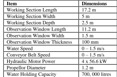
The water channel (Figure 1) is large enough to allow full-scale testing of some components, which is not possible in smaller water channels. The working section is approximately 17.2 x 5 x 2.5 m (Table 1). Water flow in the channel is controlled by suction screens, deflectors, cascade bends, wave traps, flow screens, vortex generators and a boundary layer duct in an effort to obtain flow uniformity. A conveyor belt forms the floor of the working section and moves at the same speed as the water flow to simulate friction along the sea-bed and to minimise the boundary layer .

Figure 1: Schematic of the AMHRC circulating water channel

An optimally designed flume tank will have a contraction at the inlet to the working section to ensure a steady, uniform flow [3]. However, the AMHRC water channel has a diffusing section before the inlet to the working section. This results in poor uniformity of the vertical velocity profile, particularly along the bottom of the working section. A honeycomb screen, made from short PVC pipe sections with a wire mesh screen at its downstream end is the major flow conditioning device. The honeycomb screen straightens the flow and reduces lateral turbulence and velocity, while the screen reduces turbulence in the axial direction and slows down higher velocities more than lower velocities, thereby improving flow uniformity. Errors in the manufacture of these screens mean that there are major variations in the vertical flow profile in the working section. The aim of this project was to suggest possible design changes that will lead to an improvement in the vertical uniformity of the flow in the working section of the water channel.

Item Dimensions

Working Section Length 17.2 m Working Section Width 5 m Working Section Depth 2.5 m Observation Window Length 11.2 m Observation Window Width 1.5 m Observation Window Thickness 100 mm

Water Speed 0 – 1.5 m/s

Conveyor Belt Speed 0 – 1.5 m/s

Hydraulic Motor Power 4 x 56.6 kW

Propellor Diameter 1.2 m

Water Holding Capacity 700, 000 litres Table 1: Dimensions of the circulating water channel [1].

Previous Research

A UTAS Honours Thesis was undertaken by Sean Tucker in 1995 to investigate the effects of the upper cascade bend on the flow profile in the final diffuser and inlet to working section [2]. A perspex model was constructed at 1/10th scale. Owing to the uniformity of flow in the horizontal direction, only a quarter of the flume tank width was modelled. The main body of the model was constructed from 10 mm plexiglass, the turning vanes were constructed from brass circular sections, and the honeycomb was modelled with a perforated section.

The model was tested using air rather than water. Air is less dense than water and therefore less power is required to operate the system [2]. Due to the much higher kinematic viscosity of air, it was not possible to achieve the same Reynolds number on the wind-tunnel model as in the actual flume tank. At maximum operating capacity of 0.53m3_{/s, a Reynolds number one third of} the actual flume tank was acheived. The error associated with this is not expected to be significant [2]. Results indicated that vane angle has a significant effect on flow in the working section.

Model Geometry

2-7 December 2007

Figure 2: CAD geometry of the portion of the wind tunnel used for CFD analysis.

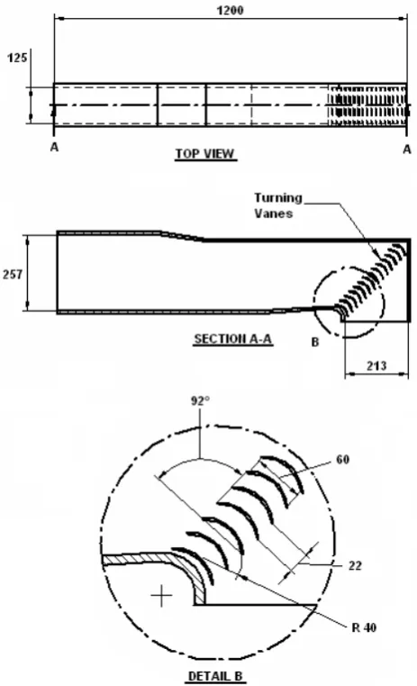
The software program ANSYS Workbench [6] was used to generate the mesh required for the CFD solution. Modelling of the vanes as 2D ‘thin walls’ prevented convergence errors associated with high-aspect ratio elements on the edge of the 2mm thick vanes. The final geometry as created in Solid Edge and modified in ANSYS Workbench is shown in Figure 3.

Figure 3: The final geometry of the wind-tunnel model

An unstructured tetrahedral mesh was used throughout the body except in near wall regions where an inflated boundary has been defined. Unstructured meshes have advantages over structured grids in that they are easier to set up and generate. An inflated boundary is required in the vicinity of the walls in order to resolve the boundary layers that are present along any zero slip surface. Figure 4 shows the inflated boundary at the outlet of the working section. The flow straightening screen was modelled by a stream-wise loss coefficient, determined from experimental results [2].

Figure 4: Inflated boundary (rectangular elements) at the outlet of the working section.

Mesh Spacing

Appropriate mesh spacing is a compromise between accuracy and available computational power. A number of mesh spacings were examined. An approximately linear relationship was found to exist between the number of nodes in the mesh and the required CPU computation time.

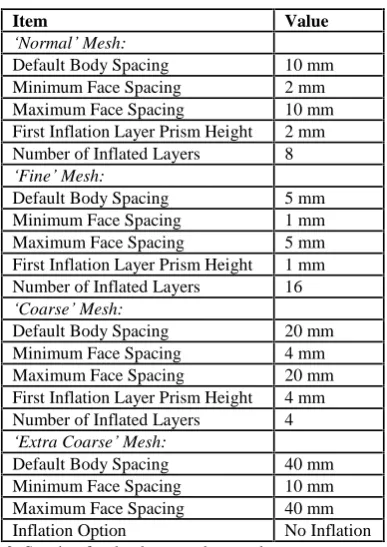
In order to ensure the chosen mesh spacing (‘normal’) results in a suitably low amount of discretisation error, three other mesh spacings were evaluated (Table 2). Each mesh was compared to the ‘normal’ mesh spacing. Velocity profiles for the chosen mesh spacings were obtained and compared with that of the ‘normal’

mesh spacing (Figure 5). All velocity profiles produced in this study were normalised as a comparison of profile ‘shape’ was required, rather than comparisons of actual velocity magnitude. For the fine mesh, computation time increased dramatically. The solution appeared to approach convergence between the coarse and normal mesh, so a result was not obtained for the fine mesh.

0 50 100 150 200 250 300

0 0.1 0.2 0.3 0.4 0.5 0.6 0.7 0.8 0.9 1 1.1

U/Umax

H

e

ig

h

t

fr

o

m

f

lo

o

r

(m

m

)

normal mesh coarse mesh extra coarse mesh

2-7 December 2007

Item Value

‘Normal’ Mesh:

Default Body Spacing 10 mm

Minimum Face Spacing 2 mm

Maximum Face Spacing 10 mm

First Inflation Layer Prism Height 2 mm Number of Inflated Layers 8 ‘Fine’ Mesh:

Default Body Spacing 5 mm

Minimum Face Spacing 1 mm

Maximum Face Spacing 5 mm

First Inflation Layer Prism Height 1 mm Number of Inflated Layers 16 ‘Coarse’ Mesh:

Default Body Spacing 20 mm

Minimum Face Spacing 4 mm

Maximum Face Spacing 20 mm

First Inflation Layer Prism Height 4 mm Number of Inflated Layers 4 ‘Extra Coarse’ Mesh:

Default Body Spacing 40 mm

Minimum Face Spacing 10 mm

Maximum Face Spacing 40 mm

Inflation Option No Inflation

Table 2: Spacing for the three meshes used to compare discretisation errors with the chosen mesh spacing.

Boundary conditions and sensitivity analysis

Boundary conditions defined on the CFD model included; planes of symmetry on each side face to ensure the 3D model resulted in a nominally 2D solution, 2D no-slip ‘thin-wall’ elements for the turning vanes, atmospheric pressure at the outlet and a velocity profile for the inlet taken from experimental results.

A sensitivity analysis was carried out to determine the effect of altering three model parameters – convergence criteria, timescale

and turbulence model. A simulation was carried out by altering the convergence criteria from the default of 1x10-4 to 5x10-4. For the same run, the timescale was changed from an ‘auto timescale’ which uses an internally calculated physical timestep size [6]. The timestep chosen for the sensitivity analysis was a physical (fixed) timestep of 2 seconds. No significant change in output was noted. The k- turbulence model is generally used by

default for industrial applications, but is not the best model for boundary layer separation and flows over curved surfaces [6]. A comparison was therefore made with the shear stress transport model (SST). No significant difference was noted in output from these two models (Figure 6), and hence the k- model was used

for the optimisation process.

0 50 100 150 200 250 300

0 0.1 0.2 0.3 0.4 0.5 0.6 0.7 0.8 0.9 1 1.1 U/Umax H e ig h t fr o m f lo o r (m m ) k-e SST

Figure 6: Comparison between turbulence models.

Model Verification

Figure 7 shows the velocity profile at the inlet to the working section compared with the experimental profile in the wind-tunnel model measured by Tucker [2]. In the lower half of the flume, the CFD demonstrates good agreement with the experimental data, but the CFD over predicts the velocity in the upper half of the channel. The region of interest in the present study is the lower half of the channel, and it is expected that with an increased resolution of data points in the upper region of the flume, a greater understanding of the flow in this region may be obtained. 0 50 100 150 200 250 300

0 0.1 0.2 0.3 0.4 0.5 0.6 0.7 0.8 0.9 1 1.1 U/Umax H e ig h t fr o m f lo o r (m m ) CFD Experimental

Figure 7: Comparison between CFD and experimental results

Design Modifications

The use of CFD in design is an iterative process, with CFD analysis determining the conformance of the design to a stated objective. Non-conformance with the objective results in design changes and further CFD analysis, while conformance gives the optimised design solution [7]. The design objective was to improve the uniformity of the flow, without resulting in a substantial increase in pressure loss. Three simple geometry modifications were adopted and their effect on the objective was examined. Velocity contours and total pressure plots were obtained to qualitatively examine the effect of design changes.

Vane Angle Alterations

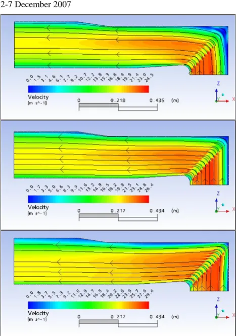
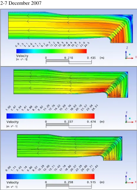
The effect of three different vane angles was examined; 92° (current design), 98° and 104°. Velocity profiles are shown in Figure 8. These profiles indicate the main area of flow improvement is along the bottom of wind-tunnel, with an angle of 104° giving the best improvement. Velocity plots and streamlines are shown in Figure 9. They suggest that an angle of 92° results in a case of ‘underturning’[8], while 104° results in ‘overturning’ [8] with an angle of 98° between the two. An angle

of 92° gives the lowest pressure drop, 104° the highest.

0 50 100 150 200 250 300

0 0.1 0.2 0.3 0.4 0.5 0.6 0.7 0.8 0.9 1 1.1

U/Umax H e ig h t fr o m f lo o r (m m ) 92° 98° 104°

2-7 December 2007

Figure 9: Velocity plots and streamlines for vane angles of 92° (top), 98° (middle) and 104° (bottom).

Honeycomb screen alterations

The effect of five different screen resistance coefficients was examined; k = 0 (no screen) and k = 2.5, 10, 20, 40. Velocity profiles are shown in Figure 10. The increase in screen resistance is similar to the effect of adding wire mesh screens to the honeycomb screen, as the flow resistance of a wire mesh screen is usually much larger than for a honeycomb. Wire mesh screens tend to increase flow uniformity due to the higher velocities being affected to a greater degree than the lower velocities. The velocity profile (Figure 10) indicates increasing flow uniformity for increased resistance coefficient. The pressure plot for k = 40 (Figure 11) indicates that pressure drop increases with improvements in flow uniformity. This is undesirable, as increased pressure drop will result in increased running costs for the circulating water channel.

0 50 100 150 200 250 300

0 0.1 0.2 0.3 0.4 0.5 0.6 0.7 0.8 0.9 1 1.1 U/Umax

H

e

ig

h

t

fr

o

m

f

lo

o

r

(m

m

)

no screen k = 2.5 k = 10 k = 20 k = 40

Figure 10: Comparison of the velocity profiles obtained for varying screen resistance coefficient.

Figure 11: Total pressure for resistance coefficient k = 40.

Vane Trailing Edge Extensions

The effect of adding trailing edge extensions to the turning vanes was examined for three different cases – no extension, an

extension of 20 mm and an extension of 40 mm. Velocity profiles are shown in Figure 13. The velocity profile obtained using this design change is more uniform than that obtained without using trailing edge extensions. Outside the boundary layer, there appears to be only about a 10% velocity gradient from the bottom of the wind-tunnel to the top. There seems to be little difference in flow profile whether extensions of 20 mm or 40 mm are used. Velocity plots and streamlines are shown in Figure 14. The pressure drop is greater with the 40 mm extensions. Owing to this, and the similarity in velocity profile between the two extension lengths, it seems the optimum design is to adopt 20 mm extensions. In comparison to vane angle and resistance screen changes, the addition of vane trailing edge extensions appears to result in the most significant improvement in flow with relatively little pressure drop.

Figure 12: Trailing edge extension design.

0 50 100 150 200 250 300

0 0.1 0.2 0.3 0.4 0.5 0.6 0.7 0.8 0.9 1 1.1

U/Umax

H

e

ig

h

t

fr

o

m

f

lo

o

r

(m

m

)

no extenions 20 mm extensions 40 mm extensions

2-7 December 2007

Figure 14: Velocity and streamlines for trailing edge extensions 0 mm, (top), 20 mm (middle) and 40 mm (bottom).

Project Limitations

The exact size, spacing and angle of turning vanes has a significant effect on the downstream flow. Minor differences between CFD and experimental turning vanes may have contributed to some of the difference between experimental and CFD velocity profiles shown in Figure 7. The phenomenon of separation is also highly important. Separation is likely to occur on the turning vanes and at the corners leading to diffusing sections. Experimental results are indicative of heavy turbulence that is not picked up properly in the CFD simulation. The time and computational power was not available to provide a sufficiently fine mesh (Figure 15) to resolve these separating flows properly. Steady improvements in computational power are resulting in the ability to solve increasingly complex problems. However, computational power continues to be a significant limitation on the accuracy of CFD.

The key objective of this research was to use CFD as a tool to optimise design modifications for the facility, not to provide a perfect prediction of flow in the facility. As a comparative design tool, that was initially shown to have reasonable agreement with experimental data in the region of interest, the analysis performed have enabled preferred modification strategies to be identified.

Figure 15: Discretisation errors in the vicinity of the turning vanes may have lead to inaccurate modelling of separation.

Future Research

Examination of further design scenarios such as smaller variations in trailing edge extension would determine the optimum value for each design alteration. Combination of the optimum of each design change and addition of new modifications such as vortex generators and roughened vanes to promote turbulence would result in an ‘overall’ optimum design.

At present, the conformance of the design to the objectives has been based on a qualitative assessment of velocity profile uniformity and pressure drop. Improvement would be gained by developing a quantitative objective statement. This would include consultation with the Australian Maritime College to determine what values of flow uniformity and pressure loss are reasonable.

The current model makes a number of assumptions that are not valid given the reality of the actual AMHRC water channel. Significant among these is the use of air rather than water. This leads to both a lower Reynolds number and the lack of a free surface that would be present on the actual circulating water channel. Future CFD models should use water as the working fluid. This would, however, come at the expense of no longer being able to use the existing wind-tunnel model for verification.

Conclusion

CFD was used as a design tool, which enabled a greater number of design changes to be investigated much more quickly than would have been possible using the existing wind-tunnel model. The wind-tunnel was useful, however, in providing a validation tool for the CFD solution in the area of interest.

Improvements in the flow uniformity could be obtained by altering the design of the circulating water channel at the Australian Maritime and Hydrodynamics Research Centre. The use of trailing edge extensions for the turning vanes, optimised turning vane angle and careful use of resistance screens could all improve the flow uniformity of the AMHRC circulating water channel and thereby increase the scope of testing that can be carried out at that facility.

References

[1] AMHRC. 2006. Circulating Water Channel (Flume Tank). Australian Maritime Hydrodynamics Research Centre. http://www.amhrc.edu.au/facilities/flumetank-info.html [2] Tucker, S. 1995. Improvement of the flow quality in the

Australian Maritime College circulating water channel. University of Tasmania Honours Thesis.

[3] Su, Y., 1991. Flow analysis and design of three-dimensional wind tunnel contractions. AIAA Journal, 29 1912 – 1920

[6] ANSYS Inc. 2005. ANSYS Workbench.

[7] Burgreen, G.W., J.F. Antaki, Z.J. Wu, and A.J. Holmes. N. D. Computational Fluid Dynamics as a Development Tool for Rotary Blood Pumps. McGowan Center for Artificial Organ Development, University of Pittsburgh.