Semi-Supervised Normalized Embeddings for Fusion and Land-Use Classification of Multiple View Data

Rochester Institute of Technology

RIT Scholar Works

Theses

12-2018

Semi-Supervised Normalized Embeddings for

Fusion and Land-Use Classification of Multiple

View Data

Poppy Immel

[email protected]

Follow this and additional works at:

https://scholarworks.rit.edu/theses

This Thesis is brought to you for free and open access by RIT Scholar Works. It has been accepted for inclusion in Theses by an authorized administrator of RIT Scholar Works. For more information, please [email protected].

Recommended Citation

Semi-Supervised Normalized

Embeddings for Fusion and Land-Use

Classification of Multiple View Data

by

Poppy Immel

A Thesis submitted in Partial Fulfillment of the Requirements

for the Degree of Master of Science in Computer Science

Golisano College of Computer and Information Sciences

Rochester Institute of Technology

Semi-Supervised Normalized

Embeddings for Fusion and Land-Use

Classification of Multiple View Data

COMMITTEE APPROVAL :

Nathan D. Cahill, D.Phil., School of Mathematics, Advisor Date

Zack Butler, Ph.D., Department of Computer Science, Advisor Date

Abstract

Acknowledgments

Table of Contents

Abstract iii

Acknowledgments iv

List of Tables vii

List of Figures viii

Chapter 1. Introduction 1

Chapter 2. Background 4

2.1 Remote Sensing and Data Fusion . . . 4

2.2 Spectral Graph Theory . . . 6

2.2.1 Spectral Clustering and Graph Partitioning . . . 6

2.3 Manifold Learning . . . 8

2.3.1 Laplacian Eigenmaps . . . 8

2.3.2 Spatial-Spectral Schroedinger Eigenmaps . . . 9

2.4 Manifold Alignment . . . 10

2.4.1 Semi-supervised Manifold Alignment . . . 11

2.4.2 Manifold Alignment with Schroedinger Eigenmaps . . . 13

2.5 Classification . . . 13

2.5.1 Linear Discriminant Analysis . . . 14

2.5.2 Support Vector Machines . . . 15

2.5.3 Random Forests . . . 15

Chapter 3. Semi-Supervised Normalized Embeddings 17 3.1 Problems with SSMA/SEMA . . . 17

3.2 Proposed Solution: SSNE . . . 18

Chapter 4. Datasets and Experiment Methodology 20

4.1 Dataset . . . 20

4.2 System . . . 22

4.2.1 Classifiers . . . 23

4.3 Experiments . . . 24

4.3.1 Experiment 1 . . . 24

4.3.2 Experiment 2 . . . 25

Chapter 5. Results and Discussion 26 5.1 Experiment 1: Classifying Berlin . . . 26

5.1.1 Scenario A: Baseline . . . 26

5.1.2 Scenario B: Independent Views with Dimensionality Reduction . . . 26

5.1.3 Scenario C: Labeled Pairwise Similarities/Dissimilarities . . . 30

5.1.4 Scenario D: Similarities via Alignment . . . 33

5.2 Experiment 2: Classifying an Unknown View . . . 36

Chapter 6. Conclusion and Future Work 48

List of Tables

4.1 The seventeen types of Local Climate Zones (LCZs), sixteen of which are present in the training data. The number of ground-truth pixels for each class represents the number on the original grid. . . 22

5.1 Experiment 1, Scenario A: Classification results for SVM, LDA, and RF when training classifiers independently on each data set with no dimensionality reduction with the Berlin data split. This illustrates both the baseline OA as well as a baseline comparison between our three classifiers. . . 26

5.2 Experiment 1, Scenario B, SVM:Classification results versus baseline (Scenario A) with the use of our SVM classifier. Each performance measure is based on the maximum possible embedding dimension q. For feature-based LE/SSSE,q = 9 for both Landsat images and q = 10 for the Sentinel image. For SSNE, q = 28 for all images. The OA and kappa values remain consistence when varyinggammap; this

shows that for this data set the inclusion of spatial features does not necessarily improve classification. . . 29

5.3 Experiment 1, Scenario B, SVM: Per-class and overall classification results versus baseline (Scenario A) with the use of our SVM classifier. Each performance measure is based on the maximum possible embedding dimension q. For feature-based LS/SSSE, q = 9 for both Landsat images and q = 10 for the Sentinel image. For SSNE,q = 28 for all images. . . 29 5.4 Experiment 1, Scenario C, SSMA/SEMA: Classification results for various

choices of µ and α for SSMA/SEMA with the SVM classifier. Each performance

measure is based on the maximum possible embedding dimension q. . . 32

5.5 Experiment 1, Scenario C, SSNE: Classification results for various choices of γs,γd, andγp for SSNE with the SVM classifier. Each performance measure is based

on the maximum possible embedding dimension q. . . 32 5.6 Experiment 1, Scenario C, SVM:Per-class and overall classification results with

the use of our SVM classifier. Each performance measure is based on the maximum possible embedding dimension q= 28. . . 33

5.7 Experiment 1, Scenario D, SVM: Classification results for γs = 100 and

var-ious choices of γp. Each performance measure is based on the maximum possible

embedding dimensionq = 28. . . 34

5.8 Experiment 1, Scenario D, SVM:Per-class and overall classification results with the use of our SVM classifier. Each performance measure is based on the maximum possible embedding dimension q= 28. . . 35 5.9 Experiment 2, Berlin: The class training and testing counts and classification

results for SEMA and SSNE compared to the baseline. The emphasized values show improvement from the baseline. . . 36

List of Figures

2.1 An example of airborne and satellite collection of remote sensing [36]. . . 4

2.2 A hyperspectral image [48]. . . 5

2.3 The spectral reflectance of vegetation and terrain. [25]. . . 5

2.4 Satellite image of an area of interest (left) and the corresponding land use/land cover map. [32] . . . 6

2.5 A toy example showing that minimum cut gives a sub-optimal partitioning [46] . . . 8

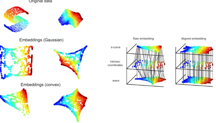
2.6 On the left, 2-dimensional embeddings of 3-dimensional surfaces (a s-curve and a wave). On the right, manifold alignment applied to two raw embeddings where the lines connecting points between each dataset represent known correspondences. The raw embeddings are projected into a latent space in which the correspondences are aligned, represented by the now straight lines from the first dataset to the section though the intrinsic coordinates [23]. . . 10

2.7 A toy example of SSMA: (a) two data sets with the same underlying distribution represented as black and red dots with labeled (blue and yellow) points; (b) the geometric structure of each dataset as a graph; (c) the similar classes are pulled together, and dissimilar classes pushed apart; (d) the aligned embedding. [50]. . . . 11

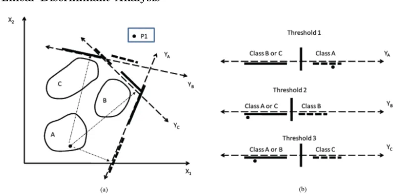
2.8 LDA can be applied to a dataset to project the data down to a lower dimensional embedding that can then be linearly separable. This example shows how a point would be classified depending on the linear discriminate [24] . . . 14

2.9 A linear support vector machine [34] . . . 15

2.10 Example of a RF classifier. (a) The training samples plotted in 2-d space. (b) Two decision trees and their corresponding learned decision boundaries for two bootstrap samples, and (c) the effect of the number of decision trees,T on the decision regions forT = 1,8,200 [15]. . . 16

4.1 Training cities: The Landsat-8 (L8-1 and L8-2) images have been rendered by selecting red, green, and blue channels to correspond to the bands having wavelengths 10.9µm, 1.6µm, and 655nm, respectively, and then by adjusting brightness, contrast, and gamma for visualization. The Sentinel-2 (S2) image has been rendered so that the red, green, and blue channels correspond to the bands having wavelengths 2.2µm, 835nm, and 665nm. . . 21

5.1 Experiment 1, Scenario A, OA: K-fold cross-validation OA of Berlin to test sensitivity of each classifier,k= 10. Note that this plot shows the results of a 90/10

training/testing data split. We see that SVM and LDA yield 2−3% higher OA

values across all views with the larger training set. However, RF yield 6−9% higher OA values across all views with the larger training set. . . 27

5.2 Experiment 1, Scenario B, LE: Classification performance (OA) on the test set for each image, after the training sets for each image have been used individually to perform feature-based LE (γp = 0) or feature-based SSSE (γp = 1, γp = 100).

The horizontal axes represent the feature dimensionq, and the baseline results from Scenario A are added to the plots for comparison. For all cases, these feature repre-sentations yield classifiers that outperform the baseline when q >6. . . 28

5.3 Experiment 1, Scenario B, SSNE, OA: Classification performance (OA) on the test set for each image, after the training sets for each image have been used to perform SSNE withS=D=∅. The horizontal axes represent the feature dimension q, and the baseline results from Scenario A are added to the plots for comparison. For all cases, these feature representations yield classifiers that outperform the baseline when the latent space has dimensionq >19. . . 28

5.4 Experiment 1, Scenario C, SSMA/SEMA:Classification performance (OA) on the test set for each image, after the training sets for each image have been used to perform SSNE with many pairwise similarities/dissimilarities. The horizontal axes represent the feature dimensionq, and the baseline results from Scenario A are added to the plots for comparison. The use of SEMA (whenα >0) appears to enable lower choices forq than SSMA (whenα= 0). . . 30

5.5 Experiment 1, Scenario C, SSNE: Classification performance (OA) on the test set for each image, after the training sets for each image have been used to perform SSNE with many pairwise similarities/dissimilarities. The horizontal axes represent the feature dimension q, and the baseline results from Scenario A are added to the plots for comparison. It is clear that the inclusion of similarities/dissimilarities (when γs, γd>0) enables much lower choices for q than Scenario B (when γs=γd= 0). . . 31

5.6 Experiment 1, Scenario C, SEMA, OA: K-fold cross-validation OA of Berlin to test sensitivity of each classifier, k= 10. Note that this plot shows the results of a 90/10 training/testing data split forα=µ= 100. . . 32

5.7 Experiment 1, Scenario C, SSNE OA: K-fold cross-validation OA of Berlin to test sensitivity of each classifier, k= 10. Note that this plot shows the results of a 90/10 training/testing data split for γs=γd=γp= 100. . . 33

5.8 Experiment 1, Scenario D: Classification performance (OA) on the test set for each image, after the training sets for each image have been used to perform SSNE with similarities provided across views for pixels in the same location andγs= 100.

The horizontal axes represent the feature dimensionq, and the baseline results from Scenario A are added to the plots for comparison. For all three images and classifiers, these feature representations yield classifiers that outperform the baseline when the latent space has dimensionq >9. . . 34

5.9 Experiment 2, Berlin: Classification map of predicted classes using the baseline method, SEMA, and SSNE for each view. . . 37

5.11 Confusion matrices of the Baseline results: We show the confusion matrices for both the Berlin and Sao Paulo classification for each view. The x-axis displays the target class; the y-axis displays the output class for all of the 16 classes present in the dataset. The lighter to darker shading represents a 0-1 classification rate of the target class for the output class. The number is the number of target class pixel classified as the output class. . . 41

5.12 Spectral Signatures of the training and testing sets for Berlin for L8-1 and L8-2: Each plot illustrates the spectral distributions for each LCZ class that is in the testing city across the training of testing cities. The training set is the combined spectral from Hong Kong, Paris, Rome, and Sao Paulo. Across the x-axis, 1 corresponds to Band 1, 2 corresponds to Band 2, etc. We can see that there is slightly less variation in the spectra signatures between the training and testing sets for L8-2 than there is for L8-1. Specifically, when looking at LCZ A. . . 42

5.13 Spectral Signatures of the training and testing sets for Sao Paulo for L8-1 and L8-2: Each plot illustrates the spectral distributions for each LCZ class that is in the testing city across the training of testing cities. The training set is the combined spectral from Berlin, Hong Kong, Paris, and Rome. Across the x-axis, 1 corresponds to Band 1, 2 corresponds to Band 2, etc. We can see that there is slightly less variation in the spectra signatures between the training and testing sets for L8-1 than there is for L8-2. . . 43

5.14 Spectral Signatures for each view: Each plot illustrates the spectral distribu-tions for each LCZ class across the five cities. Across the x-axis, 1 corresponds to Band 1, 2 corresponds to Band 2, etc. . . 44

5.15 Class Distributions for L8-1: Each histogram plot illustrates the class distribu-tions for each LCZ class. Across the columns the distribution for each city is shown. Across the rows, in the distribution for each band in the Landsat-8, view 1 images. The x-axis of each histogram shows the spectral value of each pixel, the images have been normalized to have values between 0 and 1. The y-axis represents the num-ber of counts across a small range of spectral values using MATLAB’s histogram

function. The counts are not normalized across all plots. . . 45

5.16 Class Distributions for L8-2: Each histogram plot illustrates the class distribu-tions for each LCZ class. Across the columns the distribution for each city is shown. Across the rows, in the distribution for each band in the Landsat-8, view 2 images. The x-axis of each histogram shows the spectral value of each pixel, the images have been normalized to have values between 0 and 1. The y-axis represents the num-ber of counts across a small range of spectral values using MATLAB’s histogram

function. The counts are not normalized across all plots. . . 46

Chapter 1

Introduction

In the field of remote sensing classification, the identification of specific objects or pixels in images based on spectral information, is an important task. Classification can be applied to remote sensing data in several ways including target detection, anomaly detection, and land-use classification. Target detection is used to identify where specific objects or spectra are in an image. Anomaly detection identifies where unusual patterns, such as camouflage, occur in image. Land-use classification is used to segment out areas of an image, either by region or pixelwise, and identify what type of use (i.e. forest or field) corresponds to these specific parts of the image. These tasks can be automated using machine learning so that an algorithm can learn which spectral pattern and other features correspond to a specific target or class.

However, these tasks present many challenges due to the high dimensionality of remote sensing data, the inherent properties of spectral data, and the prevalence of modal and multi-source data. First, modern sensors are capable of both multispectral and hyperspectral imaging. While a standard image captures 3 bands (red, green, and blue), multispectral sensors typically detect 3 to 15 spectral bands and hyperspectral sensors can detect hundreds of bands. This, along with the use of very high-resolution images, gives a large amount of data points (i.e. an image that ism×npixels with Lbands can be thought of as mn data points each withL features). Second, remote sensing data is difficult to interpret due to spectral variations. These phenomena can be the results of temporal variations and nonlinearities in the spectral response due to atmospheric and other environmental conditions [27]. Spectral signatures of some materials can change over time [52, 27] and some physical phenomena, such as multiple scattering, can cause a nonlinear response [4, 20, 27]. Third, the same location or city may be recorded from different angles, from different sensors and at different times giving multi-modal views. The use of different modalities can provide complementary information; however, though the data is of the same distribution, it is unaligned.

have been proposed for generating lower-dimensional data representations that are useful for clas-sification of high dimensional datasets, including Local Linear Embedding (LLE) [28], Isometric Feature Mapping (ISOMAP) [4], Kernel Principal Components Analysis (KPCA) [18], Laplacian Eigenmaps (LE) [7, 22], Diffusion Maps [14], Stochastic Proximity Embedding (SPE) [2], Local Tangent Space Analysis (LTSA) [54], t-Distributed Stochastic Neighbor Embedding (t-SNE) [51], Schroedinger Eigenmaps (SE) [8] and Spatial Spectral Schroedinger Eigenmaps (SSSE) [10].

To perform land-use classification from multi-view data, one approach would be to simply perform dimensionality reduction on each individual view and then concatenate the results. How-ever, this idea is only feasible if data from the individual views are spatially aligned and sampled in a common coordinate system. For use with multispectral and hyperspectral remote sensing data, a non-linear approach to dimensionality reduction is often appropriate due to the inherent, non-linear nature of the data. Manifold learning has been shown to successfully reduce the dimensionality of this data while preserving the nonlinearities that are captured in the data [30, 27]. Manifold alignment adapts manifold learning to compute transformations for each modality of multi-modal datasets that project the data into a common, low-dimensional embedding.

A well know algorithm for manifold learning is Laplacian Eigenmaps (LE) [7, 22]. LE is an unsupervised non-linear graph-based dimensionality reduction algorithm that uses manifold learning techniques. The goal of the algorithm is to project the original high dimensional data into a lower dimension manifold while preserving the local geometric structure of the spectral data. Schroedinger Eigenmaps (SE) [16] is a semi-supervised generalization of the Laplacian Eigenmaps algorithm which fuses both spectral and spatial information. These algorithms have been adapted to allow for manifold alignment of multi-modal data. Semi-Supervised Manifold Alignment (SSMA), like LE, preserves the local geometric structure of the spectral data from multiple sources [23, 50]. Manifold Alignment with Schroedinger Eigenmaps (SEMA) generalizes SSMA to include both spectral and spatial features [27]. Although these algorithms exhibit good general performance, they can be improved.

corresponding to the inherent spectral information of the image data. We refer to the latent space that results from the projection functions that optimize this new criterion as the Semi-Supervised Normalized Embedding (SSNE).

To validate the effectiveness of these proposed modifications, we preform land-use classi-fication to determine if the modiclassi-fications lead to improved performance. There are two inherent challenges to classification of remote sensing data. First, the underlying distribution of remote sensing data is often unknown. Second, the small number of available training samples makes it difficult to generate an accurate ground truth for remote sensing images [34, 43]. Manifold learning and manifold alignment algorithms have typically been evaluated with classification using linear discriminant analysis (LDA) [10, 17, 27, 50]. However, both support vector machines (SVM) and random forests (RF) have been utilized for classification of remote sensing imaging [6, 27, 34].

SEMA was tested using only LDA and SVMs using few images [27]. In this thesis, we propose to further evaluate SEMA along with the evaluation of our proposed algorithm, SSNE, using LDA, SVM, and RF classification algorithms. We will apply SEMA and SSNE to preprocess the multi-modal, multi-temporal, and multi-source data provided by the 2017 IEEE GRSS Data Fusion Contest [1]. We will then apply the several machine learning algorithms for land-use classification as evaluation methods. Our main results will be comparing the performance of SEMA and SSNE through various scenarios of the contest data. We compare the robustness of these algorithms through the application to different datasets in addition to the application of several classification algorithms.

Chapter 2

Background

In this chapter, we give an overview of remote sensing and spectral graph theory, a de-scription of LE, SE, SSMA, and SEMA algorithms, and an introduction to several classification algorithms. Section 2.1 gives a preliminary introduction to remote sensing and remote sensing data. In Section 2.2, we discuss spectral graph theory and spectral clustering and their relation to manifold learning. In Section 2.3, we describe the construction of LE and SE. Section 2.4, describes the how manifold learning concepts can be applied to manifold alignment via SSMA and SEMA. Finally, in Section 2.5, we describe LDA, SVM, and RF algorithms and their application to remote sensing.

2.1 Remote Sensing and Data Fusion

Remote sensing is the field of gathering information about the surface of the Earth without contact with the area of interest. Typically, remote sensing data is gathered using airborne or space sensors as show in Figure 2.1. The most common type of sensors used are optical sensors gather imagery with light from the sun.

Figure 2.1: An example of airborne and satellite collection of remote sensing [36].

Figure 2.2: A hyperspectral image [48].

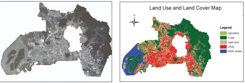
Different types of material have different spectral reflectance; for example, in Figure 2.3, we can see the spectral reflectance of three different materials. The recognition, or classification of different materials and features can be based on these spectral reflectance properties. In an-band image, the spectral reflectance curve is represented as an-dimensional feature vector at each pixel. For pixel-wise classification we can learn the representation of different materials in order to classify, for example, land cover. Figure 2.4 shows an example of a land cover map.

Figure 2.3: The spectral reflectance of vegetation and terrain. [25].

Figure 2.4: Satellite image of an area of interest (left) and the corresponding land use/land cover map. [32]

2.2 Spectral Graph Theory

An important observation to make is the relationship between spectral graph theory and the manifold learning. A graph G = {V, E} is a set of vertices V ={v1, v2, . . . , vn} and a set of

edgesE ⊆V ×V. A pair of vertices (vi, vj)∈E if there is a connection or edge betweenvi andvj.

In this application, we assume thatGis undirected, such that (vi, vj)∈E if and only if (vj, vi)∈E.

Spectral graph theory studies the properties of matrices representing graphs, including adjacency matrices and Laplacian matrices. An adjacency matrixAis defined as ann×nmatrix where each elementAi,j = 1 if (vi, vj)∈E andAi,j = 0 otherwise.

A weighted adjacency matrixW is defined elementwise byWi,j =wi,jwherewi,j represents

how strongly vi and vj are connected. If (vi, vj) 6∈E, Wi,j = 0. Note that ifG is undirected then

W must be symmetric. The degree matrix ofW,D is defined asDi,j =PjWi,j. The Laplacian

matrix L = D −W also characterizes many useful properties of a graph; these properties are described in [31]. A graph Laplacian can be normalized in several ways, most commonly as

Lsym=D−1/2LD−1/2 =I −D−1/2W D−1/2 , or (2.1)

Lrw =D−1L=I−D−1W , (2.2)

where Lsym is symmetric matrix, but Lrw is not; however, Lrw represents the Laplacian of a

graph whose weights are given by the transition probabilities of a random walk on the graph. In the next section we discuss methods of spectral clustering and graph partitioning.

2.2.1 Spectral Clustering and Graph Partitioning

Spectral clustering studies similarity graphs, a graph in which an edge vi, vj exists if some

thought of as a clustering such that a random walk stays within the same cluster instead of moving between clusters. In contrast, another justification for spectral clustering is from a perturbation theory point of view; we can consider the Laplacian matrices to be perturbations of the ideal case where the between-class similarly is zero [31].

In the domain of imagery, the vertices inGrepresent pixel values and the similarity metric is commonly defined on some distance metric between two data points in feature space. Feature space can be representative of both spectral and spatial properties. Some method used to define connectivity include mutualk-nearest neighbors,-neighborhoods, and fully connected graphs [31]. Ak-nearest neighbor graph is constructed such that each vertex is connected thekclosest vertices; in mutual k-nearest neighbors two vertices are connected if they both in each other’s nearest neighbor set. A -neighborhood graph is constructed such that pairs of vertices are connected if the distance between them is less than. In a fully connected graph all vertices are connected, and each edge is weighted according to some decreasing function of distance.

Clustering is then defined as finding the best partitions of these similarity graphs such that points in the same cluster are similar and in different clusters are dissimilar [31]. For the binary case, the goal is to partition this graph into two disjoint clusters A and B such that A∪B =V. The optimal partitioning is found by minimizing

cut(A, B) = X

vi∈A,vj∈V

wi,j. (2.3)

However, this minimization favors weakly connected outliers in the feature set. To counter this, in [45], [46] Shi and Malik propose an algorithm for instead minimizing the normalized cut

N cut(A, B) =cut(A, B)

1 vol(A) +

1 vol(B)

(2.4)

wherevol(A) =P

vi∈A,vj∈Bwi,j. Essentially, the cut is normalized so that the resulting subgraphs do not have do not have hugely different degrees allowing for a more balanced partitioning. Fig-ure 2.5 compares a minimum cut and a normalized cut on the same graph.

Equation (2.4) has been extended for multiway partition [45], [46], [53]. Supposed that we want to partition a graphV intok clustersA1∪. . .∪Ak=V; then, the k-way normalized cut can

be defined by:

kN cut(A1, . . . , Ak) =

1 k k X i=1

cut(Ai, A\Ai)

vol(Ai)

. (2.5)

Note thatkN cut(A1, A2) =N cut(A1, A2).

Further, Equation (2.5) can be rewritten in terms of the matrix Laplacian. The matrix Laplacian is defined asL=D−W whereW is the edge weight matrix andDis a diagonal degree matrix given by Di,i =PjWi,j. By forming Equation 2.5 as

kN cut(A1, . . . , Ak) =

1 k k X i=1

ciTLci

ciTDci

Figure 2.5: A toy example showing that minimum cut gives a sub-optimal partitioning [46]

where ci = v ∈ Ai. It can be see that the stationary points for each of the k clusters can be

computed from the generalized eigenproblem: LC =λDC, where ci,j = 1 ifci ∈Aj and ci,j = 0

otherwise.

It has been shown that in spectral clustering, utilizing a normalization factor such as de-scribed above or Equation 2.1 and 2.2 improves clustering [31], as opposed to using the unnormal-ized Laplacian. This directly motivates our proposed algorithm described in Chapter 3.

2.3 Manifold Learning

Manifold learning is class of non-linear methods for dimensionality reduction that seeks to preserve properties of the non-linear spectral responses that are captured in high dimensional data that implicitly lies on a manifold.

Let X = {x1, . . . ,xk} be points in Rn that represent, for example, the spectral features

of pixels in a remote sensing image. The goal of manifold learning is to create a mapping Y =

{y1, . . . ,yk}in Rm of the points in X where m << n while preserving the geometric structure of

X.

2.3.1 Laplacian Eigenmaps

Laplacian Eigenmaps (LE) is an unsupervised manifold learning technique proposed by Belkin and Niyogi in [7]. The LE algorithm preserves local neighborhoods by penalizing when neighboring points inX are mapped such that their respective points inY are far apart.

The LE algorithm consists of the following three steps:

2. Define the graph Laplacian as

L=D−W, (2.7)

whereW is an edge weight matrix andDis a diagonal degree matrix given byDi,i =PjWi,j.

Typically, W is defined by the heat kernel such that Wi,j = exp −||xi−xj||2/σ

if there exists an edge betweenxi and xj inGand Wi,j= 0 otherwise.

3. The mapping Y is given by the minimization of the objective function

Φ(F) = tr

FTXDXTF−1 FTXLXTF

, (2.8)

where tr is the trace of a matrix. One solution to Equation (2.8) can be found by solving the generalized eigenproblem

Lf =λDf (2.9)

for the smallestmsmallest non-trivial eigenvector. The pointsyT₁, . . . ,y_mT are defined by the rows of F = [f1, . . . ,fm] where f0,f1, . . .fm are ordered so that 0 =λ0 < λ1 < λ2 < . . . <

λm. We note that Equation (2.8) is similar to Equation (2.4). From this we can observe that

Ncuts and the LE algorithm have a similar form.

2.3.2 Spatial-Spectral Schroedinger Eigenmaps

Schroedinger Eigenmaps (SE), proposed by Czaja and Ehler in [16] is a semi-supervised generalization of LE that takes into consideration not just the spectral features of the image data but also the knowledge of particular classes. Spatial-Spectral Schroedinger Eigenmaps (SSSE), proposed by Cahill et al. in [10], gives an instance of SE in which the spatial proximity between pixels, i.e the spatial features, are used rather than knowledge of the class labels. SSSE follows the same procedure as LE but incorporates a potential matrix V. The potential matrix can be constructed to cause specific points to be mapped close to the origin or close to each other. These two types of potential matrices are called barriers and clusters, respectively.

A barrier potential is defined with a non-negative diagonal matrixV. Each non-negativeVi,i

pulls the corresponding ith point toward the origin. A cluster potential is the sum of non-diagonal matricesV(i,j)defined asV_i,i(i,j)=V_j,j(i,j)= 1,V_i,j(i,j)=V_j,i(i,j) =−1, andV_k,l(i,j) = 0 otherwise. In this construction, the corresponding ith and jth points are pulled closer together in the embedding. Both constructions are further described in [8], [10], and [16].

SSSE follows the same procedure as LE with a modification to Equation (2.8). The inclusion of V gives the following objective function

ΦSSSE(F) = tr

FTXDXTF−1 FTX(L+αV)XTF

(2.10)

where α is a chosen weight parameter defining the contribution of V. Like LE, a solution to Equation (2.10) can be found by solving the generalized eigenproblem

This is similar to Equation 2.9 with the addition of the weightedV potential matrix on the left side. As before in LE, we solve for them smallest non-trivial eigenvectors of Equation (2.11) which give them vectors used to construct the projection matrix to the latent space. Specifically, the points

yT₁, . . . ,y_mT ∈ Y are defined by the rows of F = [f1, . . . ,fm] where f0,f1, . . .fm are ordered so

that 0 =λ0 < λ1 < λ2 < . . . < λm.

2.4 Manifold Alignment

Laplacian Eigenmaps and Spatial-Spectral Schroedinger Eigenmaps are both dimensionality reduction algorithms that can be applied to data from a single modality. However, Ham et al. [23] uses similar techniques for manifold alignment. Manifold alignment allows for multiple datasets to be fused together. Semi supervised alignment of manifolds [23] requires partially labeled data which map to intrinsic coordinates for multiple datasets. Using these intrinsic coordinates, we can create a Laplacian matrix that encodes the labeled and unlabeled data points for each dataset. Like in LE, this method minimizes a cost function to create an optimal projection function which projects each dataset into an aligned latent space. Figure 2.6 illustrates a comparison between the raw unaligned embedding and the aligned embedding of two datasets with known correspondences. Manifold alignment seeks to project the source data into a common latent space.

2.4.1 Semi-supervised Manifold Alignment

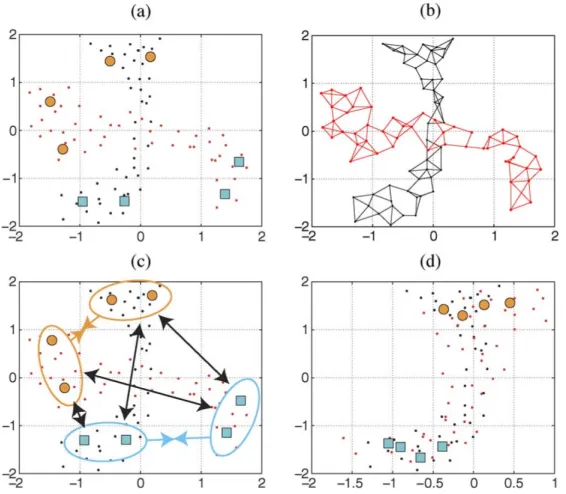
Tuia et al. [50] applied Ham’s [23] manifold alignment method to sets of hyperspectral images captured with varying angles of acquisition with an algorithm called Semi-Supervised Manifold Alignment (SSMA). These sets of images have the same underlying objects but are distorted from one another. Figure 2.7 shows a toy example of the SSMA algorithm in which two distorted datasets drawn from the same underlying distribution are aligned.

Figure 2.7: A toy example of SSMA: (a) two data sets with the same underlying distribution represented as black and red dots with labeled (blue and yellow) points; (b) the geometric structure of each dataset as a graph; (c) the similar classes are pulled together, and dissimilar classes pushed apart; (d) the aligned embedding. [50].

Consider M datasets where each datasetXm ∈ _Rdm _{contains the spectral features of the} pixel in themth image. EachXm is constructed of a set oflm labeled pairs of samples and classes

{xm_i ,ym_i } and um unlabeled samples {xmj } wherelm << um. AllM datasets can be represented

using a block diagonal matrix X where each Xm _{are placed as blocks along the diagonal of the}

matrix and all other elements are zero. For X we construct three graphs, each having a different set of weights. We refer to the Laplacian matrices of these graphs as the geometric preserving term

Lg, the similarity term Ls, and the dissimilarity term Ld.

1. For each datasetXm, the spectral geometric preserving term is constructed as

where eachW_gmis a weight matrix constructed using some distance metric on all the points in

XmandD_gmis a diagonal degree matrix withDm_g (i, i) =P

jWgm(i, j). This graph Laplacian

matrix for each domain is then used to construct a block diagonal matrix Lg.

2. Next, for each dataset the similarity Laplacian matrix is constructed as

Lm_s =Dm_s −W_sm (2.13)

where W_sm(i, j) = 1 if xm_i and xm_j have the same label and W_sm(i, j) = 0 otherwise, and Dm

s (i, i) =

P

jWsm(i, j). This graph Laplacian matrix for each dataset is used to construct a

block diagonal matrix Ls.

3. Finally, for each data set the dissimilarity Laplacian matrix is constructed as

Lm_d =Dm_d −W_dm (2.14)

where W_dm(i, j) = 1 if xm_i and xm_j have different labels and W_dm(i, j) = 0 otherwise, and D_dm(ii) =P

jWdm(ij). This graph Laplacian matrix for each dataset is used to construct a

block diagonal matrix Ld.

Now, the goal of SSMA is to create a projection matrixfm∈_Rdm×dm _{for each dataset that} will project the points in Xm to a latent spaceF. This is done by simultaneously minimizing the distances between similar classes and maximizing the distance between dissimilar classes with the objective function:

ΦSSMA(F) = tr

FTXLdXTF

−1

FTX(Ls+µLg)XTF

(2.15)

where F is our dmax×dmax projection matrix with dmax =Pmdm and µ is a chosen parameter

that determines how much the geometric term is considered.

The minimization can be solved using a generalized eigenvalue problem:

X(Ls+µLg)XTf =λX(Ld)XTf (2.16)

by computing thedmaxsmallest non-trivial eigenvalues. Specifically, the pointsyT₁, . . . ,y_mT

are defined by the rows ofF = [f1, . . . ,fdmax] wheref0,f1, . . .fdmax are ordered so that 0 =λ0<

λ1< λ2 < . . . < λdmax. The projection for each source domain to the latent space is given by

P_F(Xm) =f_mTXm. (2.17)

2.4.2 Manifold Alignment with Schroedinger Eigenmaps

SSMA creates a projection function based solely on the spectral properties of the imagery. Manifold Alignment with Schroedinger Eigenmaps (SEMA) is an algorithm proposed by Johnson, et al. [27] that builds on SSMA by considering the spatial properties of the images in the optimal cost function. As with the SSSE generalization of LE, this is done by constructing a potential termV that preserves the spatial neighbors of each image.

SEMA generalizes the cost function in Equation (2.15) with the inclusion of the potential termV in the numerator. The new cost function is given as

ΦSEMA(F) = tr

FTXLdXTF

−1

FTX(Ls+µ(Lg+αV))XTF

(2.18)

The projection can be computed using the same procedure as SSMA: by solving the modified generalized eigenvalue problem

X(LS+µ(Lg+αV))XTγ =λX(Ld)XTγ (2.19)

for thedmax smallest eigenvalues. As before, the corresponding eigenvectors are used to construct

a projection matrix for each dataset. Specifically, the pointsy₁T, . . . ,yT_m are defined by the rows of

F = [f1, . . . ,fdmax] where f0,f1, . . .fdmax are ordered so that 0 = λ0 < λ1 < λ2 < . . . < λdmax. The projection for each source domain to the latent space is given by

P_F(Xm) =f_mTXm. (2.20)

This method allows for the fusion of spatial and spectral information of the datasets to be used for manifold alignment.

2.5 Classification

The algorithms described in Sections 2.3 and 2.4 consider the problem of dimensionality reduction and data fusion. We now consider when the data is representative of multiple categories or classes. Classification is the problem of using characteristic of the data to predict the classification of each sample in a dataset. A classifier can be trained on a set of known sample and class pairs such that it can be applied predictively to determine the class of unknown samples in the same feature space. Preprocessing techniques, such as dimensionality reduction and data fusion, can be performed on a dataset prior to classification in order to reduce computation time and allow for consistent data.

for classification: typically, there are only a small number of training samples available, and the distribution of each band is often unknown. We discuss an overview of Linear Discriminant Analysis (LDA), support vector machines (SVM), and random forests (RF) and previous applications of these classifiers to remote sensing data.

2.5.1 Linear Discriminant Analysis

Figure 2.8: LDA can be applied to a dataset to project the data down to a lower dimensional embedding that can then be linearly separable. This example shows how a point would be classified depending on the linear discriminate [24]

Linear Discriminant Analysis (LDA), a generalization of Fisher’s linear discriminant, is a method of linear transformation that maximizes class separation based on the conditional proba-bility densities of the class distributions. This algorithm is commonly used for both dimensionality reduction and classification. For this we discuss LDA as a classification algorithm. LDA computes the linear discriminants that represent the best directions that maximizes the separation of classes. These linear discriminants are computed from the eigenvalues and eigenvectors of the scatter ma-trices, which characterize the between-class and within-class scatter. These scatter matrices are defined by the covariance of the class means.

Figure 2.9: A linear support vector machine [34]

2.5.2 Support Vector Machines

A support vector machine (SVM) is a supervised machine learning technique. The goal of an SVM is to find a hyperplane or decision boundary that separates data into discrete classes; see Figure 2.9. The optimal decision boundary is learned by iteratively minimizing misclassification of labeled training samples. An SVM is classically a binary classifier, but in practice an SVM can be used for multi-class problems by combining multiple binary SVMs. Further, a linear SVM assumes that the classes are linearly separable, but in cases where class clusters overlap one another or are not linearly separable, a kernel function can be incorporated. This will project nonlinear data into a higher dimension in which the classes can be separated linearly.

Support vector machines are ideal for classification problems in the remote sensing field for two reasons: SVMs makes no assumptions about the underlying probability distribution and have been shown to have high accuracy on small training sets [34], [43]. SVMs have been used for classification in several remote sensing applications including [27], [33] and [56].

2.5.3 Random Forests

Unlike binary SVM, which create a single hyperplane decision boundary that separates the data into two classes, decision trees create decision boundaries based on hierarchical rules. This essentially partitions the feature space with multiple decision boundaries.

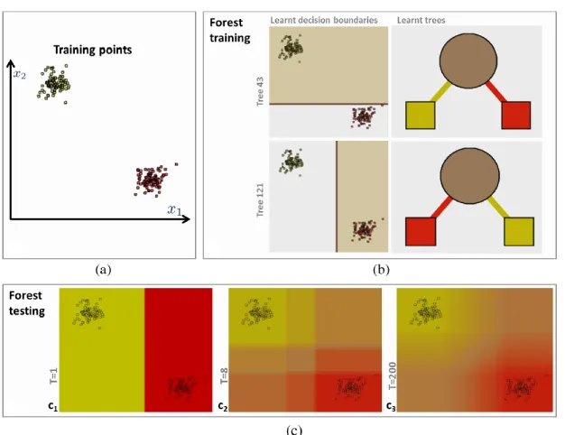
Figure 2.10: Example of a RF classifier. (a) The training samples plotted in 2-d space. (b) Two decision trees and their corresponding learned decision boundaries for two bootstrap samples, and (c) the effect of the number of decision trees, T on the decision regions forT = 1,8,200 [15].

such that at each node, the best split is computed, where a split is a partitioning on a single attribute. The value of the split is computed as the sum of the squared error of the resulting attribute split. This procedure is usually done using a greedy algorithm, adding nodes until splitting no longer improves prediction. Decision trees are subject to overfitting, but there are several ways to overcome this including pruning, where nodes are iteratively removed from the tree if they do not affect prediction, and ensemble methods, where multiple decision trees are created. Random Forests (RF) are one such ensemble method.

RF classifiers create several decision trees each based on a bootstrap sample of the training data. A bootstrap sample is a random sampling with replacement of the dataset. An RF classifier preforms the following procedurek times. 1) Draw a bootstrap sample from the data. 2) Train a decision tree using this sample set. A prediction is then made with a majority vote among the k trees. Figure 2.10 shows an example of a RF classifier.

Chapter 3

Semi-Supervised Normalized Embeddings

Both SSMA and SEMA are manifold alignment algorithms that have been shown to suc-cessfully fuse multi-modal remote sensing image data and reduce dimension as a preprocessing step for classification. However, we propose an improved algorithm. In Section 3.1, we discuss some problems with SSMA/SEMA. In Section 3.2, we propose our algorithm as a solution to these problems. In Section 3.3 we discuss the computational complexity of our algorithm.

3.1 Problems with SSMA/SEMA

The cost functions, Equations (2.16) and (2.19), described in Section 2.4 are minimized to compute projections function for projecting each dataset into the latent, aligned space. These cost functions are based on the use of Laplacian graph matrices to encode the spectral, spatial, and expert-labeled class information. An objective function Φ(F) for both SSMA and SEMA are defined as:

ΦSSMA(F) = tr

FTXLdXTF

−1

FTX(Ls+µLg)XTF

, or (3.1)

ΦSEMA(F) = tr

FTXLdXTF

−1

FTX(Ls+µ(Lg+αLp))XTF

, (3.2)

whereXis the raw unaligned data,Fis the matrix used to project this data into the aligned latent space, Lg is the Laplacian encoding of the spectral information, Lp is the Laplacian encoding of

the spatial information,Ld is the Laplacian encoding of the provided dissimilarity pairs, Ls is the

Laplacian encoding of the provided similarity pairs, andµandαare chosen parameters that weight the influence ofLg and Lp.

Both ΦSSMA and ΦSEMA can be expressed in the form:

Φ(F) = tr

FTXLBXTF

−1

FTXLAXTF

, (3.3)

where LA and LB are graph Laplacians, and so under the assumption that XLBXT is

invert-ible, Φ(F) has a family of minima characterized by a set of µ₁, . . ., µ_d and λ1, . . ., λd be the

generalized eigenvectors and corresponding generalized eigenvalues of XLAXT,XLBXT

(i.e., they satisfy XLAXTµi = λiXLBXTµi), sorted such that λ1 ≤ . . . ≤λd and normalized so that

µT_i XLBXTµi = 1, i= 1, . . . , d. Then, (3.3) has a local minimum value of

Pq

i=1λi for any Fˆ of

the form Fˆ =MQT, where M=

µ₁, . . . ,µ_q

Upon examination, they are clearly unsuitable if no similarity or dissimilarity pairs are provided. In this case, Ld = 0, where Ld is the encoding of dissimilarity pairs as a Laplacian

matrix, and so FTXLdXTF=0, in which case Φ(F) diverges and cannot be minimized. Even if

some dissimilarity pairs are provided, this may still be problematic. We note that by construction, rank(Ld)≤ |D|, whereDis the degree matrix corresponding to the weighted adjacency matrixW,

then rank FTXLdXTF

≤ |D|. Therefore, if fewer thanq, whereq is the number of dimensions in the embedding, dissimilarity pairs are provided, FT_XL

dXTF is guaranteed to be singular.

Ideally, we would like to pose an objective function that exhibits similar behavior to ΦSSMA

or ΦSEMA whenFTXLdXTFis invertible, but that also gives meaningful projections into a latent

space whenFTXLdXTFis singular. Furthermore, if no expert information is provided at all (i.e.,

when|S|=|D|= 0), such an objective function should revert to one that behaves like an objective function from some “standard” dimensionality technique that is applied independently to each view,

To focus on this last point first, we argue that if no expert information is provided at all, then appropriate objective functions to minimize would be either:

ΦLE(F) = tr

FTXDgXTF

−1

FTXLgXTF

, or (3.4)

ΦSSSE(F) = tr

FTXDgXTF

−1

FTX(Lg+αLp)XTF

, (3.5)

which are essentially feature-based multi-view versions of the objective functions minimized in the Laplacian Eigenmaps [7] and Spatial-Spectral Schroedinger Eigenmaps [10] methods. Note that XDgXT is positive definite and hence invertible (assumingX is full rank), and so the minima of

Equations (3.4)–(3.5) can be found by using the solution of the generalized eigenvector problems.

3.2 Proposed Solution: SSNE

Next, we introduce a normalization term to these objective functions. As described in Section 2.2, in the domain of spectral clustering it has been shown that the use of normalized Laplacians improves clustering results. The most common way to normalize Laplacian is to nor-malize the Laplacian matrix by is corresponding degree matrix. Hence, in order to incorporate a normalization term into Equations (3.1)–(3.2) we add there Dg into objective functions. Both

types of new objective function take the form:

ΦSSNE(F) = tr

FTX(Dg+γdLd)XTF

−1

FTX(Lg+γsLs+γpLp)XTF

, (3.6)

whereγd,γs, andγp are chosen parameters that weight the influence ofLs,LdandLp. We can see

that ΦSSNE reduces to ΦLE when γd=γs =γp = 0 and to ΦSSSE when γd=γs = 0 and γp =α.

SinceDg+γdLdis guaranteed to be positive definite forγd≥0, the minimum of (3.6) can be found

by solving a generalized eigenvector problem defined as

by computing the dmax smallest non-trivial eigenvalues. The projection for each source domain

corresponds to the row blocks of Fsuch thatF= [f1,f2, ...,fdmax].

Using this optimal solution to project into the latent space yields the Semi-Supervised Normalized Embedding (SSNE).

3.3 Computational Complexity

As with SSMA and SEMA, the algorithm for computing SSNE depends mainly on the construction of weighted adjacency matrixes, the construction of graph Laplacian matrices and then computing the generalized eigenvalue decomposition. As described in [27], the complexity of SEMA is given by four parts. First, the computation of the spectral similarities and dissimilarities: O(DNlog(k) log(N)); second, the computation of the spatial similarities: O(Nlog(ksp) log(N));

third, the solution of the generalized eigenvalue: O(DN k3_{); and fourth, obtaining the d smallest}

non trivial eigenvalues: O(DN2), where Dis the original dimension of the data, N is the number of data points, k is the number the number of spectral nearest neighbors, ksp is the number of

spatial nearest neighbors, and d is the desired embedded dimensionality. The full derivation of these computation complexity is described in [27]. Since SSNE only includes the addition of a single term,Dg that must already be computed to constructLg, the complexity will be that same

Chapter 4

Datasets and Experiment Methodology

In [26, 27] it has been shown that, as a preprocessing step, SSMA and SEMA improve accuracy for classification of remote sensing imagery. Throughout the experiments posed in the thesis, we further demonstrate the effectiveness of SEMA and evaluate our proposed algorithm SSNE. We test on the multi-modal, multispectral data set provided by the 2017 IEEE GRSS Data Fusion Contest. Using the data provided we evaluate both SEMA and SSNE through exploring the parameter space of these algorithms. Further we evaluate the robustness of SSNE by using several subsets of the contest data and application of several classification algorithms.

In this chapter, we first describe the contest data in full in Section 4.1, then we describe the basic system that we will follow for all experiments in Section 4.2, and finally we describe the specific experiments we will perform in Section 4.3.

4.1 Dataset

The 2017 IEEE GRSS Data Fusion Contest [1] provides a multi-modal, multi-temporal, multi-source dataset for exploring land-use classification algorithms. The dataset is split into a set of five training cities: Berlin, Hong Kong, Paris, Rome, and Sao Paulo, and a set of four testing cities: Amsterdam, Chicago, Madrid, and Xian. Several datasets are provided for each city which include: 2-4 Landsat-8 with 9 bands provided, resampled to 100m resolution; a Sentinel-2 with 10 bands provided, resampled to 100m resolution; and three Open Street Map (OSM) layers with land use and building information provided as raster layers at 20m resolution. For the training cities there are ground truth maps for land-use, using classes defined in terms of Local Climate Zones (LCZ) [47, 5], which include ten urban classes and seven rural classes. These ground truth maps are provided as rasters with 100m resolution. For each city, all data has been spatially registered.

Berlin

Hong

Kong

P

aris

Rome

Sao

P

aulo

Landsat-8-1 Landsat-8-2 Sentinel-2 ground truth

Table 4.1: The seventeen types of Local Climate Zones (LCZs), sixteen of which are present in the training data. The number of ground-truth pixels for each class represents the number on the original grid.

# GT Pixels

LCZ Type Berlin Hong Kong Paris Rome Sao Paulo

1 Compact High-rise −− 631 56 −− 955

2 Compact Midrise 1534 179 2705 1551 134

3 Compact Low-rise −− 326 −− 104 5308

4 Open High-rise 577 673 366 −− 482

5 Open Midrise 2448 126 446 1495 244

6 Open Low-rise 4010 120 2419 480 1862

7 Lightweight Low-rise −− −− −− −− −−

8 Large Low-rise 1654 137 748 435 1915

9 Sparsely Built 761 −− 60 −− 335

10 Heavy Industry −− 219 −− 51 179

A Dense Trees 4960 1616 4497 284 6359

B Scattered Trees 1028 407 394 555 302

C Bush, Scrub 1050 691 −− −− −−

D Low Plants 4424 568 7688 984 376

E Bare Rock or Paved −− −− 214 −− 109

F Bare Soil or Sand 359 −− −− −− 144

G Water 1732 2379 234 500 3492

4.2 System

The provided ground truth for each image in the 2017 IEEE GRSS Data Fusion Contest data will be divided into a training and testing set. Using the labeled points given by the training set, the images will be aligned using a manifold alignment algorithm. The datasets will be projected into a latent space using a manifold alignment technique in which a classifier will be trained. The points in the testing set, projected into the latent space, will be classified using this classier and compared to the ground truth values. The manifold alignment algorithms used are LE/SSSE, SSMA/SEMA, and SSNE. For classification we use a linear discriminant analysis classifier (LDA), a support vector machine (SVM), and a random forest (RF) classifier. Figure 4.2 shows a flowchart of this process.

Specifically, the pixels in L8-1, L8-2, and S2 corresponding to the training set form the three-view data for each city in X(1), X(2), and X(3), respectively, and the pixels in each image corresponding to the test set are stored inXe(1),Xe(2), andXe(3). Since all images are registered, X(1),

X(2)_{, and X}(3) _{share a common set of class labels Y, and}

e

X(1)_,

e

X(2)_{, and}

e

X(3) _{share a common set}

Figure 4.2: Flowchart of General Experiment Pipeline: (a) The original n datasets also referred to as views. (b) The split of labeled ground truth points into independent training and testing sets. (c) Manifold alignment is applied to the raw data and the training and testing data is projected into an aligned latent space. (d) A classifier is then trained on the now aligned training data. The trained classifier is used to predict the classes of the testing data.

4.2.1 Classifiers

In addition to comparing manifold alignment algorithms we show their robustness to differ-ent classification algorithms. We compare three classifiers: a linear discriminant analysis classifier (LDA), a support vector machine (SVM), and a random forest (RF) classifier.

The LDA classifier was implemented and used for analysis of manifold alignment [10, 26, 27].

The SVM is one-versus all; it uses Gaussian RBF kernels as implemented in MATLAB’s fitcsvm

function, and it employs the heuristic procedure available in fitcsvm in order to automatically determine the kernel scaling. The implementation of the SVM classifier used is identical to that

used in [26, 27]. The random forest was implemented using scikit-learns’s

4.3 Experiments

We propose two sets of experiments: the first shows the performance of SEMA and SSNE for four scenarios and compares classifiers, and the second applies manifold learning to the task of classifying unknown views.

4.3.1 Experiment 1

For this experiment, we utilize the data from a single city, Berlin. We use versions of the two Berlin Landsat-8 images (denotedL8-1 andL8-2) and the Sentinel-2 image (denotedS2) that are down sampled versions of the originals in which every other row and column are removed. (This is done for computational expediency.) Furthermore, we normalize the pixel values so that the spectra at each pixel has unit norm. The down sampled version of the ground truth is split into training/testing sets by randomly sampling 50% of the ground truth pixels in each class for training and reserving the remaining pixels for testing. This yields a training/testing split of 3061/3060 pixels across 12 classes. The pixels in L8-1, L8-2, and S2 corresponding to the training set form the three-view data in X(1), X(2), and X(3), respectively, and the pixels in each image corresponding to the test set are stored inXe(1),Xe(2), andXe(3). Since all images are registered, X(1),

X(2)_{, andX}(3) _{share a common set of class labels Y={y}

j|j = 1, . . . ,3061}, andXe(1),Xe(2), andXe(3) share a common set of class labelsYe={y˜_j|j = 1, . . . ,3060}.

We describe a number of possible scenarios we will investigate for exploiting multiple view data for land use classification. Across all scenarios, we use the same training/testing split, and we use only the training data to compute projections into a latent space using SSNE, SSMA, or SEMA. Once the training data is projected, it is used to train one-versus-all support vector machine (SVM) classifiers. The testing data is then projected into the latent space, and class labels are predicted using our three classifiers: LDA, SVM, RF.

The scenarios we explore are as follows:

• Scenario A: Baseline: All views are treated independently, and no dimensionality reduction / data fusion is performed. Separate classifiers are trained directly on the data inX(1),X(2), and X(3), respectively.

• Scenario B: Independent Views with Dimensionality Reduction: All views are

treated independently, so thatS=D=∅. Dimensionality reduction is performed via SSNE withγs=γd= 0. If γp = 0, this is roughly equivalent to performing a feature-based version

of Laplacian Eigenmaps independently on each view; if γp >0, this is roughly equivalent to

performing independent feature-based versions of SSSE on each view. (The “rough” equiva-lence is because SSNE would project the data from each image into a 9- or 10-dimensional subspace of R28, whereas feature-based LE or SSSE would project the data directly into R9

• Scenario C: Labeled Pairwise Similarities/Dissimilarities: For each of the 12 classes, one pair of pixels (in different spatial locations) is randomly selected and assigned as a sim-ilarity in S1,2, one pair in S1,3, and one pair in S2,3. This simulates a scenario in which an

expert analyst would manually identify, for each class, a point inX(i)and a different point in

X(j) _{that both belong to the same class. The analyst would therefore be required to manually}

identify 36 pairs of points. The dissimilarity set is automatically constructed by populating it with pairs of identified points that are from different classes. SSNE, SSMA, and SEMA are all possible in this scenario.

• Scenario D: Similarities via Alignment: Registration and resampling of the images into a common coordinate system is exploited by defining similarities between pixels from each view that share the same spatial location. Specifically, Si,j =

n

x(si),x(sj)

s= 1, . . . ,3061 o

, 1≤i, j ≤3, i6=j. No dissimilarities are provided, so neither SSMA nor SEMA are possible in this scenario. Note that this is the only scenario in which the spatial alignment of the multiple view data is exploited.

4.3.2 Experiment 2

Next, we expand our dataset to include all five training cities from the contest data. We use versions of the two Landsat-8 images (denoted L8-1 and L8-2) and the Sentinel-2 image (denoted S2) for each city (totaling 15 views). Each view is a down sampled version of the originals in which every other row and column are removed, and the pixel values have been normalized so that the spectra at each pixel has unit norm.

We perform two scenarios. First, we use the data from four cities: Hong Kong, Paris, Rome, and Sao Paulo, to align the three views (L8-1, L8-2, S2) and train an SVM classifier. With this classifier, we predict the classes of the pixels in the Berlin image that correspond to points with a class label provided by the contest. Second, we use the data from four cities: Berlin, Hong Kong, Paris, and Rome to align the views and train an SVM classifier in order to predict the classes of the pixels in the Sao Paulo image that correspond to points with a class label provided by the contest. We run this experiment of two cities since the class distributions, and consequently the training/testing split, vary between each city.

Chapter 5

Results and Discussion

For each scenario in each experiment, we report two classification performance measures for the test data: overall accuracy (OA) and kappa coefficient (κ). Overall accuracy is defined as ratio of the total number of correctly-predicted class labels to the total number of test points evaluated. Kappa coefficient is defined in Senseman et al. [44] and measures the improvement of a classification result over the result that would be achieved by random assignment of class labels.

5.1 Experiment 1: Classifying Berlin

5.1.1 Scenario A: Baseline

When training classifiers independently on each data set with no dimensionality reduction, the resulting OA values for the test data are shown in Table 5.1. It is clear from these baseline values that the raw data available from the Landsat images are better able to predict land use than the raw data from the Sentinel image.

Table 5.1: Experiment 1, Scenario A: Classification results for SVM, LDA, and RF when

training classifiers independently on each data set with no dimensionality reduction with the Berlin data split. This illustrates both the baseline OA as well as a baseline comparison between our three classifiers.

Classifier OA κ

L8-1 L8-2 S2 L8-1 L8-2 S2

SVM 0.8268 0.8072 0.7428 0.8000 0.7769 0.7009

LDA 0.7327 0.7314 0.6997 0.6925 0.6895 0.6508

RF 0.7324 0.7418 0.6840 0.6867 0.6985 0.6271

In addition, we can see that using an SVM yields higher OA and κ values for all three views. Figure 5.1 shows the results of k-fold cross-validation for each classifier. Again, we see that the Landsat-8 images have slightly higher OA values than the Sentinel-2 image. Comparing classification methods, SVM consistently preforms the best.

5.1.2 Scenario B: Independent Views with Dimensionality Reduction

L8-1 L8-2 S2

Figure 5.1: Experiment 1, Scenario A, OA:K-fold cross-validation OA of Berlin to test sensi-tivity of each classifier, k= 10. Note that this plot shows the results of a 90/10 training/testing data split. We see that SVM and LDA yield 2−3% higher OA values across all views with the larger training set. However, RF yield 6−9% higher OA values across all views with the larger training set.

view, yielding three separate generalized eigenvector problems. The second is to perform SSNE under the assumption that there are no similarities or dissimilarities, yielding one block diagonal generalized eigenvector problem. From a theoretical point of view, the only difference between these two approaches is that the first will yield three separate “latent” spaces, whereas the second will yield one larger-dimensional latent space which contains three orthogonal subspaces representing the embeddings of each view.

Figures 5.2–5.3 illustrate classification results from both approaches. Further, these figures compare the sensitivity over different γp values, which weights the contribution of spatial feature,

L8-1 L8-2 S2

SVM

LD

A

RF

q q q

Figure 5.2: Experiment 1, Scenario B, LE:Classification performance (OA) on the test set for each image, after the training sets for each image have been used individually to perform feature-based LE (γp = 0) or feature-based SSSE (γp = 1, γp = 100). The horizontal axes represent the

feature dimensionq, and the baseline results from Scenario A are added to the plots for comparison. For all cases, these feature representations yield classifiers that outperform the baseline whenq >6.

L8-1 L8-2 S2

SVM

LD

A

RF

q q q

Figure 5.3: Experiment 1, Scenario B, SSNE, OA: Classification performance (OA) on the

test set for each image, after the training sets for each image have been used to perform SSNE with

Table 5.2: Experiment 1, Scenario B, SVM:Classification results versus baseline (Scenario A) with the use of our SVM classifier. Each performance measure is based on the maximum possible embedding dimensionq. For feature-based LE/SSSE,q = 9 for both Landsat images andq= 10 for the Sentinel image. For SSNE,q = 28 for all images. The OA andkappavalues remain consistence when varying gammap; this shows that for this data set the inclusion of spatial features does not

necessarily improve classification.

Feature-based LE/SSSE SSNE with S=D=∅ Baseline (Scenario A)

Measure γp L8-1 L8-2 S2 L8-1 L8-2 S2 L8-1 L8-2 S2

OA

0 0.8621 0.8382 0.7582 0.8611 0.8386 0.7627

1 0.8650 0.8451 0.7611 0.8647 0.8425 0.7660 0.8268 0.8072 0.7428

100 0.8670 0.8474 0.7572 0.8663 0.8425 0.7634

κ

0 0.8409 0.8133 0.7190 0.8398 0.8136 0.7239

1 0.8443 0.8213 0.7225 0.8440 0.8182 0.7277 0.8000 0.7769 0.7009

100 0.8466 0.8240 0.7179 0.8458 0.8182 0.7247

Table 5.3: Experiment 1, Scenario B, SVM: Per-class and overall classification results versus baseline (Scenario A) with the use of our SVM classifier. Each performance measure is based on the

maximum possible embedding dimension q. For feature-based LS/SSSE, q = 9 for both Landsat

images and q= 10 for the Sentinel image. For SSNE,q = 28 for all images.

Baseline LE/SSSE SSNE with

(Scenario A) γp = 100 S=D=∅, γp= 100

class train test L8-1 L8-2 S2 L8-1 L8-2 S2 L8-1 L8-2 S2

2 191 190 0.82 0.67 0.62 0.80 0.80 0.65 0.81 0.82 0.66

4 72 72 0.26 0.06 0.07 0.47 0.36 0.06 0.43 0.29 0.06

5 304 303 0.59 0.38 0.42 0.55 0.49 0.35 0.60 0.48 0.33

6 499 501 0.86 0.88 0.86 0.90 0.91 0.86 0.90 0.93 0.87

8 207 206 0.71 0.53 0.57 0.81 0.77 0.62 0.80 0.74 0.66

9 94 96 0.66 0.24 0.21 0.76 0.63 0.16 0.74 0.63 0.11

A 621 621 0.98 0.98 0.99 0.99 0.99 0.99 0.99 0.99 1.00

B 128 128 0.67 0.34 0.41 0.80 0.83 0.45 0.79 0.78 0.46

C 133 132 0.48 0.44 0.45 0.63 0.60 0.48 0.61 0.56 0.42

D 550 549 0.99 0.98 0.94 0.99 1.00 0.98 0.99 0.99 0.99

F 46 46 0.45 0.34 0.26 0.62 0.53 0.43 0.66 0.55 0.40

G 216 216 1.00 1.00 1.00 1.00 1.00 1.00 1.00 1.00 1.00

Overall Accuracy 0.83 0.80 0.75 0.86 0.85 0.76 0.86 0.84 0.76

Average Accuracy 0.71 0.66 0.57 0.78 0.74 0.58 0.78 0.73 0.58

Average Precision 0.77 0.72 0.66 0.81 0.81 0.67 0.83 0.80 0.68

Average Recall 0.71 0.66 0.57 0.78 0.74 0.58 0.78 0.73 0.58

kappa 0.80 0.77 0.71 0.84 0.82 0.72 0.84 0.82 0.72

Dimensions 9 9 10 9 9 10 28 28 28

Scenario B outperforms the baseline (Scenario A) by margins of 4−5% in OA and κ for both Landsat images, and by 2−3% in OA and κ for the Sentinel image. Table 5.3 illustrates that the classes with more training samples provided yield higher accuracy values, specifically: compact open low-rise (LCZ 6), dense trees (LCZ A), and low plants (LZC D) have the three largest training sets and yield higher accuracies by a margin of 2−5% . Though water (LCZ G) has an average amount of samples, it is almost always classified correctly. For all classes the application of LE and SSNE yield higher accuracy values than the baseline scenario.

5.1.3 Scenario C: Labeled Pairwise Similarities/Dissimilarities

L8-1 L8-2 S2

SVM

LD

A

RF

q q q

Figure 5.4: Experiment 1, Scenario C, SSMA/SEMA: Classification performance (OA) on

the test set for each image, after the training sets for each image have been used to perform SSNE with many pairwise similarities/dissimilarities. The horizontal axes represent the feature dimension q, and the baseline results from Scenario A are added to the plots for comparison. The use of SEMA (whenα >0) appears to enable lower choices for q than SSMA (whenα= 0).

From Figures 5.4–5.5, we see that when 36 pairs of corresponding labels are provided that span all of the classes, both SSNE and SEMA appear to enable good classification performance for lower dimensionality of the latent space (lower values of q) than is possible from SSMA or from SSNE in Scenario B, when the SVM and RF classifiers are used. The use of the LDA classifier shows similar results to the best cases in Scenario B.

To determine whether there is any actual increase in classification performance, we consider Tables 5.4–5.5. For SSNE, it appears that each performance measure can be slightly improved (by a margin of 1−2%) by incorporating spatial information (γp 6= 0). It is difficult to gauge whether the

L8-1 L8-2 S2

SVM

LD

A

RF

q q q

Figure 5.5: Experiment 1, Scenario C, SSNE:Classification performance (OA) on the test set for each image, after the training sets for each image have been used to perform SSNE with many pairwise similarities/dissimilarities. The horizontal axes represent the feature dimensionq, and the baseline results from Scenario A are added to the plots for comparison. It is clear that the inclusion of similarities/dissimilarities (when γs, γd > 0) enables much lower choices for q than Scenario B

(whenγs=γd= 0).

improves performance measures in this scenario.

Of particular interest, however, is the relationship between Scenario C and Scenario B: when compared to the results generated by performing dimensionality reduction independently on each view, the use of similarities/dissimilarities appears to improve classification performance measures by 1−2% for the Sentinel-2 image; however, it does not appear to significantly improve classification performance on the Landsat-8 images. This suggests that the information present in the Landsat-8 images is useful in improving classification of the Sentinel-2 image, but perhaps the converse may not hold. In Tables 5.4, 5.5 , we see the results for OA andκ for the maximum possible embedding

dimension q = 28 for both SSMA/SEMA and SSNE. Aside from the first row in Table 5.4, when

α=µ= 0, the OA andκ values are consistent across parameter selection.

Table 5.4: Experiment 1, Scenario C, SSMA/SEMA:Classification results for various choices

of µand α for SSMA/SEMA with the SVM classifier. Each performance measure is based on the

maximum possible embedding dimensionq.

OA κ

µ α L8-1 L8-2 S2 L8-1 L8-2 S2

0 0 0.8497 0.8330 0.7474 0.8263 0.8069 0.7058

1 0 0.8605 0.8408 0.7650 0.8389 0.8161 0.7266

100 0 0.8624 0.8399 0.7732 0.8412 0.8150 0.7363

1 1 0.8611 0.8444 0.7745 0.8397 0.8203 0.7380

100 1 0.8667 0.8412 0.7745 0.8462 0.8166 0.7380

1 100 0.8673 0.8402 0.7729 0.8469 0.8154 0.7360

100 100 0.8667 0.8418 0.7729 0.8462 0.8173 0.7361

Table 5.5: Experiment 1, Scenario C, SSNE: Classification results for various choices of γs,

γd, andγp for SSNE with the SVM classifier. Each performance measure is based on the maximum

possible embedding dimension q.

OA κ

γs γd γp L8-1 L8-2 S2 L8-1 L8-2 S2

0 0 0 0.8611 0.8386 0.7627 0.8398 0.8136 0.7239

100 0 0 0.8601 0.8350 0.7650 0.8386 0.8094 0.7268

0 100 0 0.8631 0.8382 0.7641 0.8420 0.8131 0.7253

100 100 0 0.8523 0.8392 0.7618 0.8294 0.8141 0.7228

0 0 100 0.8663 0.8425 0.7634 0.8458 0.8182 0.7247

100 0 100 0.8637 0.8389 0.7680 0.8428 0.8140 0.7302

0 100 100 0.8647 0.8405 0.7706 0.8440 0.8158 0.7330

100 100 100 0.8598 0.8448 0.7765 0.8382 0.8207 0.7402

L8-1 L8-2 S2

Figure 5.6: Experiment 1, Scenario C, SEMA, OA: K-fold cross-validation OA of Berlin