The value of irrigation water with uncertain future rain: a simulation case study of sugarcane irrigation in northern Australia

Value of irrigation water with uncertain future rain:

A simulation case study of sugarcane irrigation in northern

Australia

N. Stoeckl1 and N. G. Inman-Bamber

Davies Laboratory, CSIRO Sustainable Ecosystems, Aitkenvale, Queensland, Australia

Received 11 February 2003; revised 1 June 2003; accepted 22 July 2003; published 28 October 2003.

[1] Using sugarcane as a case study, this paper shows how an agronomic model can be

used to estimate the marginal value of stored irrigation water with uncertain future rain. We do this by estimating production functions that have the water available for use as the variable factor of production (referring to them as allocation production functions). These differ from more ‘‘traditional’’ production functions which use the water actually applied as the variable factor of production (referred to here as irrigation production functions). We note that the amount of water actually applied is jointly determined by the amount of water that is available and by rainfall. Hence imperfect information vis-a`-vis future rain means that irrigation water may be overvalued if the difference between the water available for use and the water actually used is not considered. We use results from simulations of sugarcane irrigation in northern Australia to demonstrate the potential magnitude of this overvaluation, and to examine the ‘‘value’’ of prepurchased irrigation water in various circumstances. INDEXTERMS:1842 Hydrology: Irrigation; 1854 Hydrology: Precipitation (3354); 6309 Policy Sciences: Decision making under uncertainty; 6314 Policy Sciences: Demand estimation;KEYWORDS:irrigation, rain, uncertainty, value, simulation, sugarcane

Citation: Stoeckl, N., and N. G. Inman-Bamber, Value of irrigation water with uncertain future rain: A simulation case study of sugarcane irrigation in northern Australia,Water Resour. Res.,39(10), 1302, doi:10.1029/2003WR002054, 2003.

1. Introduction

[2] Increasingly, governments around the world are focusing thought on water policy. In Australia the Council of Australian Governments has developed a strategic framework for the reform of the water industry. Specific reforms apply in the Murray-Darling, the Great Artesian Basin, and the Lake Eyre Basin [Lenzen and Foran, 2001]. Importantly, substantial payments to the states from the federal government are contingent upon the implementation of those reforms [Pigram, 1999]. In the post-war era, water policy often focused on supply: to wit the Snowy Mountains Scheme and the Ord Irrigation Area. More recent policy has tended to focus on demand, the aim being to ration a limited supply of water across competing demands. More and more, market solutions are being sought: policies which require individuals to make an assessment of the ‘‘worth’’ of water in different uses.

[3] It is generally accepted that the ‘‘best’’ policies allocate water to the activities which generate the highest social benefit. More specifically, economic theory indicates that to maximize net social benefits (NSB) one should allocate the first unit of water to the activity with the highest marginal NSB, the second unit of water to the activity with the second-highest marginal NSB, and so on, until water resources are exhausted. Understandably, numerous

problems are encountered when attempting to translate this theoretical ideal into practical policy. Problems which have received most attention in the literature are, arguably, that of (1) determining the marginal NSB of water in different activities, particularly nonpriced activities such as environmental goods [Meinzen-Dick and van der Hoek, 2001; Renwick, 2001], and (2) determining which policy instruments are most likely to achieve a socially optimal water allocation in which circumstances [Dinar, 1998; Varela-Ortega et al., 1998; Wichelns, 1999; Kilgour and Dinar, 2001].

[4] In Australia, almost two thirds of water use is for irrigation [Lenzen and Foran, 2001]. The current focus on market solutions therefore means that many irrigators are facing either the prospect or the reality of ‘‘water markets,’’ and need to assess the value of irrigation water. There are, undoubtedly, many irrigators who know, or could make an educated guess at, the marginal value of irrigation across different uses. However, some may not, particularly, those who have had access to ‘‘free’’ water for many years and have not therefore needed to consider its marginal value in detail. Mackie-Mason et al. [1999] analyzed consumer behaviour in new markets with complex prices, noting that there is a ‘‘substantial’’ (consumer) learning curve. Irrigators who have never considered the marginal value of water may therefore ‘‘work it out,’’ but the process may involve much trial and error. To some, the ‘‘errors’’ may mean loss of livelihood or lifestyle. Furthermore, imperfect information and/or risk averse behavior may affect the operation of the market [e.g., Akerlof, 1970]. Research which helps fill at least some of the information gaps 1_{Now at School of Business, James Cook University, Townsville,}

Queensland, Australia.

Copyright 2003 by the American Geophysical Union. 0043-1397/03/2003WR002054$09.00

regarding the marginal ‘‘value’’ of irrigation water, may therefore help both irrigators, and policy makers alike.

[5] There is a substantial body of literature investigating optimal irrigation strategies from both an economic and an agronomic perspective. But we are unaware of any which explicitly differentiates between the amount of water avail-able for use (conceptually equivalent to that which has been prepurchased at the beginning of the season), and that which is actually applied to the crop throughout the growing season. We believe the distinction to be important for forward planning.

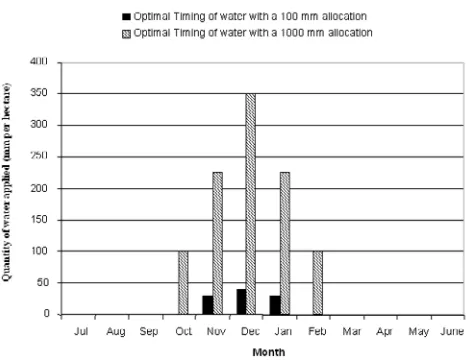
[6] This is because the amount of water actually applied to a crop will depend upon (1) the amount of water available, and (2) the amount, and timing of rainfall during the growing season. To illustrate, assume that grower A has a prepurchased allocation of water which allows him/her to apply up to 1000 mm to the crop over a one year period (from July to June), whereas grower B only has enough to apply 100 mm per hectare. Suppose also, that water is applied ‘‘optimally’’ in the middle of a crop’s life; not much is required early in the crop’s life, and one should not apply water late in season so as to avoid reducing the sugar content of the yield (as illustrated in Figure 1). Finally, suppose that the crop is grown in the tropics, with a typical wet season between October/November and February/March. If the wet season starts early, say in early November, grower B may not end up using any of his/her allocation; grower A might use just 100 mm. If the wet season is late, starting in, say, the end of December, grower B might use 60% of his/her allocation, and grower A might use 67%.

[7] In other words, the amount of water actually applied throughout a season is jointly determined by the amount that is available and by rainfall. Not surprisingly, the amount actually used frequently differs from the amount available for use. Australian Bureau of Agriculture and Resource Economics [1999], for example, provides estimates of the average proportion of allocation used per farm in three regions. These were 83% for Loxton; 92% for Sunraiysia, and 59% for the Murrumbidgee Irrigation Area.

[8] This is somewhat problematic since irrigators are occasionally asked to decide how much water to purchase at the beginning of a season - in the knowledge that any

un-used ‘‘excess’’ cannot be held-over until the next season and hence has no residual value. Decision makers therefore need information about the value of prepurchased or ‘‘allocated’’ water, and it is to this end which the paper is focused.

[9] More specifically, we use an agronomic simulation model to estimate short-run production functions and hence the marginal value of water allocations in different situa-tions. Our production functions differ from those of other researchers since we use the water available for use as the variable factor of production. We call these allocation functions (as opposed to ‘‘traditional’’ production functions, referred to here as irrigation functions, which use the water actually applied as the variable factor of production). They are, nevertheless production functions since they describe the maximum amount that can be produced with different amounts of a variable input (allocation); given technology, given rainfall, given other factors of production, and assum-ing that any ‘‘unused’’ portion of the allocation has no residual value. Unless it is optimal to use all allocations in all years, the two approaches will generate different esti-mates of the marginal value of water. We investigate the implications of that using the following organizational structure:

[10] In section 2, we elaborate on the allocation versus irrigation problem and use results from the simulations to illustrate the potential magnitude of the different ‘‘valua-tions’’ obtained from the different production functions. In section 3, we present simulated results from a small subset of the 56 different allocation functions estimated during our investigations. The primary aim of the analysis is not to generate empirical results for policy, but rather to show how the allocation approach can be used in conjunction with ‘‘real’’ climatic data with ‘‘real’’ soil information and with agronomic models to generate valuable information for irrigators and policy makers, alike. In the concluding section, we discuss the implications of our analysis.

2. Production Functions

[11] That crop yields are not just a function of the amount of water applied, but also of when it is applied is well documented in the literature.Scheierling[1997], for exam-ple, found that for maize ‘‘highest yields often obtained when irrigation water is applied toward the beginning of the season.’’Tilahun and Raes[2002] found that reductions or increases in irrigation will have the largest impact on maize and groundnut yields if timed to coincide with flowering. Zhang and Oweis [1999] similarly found that timing was important for wheat yields and the story is no different for sugarcane which in some conditions responded considerably more to irrigation before canopy closure than after [ Inman-Bamber et al., 1999]. This means that yield response curves (empirically observed relationships between irrigation water and yields) are not analytically equivalent to short-run production functions, because yield-response curves do not, necessarily, describe the maximum yield which can be grown with a given quantity of water.

[12] In theory, one can determine the ‘‘value’’ of irrigation water by estimating a short run production function, from which one can derive a water demand function. Other ways of estimating the value of irrigation water are not considered here. Interested readers are directed to Renwick[2001] and Figure 1. Optimal timing of irrigation with different

Al-Weshah[2000] for examples of the ‘‘residual method.’’ In practice it can be very difficult to estimate the curves from experimental data. One can estimate a yield-response curve for 10 different water allocations, but one cannot guarantee that the curve is an ‘‘optimal’’ one. Consequently, one might need to use 100 different experimental plots (10 different water allocations, each using 10 different irrigation strate-gies). However, then, results may differ from region to region, according to climate, soil type, crop type (etc.). Hence the need for more experimental plots and more research funding. To this end, agronomic models which simulate crop growth offer themselves as a cost-effective alternative.

[13] Nowadays, simulation models are frequently used to examine ‘‘optimal’’ irrigation and water use strategies [see, e.g.,Bergez et al., 2002;Tilahun and Raes, 2002;Kipkorir et al., 2001; Garrido, 2000;Raghuwanshi and Wallender, 1998;Scheierling, 1997]. Although approaches and focuses vary from study to study, most research of this type simulates crop growth under a variety of different irrigation strategies, selecting that which maximizes yield. These relations are analytically equivalent to the ‘‘theoretically correct’’ production functions, since they describe the maximum output which can be had from a given amount of irrigation.

[14] Here we present the output of an agronomic model (APSIM-Sugarcane) that uses real climatic data to generate a set of simulated sugar-cane production functions in seven different regions (using a variety of different soil-types, crop start-dates, etc). APSIM simulates growth of a uniform block of cane. It requires data on soil, crop, weather, and management practices and makes predictions about a range of different variables including: biomass yield and sucrose content (see Keating et al. [1999], Inman-Bamber et al. [1999], and Muchow and Keating [1998] for a detailed description of the way in which APSIM works).

[15] We simulated cane growth in seven different regions using: 41 years of ‘‘real’’ climatic data; 4 different soil-types; 2 different crop-start dates: 10 different irrigation strategies; and 11 different water allocations (i.e., total quantity of water available for use during a 12 month growing season). The irrigation strategies were based on simulated yield loss due to water stress. At one extreme, was a strategy that applied water the day after yield accumulation was suppressed due to water stress. With this strategy water allocations can run out relatively early in the crop’s life and can lead to severe yield loss if rains fail to sustain growth. A strategy at the other extreme, was one which did not irrigate until yield accumulation fell substan-tially. This strategy spread water-use over a longer period. For each region, year, soil, start-date and water allocation, we selected one crop: that with the highest sucrose yield (corresponding to an ‘‘optimal’’ irrigation strategy). By plotting sucrose yield against water allocation (for each year, soil type, region and start-date), we were thus able to derive a set of short-run production functions.

[16] Before proceeding further, we wish to reiterate the difference between allocation production functions and the irrigation production functions typically used by other researchers [e.g., Bergez et al., 2002; Tilahun and Raes, 2002; Kipkorir et al., 2001; Garrido, 2000; Raghuwanshi and Wallender, 1998; Scheierling, 1997]. Allocation

pro-duction functions show the maximum yield for each allo-cation. Irrigation production functions show the maximum yield for each quantity of irrigation used. Unless it is optimal to use all allocations in all years, the different production functions will generate different estimates of the marginal value of water. While absolute differences will vary by crop, region, climate (etc), one expects the gap between estimates to increase as the gap between allocation and actual irrigation increases.

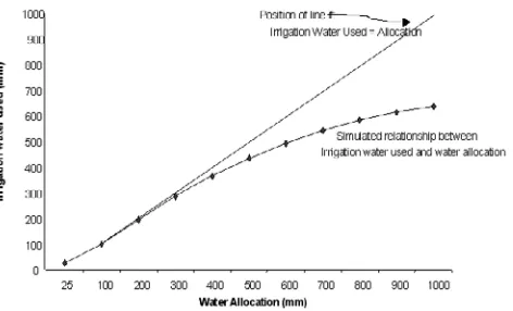
[17] Figure 2 shows the simulated irrigation against water allocation (averaged across all regions, start-days and soil types) for our model runs. At low allocations, the full amount is used because rainfall plus allocation is less than crop requirement. As allocation rises, the proportion used falls to as little as 65% at the highest level; crop require-ments are satisfied by rainfall plus only 65% of the allocation. In one region, for example (Mackay), there were 2460 ‘‘observed’’ values for sucrose yield for each water ‘‘allocation’’ (41 years, for each of 3 different soil types, 2 different crop start dates and 10 different irrigation strategies). At the highest water allocation, only 3 of those 2460 ‘‘observations’’ used all water.

[18] Production functions which optimize on irrigation rather than on allocation, are overvaluing prepurchased water since they implicitly assume that all of the water will be used thereby contributing to production. Clearly, this will not be so in all cases. More formally, short run production functions which use the total water available for irrigation as the variable factor of production (allocation functions) show the increase in sucrose (S) from an increase in water allocations (@S/@A). Short-run production functions which use irrigation as the variable factor of production (irrigation functions) show the increase in sucrose from the increase in irrigation (@S/@I). Hence@S/@A = (@S/@I)(@I/@A) and if@I/ @A is less than one,@S/@A must be less than@S/@I.

[19] A priori, one expects@I/@A to be affected by many factors including: rainfall (wet years using lower propor-tions of allocapropor-tions); climate (wet regions using lower proportion of allocations); soil (better quality soils needing less irrigation and thus a lower proportion of allocation); current allocation levels (the higher the allocation, the lower the proportion used); and perhaps most importantly, on the residual value of any unused allocation (e.g., if the unused portion can be ‘‘carried over’’ until next year, then its value is more appropriately reflected by the irrigation functions). Hence it is difficult to draw generalizations about the

empirical significance of the difference between@S/@A and @S/@I. We can, however, comment on differences for these simulations, assuming that all un-used allocation is ‘‘lost.’’ [20] Figure 3 shows the allocation and irrigation marginal product (MP) curves for the Mareeba region. For any given real price, the irrigation curve overestimates the ‘‘optimal’’ quantity. For example, if the ‘‘real’’ price is (approximately) 1, the allocation MP curve indicates an optimal allocation of approximately 700 mm per hectare, whereas the irrigation curve indicates that 900 mm is more appropriate. From an alternative perspective, irrigators wishing to assess the ‘‘value’’ of water rights, may be enticed into paying too much for allocations if using irrigation curves to estimate the value of extra water. Such an overpayment could be substantial at high allocations.

[21] To illustrate the overvaluation problem mathemati-cally, let us suppose that water allocations must be pre-purchased, that the residual value of an allocation is zero, and that irrigators are risk-neutral, profit maximizers. Irri-gators who use allocation functions to estimate the value of water, will purchase irrigation water as long as it’s real price (PA) is less than or equal to the expected value (EV) of its marginal product (calculated from the allocation functions), i.e., as long as:

PAEVð@S=@AÞ

In contrast, irrigators who use irrigation functions to estimate the value of water will purchase irrigation water as long as its real price (PI) is less than or equal to the expected value (EV) of its marginal product (calculated from the irrigation functions):

PIEVð@S=@IÞ

PIEVð@S=@AÞEVð@A=@IÞ

PIPAEVð@A=@IÞ

If it is not optimal to use all of one’s allocation (i.e., if the EV(@I/@A) < 1), then the EV(@A/@I) > 1, and PI> PA. In other words, those using irrigation functions will be inclined to pay ‘‘too much’’ for their allocations.

[22] This result also extends to the case of risk averse irrigators. To illustrate, note that those requiring compensa-tion for risk may attach a risk ‘‘premium’’ (say, d > 0) to

prices. Those using allocation functions will prepurchase irrigation water as long as its real price (PAR) is less than or equal to PA(1 +d), whereas those using irrigation functions will prepurchase irrigation water as long as its real price (PIR) is less than or equal to:

EVð@S=@IÞð1þdÞ ¼EVð@S=@AÞEVð@A=@IÞð1þdÞ ¼PAREVð@A=@IÞ

While we acknowledge that short-run production functions can be estimated using either water allocations or irrigation, we contend that the allocation functions, are, on occasion, most appropriate. This is so when: growers must pre-purchase water allocations at the beginning of the season; when there is imperfect knowledge about future rainfall; and when un-used amounts have no residual value.

[23] As noted byBond[1998, p. 553] ‘‘Irrigation sched-uling in practice is far less precise than in design models, and rain interruptions, irrigation failures, spatial variability of irrigation rates, and other operational difficulties mean that irrigation is unlikely to be applied as prescribed.’’ Unless one can forecast rainfall perfectly, production func-tions which relate yield to irrigation cannot accurately estimate the value of prepurchased allocations; they are really just ex-post descriptions of what could have been grown with ‘‘x’’ mm of water (and ‘‘y’’ mm of rain).

3. Allocation Production Functions as an Information Source

[24] Before proceeding it is worth noting that our simu-lations allowed us to estimate 56 different production functions (across 7 regions, using 4 different soil types and 2 different crop-start dates). This discussion only focuses on a small selection of those (details of other production functions available on request). Its primary aim is not to generate empirical results for policy, but rather to show how the allocation approach can be used in conjunction with ‘‘real’’ climatic data with ‘‘real’’ soil information and with agronomic models to generate valu-able information for irrigators and policy makers, alike.

[25] The allocation functions are particularly useful when considering irrigation strategies in areas of high rainfall variability. Figure 4 shows two allocation production func-Figure 3. The marginal product of sucrose in Mareeba.

tions for each of the Mackay and Maryborough regions. The functions are averaged across soil types and start-days, but differentiated by rainfall. As expected, at low allocations, dry years show substantially lower yields than wet ones, and the differences between yields fall as water allocations rise. [26] When rainfall is in the upper quartile, and water allocations are low, simulated sucrose yields in Mackay and Maryborough are relatively close. However, large differ-ences are evident when rainfall is in the lower quartile, particularly, at low allocations. This reflects different rain-fall patterns. In Mackay, for example, mean rainrain-fall from 1 July to 30 June during the years considered in these simulations was 1685 mm. In Maryborough, mean rainfall for the same period was only 1084 mm: less than the lower quartile (of 1228 mm) in Mackay. Consequently, variations in rainfall impact upon Maryborough’s cane yields more significantly than on Mackay’s. The message is reinforced by Figure 4.

[27] Figure 5, which shows the MP of Water Allocations for wet and dry years in Maryborough and Mackay. As expected: the marginal product of water allocations in dry years is considerably higher than in wet years; the MPs are similar in wet years; but the MPs differ significantly in dry years (the drier region having much higher valuations).

[28] Evidently, year-to-year variations in rainfall gener-ate much more significant variations in crop yields in some regions than in others. There may also be substantial cross-regional variations in the ‘‘value’’ of irrigation water. In dry years, for example, an increase in water allocation from 400 to 500 mm/ha, is ‘‘worth’’ almost twice as much in Maryborough as it is in Mackay. These two regions do not compete for the same water, but if they did, a transfer of water resources from one area to another could generate a significant pareto improvement. In the Murray Darling Basin, where there is much cross-region competition for water resources, the allocation production function ap-proach suggested in this paper may have much to contrib-ute to policy. Similarly, cross-regional comparisons of the ‘‘value’’ of extra water allocations may assist companies with properties in many regions determine where best to invest in irrigation infrastructure.

[29] These production functions also provide valuable information on an intraregional scale. Figure 6 shows the MP of extra allocations in the Burdekin and at Rocky Point, for ‘‘early’’ and ‘‘late’’ crops. At high allocations, there is

little difference, but at low allocations, late crops derive greater benefit from increased allocations than early crops, irrespective of region. These simulations confirm a priori expectations that an ‘‘even quantity of water across all paddocks’’ strategy is not optimal in all cases. When water resources are scarce, it may be best to irrigate late crops before the early ones [Brennan et al., 1999].

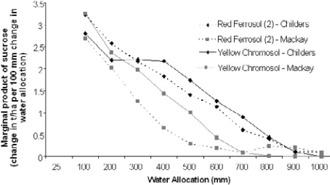
[30] Crops grown on different soil types also respond differently to irrigation. Figure 7 shows the MP of extra water allocations in Mackay and Childers for two different soil-types. That there are regional and soil-type differences is not surprising, but some of the interactive effects were not expected. For example, MP of water allocations for crops grown in Yellow Chromosol is generally higher than the MP of crops grown in Red Ferrosol. Yet the differences are greater in Mackay than in Childers. This indicates that growers in the Mackay region may have more to gain by reallocating irrigation across soil-types than growers in Childers.

4. Discussion

[31] In Australia, current water policy uses a range of ‘‘interlinked market based measures involving pricing water for full cost recovery, establishing secure access to water separate from land, and providing for permanent trading in water entitlements’’ [Department of Primary Industry and Energy, 1999, p. 5]. Such market based measures are popular among current policy makers, at least partially Figure 5. The marginal product of water allocations

(averaged across all soil types and start days).

Figure 6. Marginal products for different start days in the Burdekin and at Rocky Point.

because they are believed to be capable of achieving ‘‘optimal’’ water distributions. Yet for this to occur, ‘‘play-ers’’ in the water market, need quality information, and as noted by Environment Australia [2002, p. 3], ‘‘there is a lack of reliable data available to assist with the character-ization of the extent, location, value and efficiency gains in irrigation management.’’ As in many other markets, inade-quate information, constrains efficiency in water markets [Bjornlund and McKay, 1996].

[32] Advances in computer technology mean that agro-nomic modeling supported by field experimentation is a cost-effective means of generating quality information. Admittedly, one could criticize the modeling approach on the grounds that it simplifies and abstracts from reality. But the abstraction allows one to focus on a sub-set of functions and variables, identifying relationships that might otherwise be hidden within ‘‘real world’’ complexities. And because one can repeat the simulations, altering just one variable (or coefficient) at a time, one can conduct experiments. Experi-ments capable of investigating the impact of almost any ‘‘x’’ on almost any ‘‘y’’; within a ‘‘computerized test-tube.’’ In some sense, therefore, its abstractions are its strength.

[33] This does not mean that the agronomic model used here is perfect. The model does not accurately simulate crop growth in all cases - not because the model is deficient in capturing knowledge about crop growth, but because knowledge per se is deficient. The model is, nevertheless, a particularly good support tool for policy and management decisions because it integrates some of the best information and knowledge available for making these decisions. One should probably not place too much store on the cardinal numbers presented, but the ordinal rankings and qualitative conclusions are, we believe, robust.

[34] More generally, the modeling approach may help with policy formation. One can, for example, use the model to compare the yields of different irrigation strategies (e.g., evenly spread versus optimally timed) thereby estimating the potential gains from improved water-use efficiency. One could also use these kinds of models for a range of different strategies across a range of different policy variables (water, fertilizer, pesticide use, etc), generating ordinal (if not cardinal) estimates of the effect of such strategies on final outputs such as yield, or run-off.

[35] Agronomic models can be also be used to compare the ‘‘value’’ of extra allocations across regions, crop-start-dates, and soil-types. This allows one to identify regions most likely to be affected by drought and cases where profits (and/or social welfare) can be increased by reallocating scarce water resources across regions, crops, or paddocks. This will be particularly important for long-term planning, when using the allocation functions. In the Murray Darling, for example, the price of temporary water will vary, optimally, according to short-run variations in rainfall. However, the market for ‘‘permanent’’ water is a forward looking one and the information requirements of those trading in that market are similar to those who must assess the worth of extra dams, of water storage facilities [e.g.,Smith and Maheshwari, 2002], of extra irrigation channels, etc.

[36] Finally, this simulation approach has allowed us demonstrate (and quantify) the effect which imperfect information vis-a`-vis rainfall has upon the ‘‘value’’ of allocations relative to the ‘‘value’’ of water actually applied.

If it not optimal to use all of one’s allocation, and if the residual value of any unused allocation is zero, then irrigation functions will overestimate the marginal value of extra water allocations, possibly by orders of magnitude. In the Queensland sugarcane industry, irrigators do not generally use all of their allocations. As noted in the introduction, this is also true of irrigators in the Murray Darling; and the situation most likely arises in other places (using ‘‘allocations’’) throughout the world.

[37] Dinar [1998, p. 379], argues that the problem of excessive water use is exacerbated by imperfect information vis-a`-vis: privately observed individual water intakes and water production technologies. To that we add the issue of unknowable future rains (an extreme form of asymmetric information), suggesting that our methodological approach to estimating allocation production functions provides researchers with a means of estimating the empirical mag-nitude of the problem in a broad range of situations.

[38] Acknowledgments. The authors would like to thank the Sugar Research and Development Corporation, the Sugar CRC and the Queens-land Department of Natural Resources and Mines for providing funding for this research. We would also like to thank our (internal) CSIRO referees for their comments and suggestions.

References

Akerlof, G. A., The market for ‘‘lemons’’: Quality uncertainty and the market mechanism,Q. J. Econ.,84, 488 – 500, 1970.

Al-Weshah, R. A., Optimal use of irrigation water in the Jordan Valley: A case study,Water Resour. Manage.,14(5), 327 – 338, 2000.

Australian Bureau of Agriculture and Resource Economics, Irrigation water reforms: Impact on horticulture farms in the southern Murray Darling Basin,ABARE Curr. Issues 99(2), Canberra, 1999.

Bergez, J.-E., J.-M. Deumier, B. Lacroix, P. Leroy, and D. Wallach, Improving irrigation schedules by using a biophysical and a decisional model,Eur. J. Agron.,16(2), 123 – 135, 2002.

Bjornlund, H., and J. McKay, Transferable water entitlements: Early lessons from South Australia,Water,23(5), 39 – 43, 1996.

Bond, W. J., Effluent irrigation—An environmental challenge for soil science,Aust. J. Soil Res.,36(4), 543 – 556, 1998.

Brennan, L. E., S. N. Lisson, N. G. Inman-Bamber, and A. I. Linedale, Most profitable use of irrigation supplies: A case study of the Bundaberg district, paper presented at 21st Conference of the Australian Society of Sugar Cane Technologists, Aust. Soc. of Sugar Cane Technol., Towns-ville, Queensland, Australia, 1999.

Department of Primary Industry and Energy, Progress in implementation of the COAG Water Reform Framework,Occasional Pap. 1, High-level Steering Groups on Water, Brisbane, Queensland, Australia, 1999. (Available at http://www.dpie.gov.au/content/output.cfm?ObjectID= D2C48F86-BA1A-11A1-A2200060B0A05637)

Dinar, A., Water policy reforms: Information needs and implementation obstacles,Water Policy,1(4), 367 – 382, 1998.

Environment Australia, Australian Natural Resources Atlas, version 2, Audit Off. of Environ. Aust., Canberra, 2002. (Available at http://audit. ea.gov.au/anra/)

Garrido, A., A mathematical programming model applied to the study of water markets within the Spanish agricultural sector,Ann. Oper. Res.,95, 105 – 123, 2000.

Inman-Bamber, N. G., M. J. Robertson, R. C. Muchow, A. W. Wood, R. Pace, and A. M. F. Spillman, Boosting yields with limited irrigation water, paper presented at 21st Conference of the Australian Society of Sugar Cane Technologists, Aust. Soc. of Sugar Cane Technol., Towns-ville, Queensland, Australia, 1999.

Keating, B. A., M. J. Roberston, R. C. Muchow, and N. I. Huth, Modelling sugarcane production systems. I. Description and validation of the APSIM Sugarcane module,Field Crops Res.,61, 253 – 271, 1999. Kilgour, D. M., and A. Dinar, Flexible water sharing within an international

river basin,Environ. Resour. Econ.,18(1), 43 – 60, 2001.

Kipkorir, E. C., D. Raes, and J. Labadie, Optimal allocation of short-term irrigation supply,Irrig. Drainage Syst.,15(3), 247 – 267, 2001. Lenzen, M., and B. Foran, An input-output analysis of Australian water

Mackie-Mason, J. K., J. F. Riveros, M. S. Bonn, and W. P. Lougee, A report on the PEAK Experiment: Usage and economic behaviour,D-Lib Mag., 5(7)/(8), doi:10.1045/july99-mackie-mason, 1999.

Meinzen-Dick, R. S., and W. van der Hoek, Multiple uses of water in irrigated areas,Irrig. Drainage Syst.,15(2), 93 – 98, 2001.

Muchow, R. C., and B. A. Keating, Assessing irrigation requirements in the Ord Sugar Industry using a simulation modelling approach,Aust. J. Exp. Agric.,38(4), 345 – 354, 1998.

Pigram, J., Tradeable water rights: The Australian experience, Cent. for Water Policy Res., Armidale, New South Wales, Australia, 1999. Raghuwanshi, N. S., and W. W. Wallender, Optimal furrow irrigation

scheduling under heterogeneous conditions,Agric. Syst.,58(1), 39 – 55, 1998.

Renwick, M. E., Valuing water in a multiple-use system—Irrigated agriculture and reservoir fisheries,Irrig. Drainage Syst.,15(2), 149 – 171, 2001.

Scheierling, S. M., Impact of irrigation timing on simulated water-crop production functions,Irrig. Sci.,18(1), 23 – 31, 1997.

Smith, A., and B. L. Maheshwari, Options for alternative irrigation water supplies in the Murray-Darling Basin, Australia: A case study of the

Shepparton Irrigation Region,Agric. Water Manage., 56(1), 41 – 55, 2002.

Tilahun, K., and D. Raes, Sensitivity analysis of optimal irrigation sche-duling using a dynamic programming model, Aust. J. Agric. Res., 53(3), 339 – 346, 2002.

Varela-Ortega, C., M. Sumpsi, J. Garrido, and A. Blanco, Water pricing policies, public decision making and farmers’ response: Implications for water policy,Agric. Econ.,19(1 – 2), 193 – 202, 1998.

Wichelns, D., An economic model of waterlogging and salinization in arid regions,Ecol. Econ.,30(3), 475 – 491, 1999.

Zhang, H., and T. Oweis, Water-yield relations and optimal irrigation scheduling of wheat in the Mediterranean region,Agric. Water Manage., 38(3), 195 – 211, 1999.

N. G. Inman-Bamber, Davies Laboratory, CSIRO Sustainable Ecosystems, Private Mail Bag, Aitkenvale, Queensland 4814, Australia.