Algorithmic Framework and Implementation of Spectrum Holes Detection for Cognitive Radios

Theses Thesis/Dissertation Collections

5-2017

Algorithmic Framework and Implementation of

Spectrum Holes Detection for Cognitive Radios

Ian J. Frasch

[email protected]

Follow this and additional works at:http://scholarworks.rit.edu/theses

This Thesis is brought to you for free and open access by the Thesis/Dissertation Collections at RIT Scholar Works. It has been accepted for inclusion in Theses by an authorized administrator of RIT Scholar Works. For more information, please [email protected].

Recommended Citation

Implementation of Spectrum Holes

Detection for Cognitive Radios

by

Ian J. Frasch

A Thesis Submitted in Partial Fulfillment of the Requirements for the Degree of Master of Science

in Computer Engineering

Supervised by

Dr. Andres Kwasinski

Department of Computer Engineering Kate Gleason College of Engineering

Rochester Institute of Technology Rochester, New York

May 2017

Approved by:

Dr. Andres Kwasinski

Thesis Advisor, Department of Computer Engineering

Dr. Panos Markopoulos

Committee Member, Department of Electrical Engineering

Dr. Marcin Lukowiak

Abstract

Algorithmic Framework and Implementation of Spectrum Holes Detection for Cognitive Radios

Ian J. Frasch

Contents

Abstract . . . ii

Acronyms . . . ix

1 Introduction. . . 1

1.1 Cognitive Radio . . . 2

1.1.1 Regulatory Compliance . . . 3

1.1.2 Potential Applications . . . 3

1.1.3 Current State . . . 4

1.2 Contribution of Thesis . . . 4

2 Background . . . 6

2.1 Energy Detection . . . 6

2.1.1 Advantages . . . 7

2.1.2 Drawbacks . . . 8

2.2 Cyclostationary Detection . . . 8

2.2.1 Spectral Correlation Density (SCD) . . . 8

2.2.2 Spectral Coherence . . . 9

2.2.3 Gallery of Spectral Coherence . . . 10

2.2.4 Existing Work . . . 11

2.2.5 Advantages . . . 12

2.2.6 Drawbacks . . . 13

2.3 Detector Performance Metrics . . . 13

3 Detection Algorithm . . . 15

3.2 Single-Band Cyclostationary Detection Algorithm . . . 16

3.3 Simulation of Single-Band Algorithms . . . 18

3.3.1 Setup . . . 18

3.3.2 Results . . . 20

3.3.3 Conclusion . . . 21

3.4 Multiband Detection Algorithm . . . 22

3.5 Simulation of Multiband Algorithm . . . 24

3.5.1 Results . . . 24

3.5.2 Remarks for Implementation . . . 25

4 Implementation . . . 27

4.1 SDR Platform . . . 27

4.2 Implementation Overview . . . 28

4.3 Implementation Architecture . . . 30

4.3.1 Hardware datapath . . . 31

4.3.2 Nios software . . . 31

4.3.3 PC interface . . . 31

4.4 Details . . . 32

4.4.1 Design . . . 32

4.4.2 DC Offset Handling . . . 32

4.4.3 Fixed-point Bit Growth . . . 33

4.4.4 Antenna and Frequency Considerations . . . 33

4.5 Resource Utilization . . . 34

4.6 Requirements for Implementation . . . 34

4.7 Source Code . . . 35

5 Experiments and Results . . . 36

5.1 Implementation Issues . . . 36

5.1.2 Analog Filter Frequency Response . . . 37

5.2 Side Experiment: Noise Characterization . . . 37

5.2.1 Noise Floor Variation . . . 37

5.2.2 PSD and Spectral Coherence of Noise . . . 38

5.3 Setup of Performance Experiments . . . 39

5.3.1 Detector Parameters and Characteristics . . . 40

5.4 Results . . . 41

5.4.1 Single Transmission . . . 41

5.4.2 Multiple Transmissions . . . 43

5.4.3 Example Detector Output . . . 43

6 Conclusion . . . 45

List of Tables

3.1 Setup of QPSK and OFDM Test Signals . . . 18

4.1 Implementation Specifications and Settings . . . 30

4.2 FPGA Resource Utilization of Hole Detector . . . 34

List of Figures

1.1 Dynamic discovery of spectrum holes [1] . . . 1

1.2 IEEE 802.22 Wireless Regional Area Network (WRAN) cell

with base station and user terminals [2]. . . 3

2.1 PSD and spectral coherence estimates of 4-FSK signal at

SNR = 5 dB. . . 10

2.2 PSD and spectral coherence estimates of 16-QAM signal at

SNR = 15 dB. . . 11

2.3 PSD and spectral coherence estimates of 16-QAM signal at

SNR = -5 dB. . . 11

2.4 PSD and spectral coherence estimates of white Gaussian

noise. . . 11

3.1 PSD and spectral coherence of 9216-sample QPSK test

sig-nal at SNR = 15dB (Fs is the sampling frequency). . . 19

3.2 PSD and spectral coherence of 9216-sample OFDM test

sig-nal at SNR = 15dB (Fs is the sampling frequency). . . 19

3.3 PSD and spectral coherence of 9216-sample QPSK test

sig-nal at SNR = -5dB (Fs is the sampling frequency). . . 20

3.4 Probability of Detection vs SNR with fixed PF A=0.1 for (a)

QPSK test signal and (b) OFDM test signal. . . 20

3.5 Detector ROC curves with fixed SNR for (a) QPSK test

sig-nal with SNR = -10 dB and (b) OFDM test sigsig-nal with SNR

3.6 Performance of multiband energy detection algorithm. (a)

Average percentage of signal power detected in signal’s

band-width vs in-band SNR (b) Probability of detecting at least

90% of the power in signal’s bandwidth vs in-band SNR . . 25

3.7 Effects on detection performance (a) increased sensing time

(and therefore number of FFT averages) and (b) decreased

FFT size. . . 25

4.1 Block diagram of receive chain in the bladeRF

implementa-tion platform . . . 27

4.2 Image of bladeRF device . . . 28

4.3 Method of operation for scanning wide bandwidth: example

with 3 frequencies. Illustrates the sensing time (per band),

retune time, and instantaneous bandwidth of the receiverBWI 29

4.4 Implementation Architecture . . . 30

5.1 PSD and spectral coherence estimates of real noise received

with the bladeRF . . . 38

5.2 Experimental Setup . . . 39

5.3 Detector performance for a single continuous transmission

and fixed PF A = 0.09 . . . 42

5.4 Detector ROC curve for a single continuous transmission

and fixed in-band SNR = -6 dB . . . 42

5.5 Detector performance for three continuous transmissions . . 43

5.6 Real-time output from the detector with three wired QPSK

transmissions with bandwidths of 5 MHz. (a) Scaled power

spectral density; (b) Detected holes; (c) Rankings of

Acronyms

ADC Analog to Digital Converter

AWGN Additive White Gaussian Noise

CD Cyclostationary Detection

DAC Digital to Analog Converter

DC Direct Current

ED Energy Detection

FFT Fast Fourier Transform

FPGA Field Programmable Gate Array

GPIF General Programmable Interface

IQ In-phase/Quadrature

OFDM Orthogonal Frequency Division Multiplexing

PD Probability of Detection

PFA Probability of False Alarm

PSD Power Spectral Density

PSK Phase Shift Keying

QAM Quadrature Amplitude Modulation

RF Radio Frequency

SC Spectral Coherence

SCD Spectral Correlation Density

SDR Software-Defined Radio

SMA SubMiniature version A

SNR Signal to Noise Ratio

SPI Serial Peripheral Interface

UART Universal Asynchronous Receiver/Transmitter

Chapter 1

Introduction

The ability to dynamically discover portions of unused radio spectrum (holes) and utilize those holes leads to wireless communication which is faster, more reliable, and more efficiently uses the spectrum. Dynamic sensing of the spectrum can reduce interference, which is especially important in the present day world which is filled with wireless communication systems con-stantly transmitting. Dynamic spectrum access (DSA) refers to dynamically switching operating frequency and/or bandwidth to use available spectrum holes. The concept of dynamic spectrum access is illustrated in Figure 1.1. Regulation of the radio spectrum has caused an apparent spectrum scarcity, which is challenging for the launch of new wireless services such as 5G cellular networks. However, this scarcity is an artificial limitation since significant portions of licensed spectrum are unoccupied most of the time. Systems are needed which can employ dynamic spectrum access to utilize spectrum holes, overcoming the problem of spectrum scarcity.

1.1

Cognitive Radio

Cognitive radio refers to an emerging field of intelligent wireless commu-nication systems which adapt their transmission/reception parameters based on the environment. A cognitive radio is meant to be aware of its environ-ment, producing reliable communication whenever and wherever needed and efficiently use the radio spectrum. In addition to spectrum sensing for dynamic spectrum access, cognitive radios employ channel estimation and transmit power control to reduce interference with other radios. Based on changes in input stimuli, cognitive radios adapt communication parameters such as carrier frequency, bandwidth, modulation scheme or strategy, and transmit power. Decisions are made using learning and reasoning. The primary goal of cognitive radio is to dynamically share the spectrum for efficient spectrum use, eliminating spectrum scarcity. Cognitive radio is built on software-defined radio (SDR), a flexible and reconfigurable radio platform which is commercially available today. The detection of spectrum holes is a defining ability of a cognitive radio system, allowing it to find vacant frequency bands and avoid interfering with other users [3].

A cognitive radio contrasts with traditional radios which use a fixed por-tion of allocated spectrum and contain fixed funcpor-tionality hardware. When a traditional radio is not transmitting, the spectrum it has been licensed to use is wasted since it cannot be used by anyone else. Cognitive radios are meant to reduce this wasted spectrum by dynamically sharing the spectrum; lead-ing to more efficient overall spectrum use. The spectrum can be shared both with licensed transmitters (primary users) and with other cognitive radios (secondary users) .

1.1.1 Regulatory Compliance

In the United States, large portions of spectrum inside the 54 MHz - 862 MHz region were made available when the Federal Communications Com-mission (FCC) ordered the termination of analog television transCom-mission in the 2009 digital switchover mandate. The FCC has authorized unlicensed transmitters to use these frequencies, also known as white spaces, provided they do not interfere with a licensed service [4]. This provides legal oppor-tunity for cognitive radios to thrive. In the future more areas of the spectrum may be opened up to unlicensed cognitive transmitters, allowing more op-portunity for communication.

1.1.2 Potential Applications

Cognitive radio networks have been standardized in IEEE 802.22: Wireless Regional Area Networks (2011). This standard outlines specifications for cognitive radio networks which operate in TV bands between 54 MHz and 862 MHz, sharing spectrum with licensed TV broadcasters [2]. The stan-dard envisions a wireless network employed in rural locations to provide broadband internet access, illustrated in Figure 1.2.

1.1.3 Current State

Theoretical research on cognitive radio is abundant, software-defined radios are commercially available, white space frequencies are legally available, and there is even an IEEE standard, but cognitive radios are still not yet out of the laboratory for everyday commercial use. It seems that the missing piece of the puzzle is implementation. Implementation-focused research can help make the vision of cognitive radios a reality.

1.2

Contribution of Thesis

This thesis is focused on implementation of the spectrum hole detection ability of cognitive radios. Existing research covers theoretical methods of sensing the radio spectrum and detecting holes/signals, but lacks content on implementations (especially wideband implementations) and implementa-tion issues. Existing research also tends to lack algorithms that could real-istically be implemented to scan a gigahertz-order range of frequencies to blindly detect signals. Implementation feasibility of algorithms is typically not discussed.

Chapter 2

Background

Spectrum hole detectors for cognitive radios detect the presence of trans-mission signals across a wide range of frequencies and assert that holes exist in frequencies where signals are absent. Typically detection must be performed without any a-priori knowledge of the signals to be detected. This type of detection is referred to as blind detection. Matched filter de-tection is considered the optimum technique for signal dede-tection [5], but is not discussed in this thesis because it is a non-blind technique which re-quires complete knowledge of the signals to be detected. The two primary techniques for blind spectrum hole detection are energy detection and cy-clostationary feature detection [6]. Energy detection is the most common and straightforward approach; it refers to observing the spectral energy (or power) at different frequencies and using a threshold to decide if a signal is present at each frequency. The potential problem with energy detection is that it requires accurate estimation of the spectral noise floor in order to choose the detection threshold. Cyclostationary feature detection refers to taking advantage of the innate spectral correlation that exists in transmis-sion signals and not in noise. Cyclostationary feature detection typically involves extraction of peaks or features in the computed spectral correlation density.

2.1

Energy Detection

truncated Fourier transform, as shown in equation 2.1.

Sxx(f) = lim T→∞

E[|XT(f)|2]

T (2.1)

where E[·] is the expectation operator and XT(f) is the truncated Fourier

transform of the input time-domain signal x(t):

XT(f) = T /2

Z

−T /2

x(t)e−j2πf tdt (2.2)

To determine if a signal is present, the PSD values are compared to the detection threshold which is set based on the noise power. In frequencies where the PSD value exceeds the threshold, the energy detector asserts that a signal is present:

Sxx(f) ≥ T hreshold : signal present (2.3)

Energy detection algorithms for cognitive radios are proposed in [7] and [8]. For best performance in practice, energy detectors should use the highest number of Fourier transform averages possible. Increasing the number of averages will produce a more accurate PSD estimate at the cost of a longer sensing time (meaning longer signal length). As the number of averages is increased, the PSD estimate of white Gaussian noise approaches a flat horizontal line.

2.1.1 Advantages

2.1.2 Drawbacks

An inaccurate estimate of in-band noise power can reduce performance from the energy detector. For example, if the noise power estimate is too high, the chosen detection threshold will be higher, causing a decreased probability of signal detection. The work in [9] and [10] quantifies the effect of uncertain noise power estimates on performance of energy detectors. Noise power estimation can be difficult in practice, especially since (1) the power of noise generated by RF front ends can vary over frequency, (2) the noise floor can also consist of external (background) noise in addition to thermal noise, and (3) thermal noise power varies over temperature.

2.2

Cyclostationary Detection

A cyclostationary signal is defined as a random process with periodic mean and autocorrelation. Cyclostationarity causes spectral correlation: meaning the magnitude and phase of different frequency components of the signal are correlated over time. The spectral correlation between different frequencies is given by the spectral correlation density (SCD). Cyclostationary detection identifies signals by looking for peaks or shapes in the computed SCD or spectral coherence (a normalized version of the SCD). Stationary noise does not exhibit spectral correlation, and therefore its theoretical SCD would be zero.

2.2.1 Spectral Correlation Density (SCD)

the power spectral density. Formally, the SCD is given by

S_xα(f) = lim

T→∞∆limt→∞

1 ∆t

∆t/2

Z

−∆t/2

1

TXT(t, f +α/2)X ∗

T(t, f −α/2)dt (2.4)

where XT is the finite-time Fourier transform of the the input time-domain

signal x(u); representing the Fourier transform over time:

XT(t, f) =

t+T /2

Z

t−T /2

x(u)e−j2πf udu (2.5)

2.2.2 Spectral Coherence

Spectral coherence is a useful detection statistic derived from the SCD. Spectral coherence is a normalized version of the SCD which ranges be-tween 0 and 1 in magnitude. It is essentially the correlation coefficient for the SCD. Spectral coherence is given by

C_xα(f) = S

α x(f)

p S0

x(f +α/2)Sx0(f −α/2)

(2.6)

whereS_xα(f)is the spectral correlation density, with parameterα.

Conceptually, the spectral coherence represents the correlation between two frequency components located at(f +α/2)and(f −α/2)normalized by the PSD at each frequency.

mean magnitude regardless of the noise power. This means that no noise power estimate is needed. The spectral coherence magnitude of a signal only depends on its SNR. This lends the ability to set a fixed detection threshold without having to worry about changing noise levels or changing gain.

2.2.3 Gallery of Spectral Coherence

Figures 2.1, 2.2, 2.3, and 2.4 show examples of spectral coherence estimates computed in MATLAB, along with corresponding PSD estimates. The spec-tral coherence corresponding to α = 0 has been omitted since it is always equal to 1. Each input signal had a length of 9216 samples. Root-raised co-sine pulse shaping was applied to the 16-QAM signal. The 16-QAM signal was modulated at 4 samples per symbol, and the 4-FSK signal was modu-lated at 16 samples per symbol. Distinct features are clearly visible in the spectral coherence of the signals at high SNR, shown in Figures 2.1 and 2.2. Observe in Figure 2.3 that the features in the spectral coherence of the 16-QAM signal are diminished in low SNR. Observe that in Figure 2.4 the the magnitude of the spectral coherence estimate of white Gaussian noise is slightly above zero. This is due to the finite signal length of 9216 samples. A longer signal length would produce more accurate spectral coherence es-timate at the cost of a longer sensing time in practice. As the signal length is increased, the spectral coherence estimate of noise approaches zero, and the PSD estimate of noise approaches a flat horizontal line.

Figure 2.2: PSD and spectral coherence estimates of 16-QAM signal at SNR = 15 dB.

Figure 2.3: PSD and spectral coherence estimates of 16-QAM signal at SNR = -5 dB.

Figure 2.4: PSD and spectral coherence estimates of white Gaussian noise.

2.2.4 Existing Work

about the signals to be detected. Non-blind techniques are not useful for the general purpose spectrum sensing needed by cognitive radios. Existing work in blind detection algorithms includes the work in [11], which uses the squared magnitude of the spectral coherence as a detection statistic, then uses a threshold test to determine if a signal is present:

|C_xα(f)|2 ≥ T hreshold : signal present (2.7)

For blind detection, the work in [12] suggests using the crest factor of the

α-domain profile as a detection statistic, where theα-domain profileI(α)is defined as the maximum observed C_xα(f) magnitude for each α. The crest factor (CF) is defined as the ratio of peak amplitude to root-mean-square amplitude:

I(α) =∆ max

f |C α

x(f)| (2.8)

CF(I(α)) ≥ T hreshold : signal present (2.9)

For non-blind detection, the work in [13] suggests integrating the SCD over a ”feature mask” to detect signals, where the feature mask restricts the in-tegration to the range of values for (α, f) values where peaks/features are expected. This requires the receiver to know a-priori the frequency and theoretical SCD of the input signal, and therefore cannot be used for blind detection.

Research in [14] and [15] suggests using cyclostationary detection for fine sensing (with a long sensing time) and energy detection algorithms for coarse sensing (with a short sensing time).

2.2.5 Advantages

2.2.6 Drawbacks

Cyclostationary detection is thought of as the more robust technique by many researchers since noise does not exhibit spectral correlation (SCD is zero). However this only applies to the ”true” SCD which in theory in-volves sensing for an infinite amount of time. Practical estimates of the SCD use a finite sensing time causing the SCD estimate for noise to be small but not zero (as shown in Section 2.2.3). Increased sensing time in-creases performance of cyclostationary detection but also inin-creases perfor-mance of energy detection, since more Fourier transform averages produce a flatter noise spectrum. Existing research has shown that cyclostationary fea-ture detection requires longer sensing time to achieve the same performance as energy detection [13]. As mentioned in Section 2.2.4, some cyclosta-tionary detection algorithms require a-priori knowledge of the signals to be detected, which is not useful for blind detection. Additionally, the entire bandwidth of a signal must be captured in order for spectral correlation to be seen. Partially captured signals may not exhibit any spectral correlation. For example, if the receiver’s bandwidth only covers half of the bandwidth of a signal, spectral correlation features may be completely nonexistant in the SCD estimate. Computation of the SCD also involves higher computa-tional complexity leading to increased use of hardware/software resources in implementation.

2.3

Detector Performance Metrics

The common metrics to characterize the performance of a signal detector are the probability of detection (PD) and the probability of false alarm (PF A).

PD is the probability of correctly detecting a signal; in other words, the

prob-ability for the system to detect a signal when in reality a signal is present.

PF A is the probability of incorrectly detecting a signal; in other words, the

probability for the system to detect a signal when in reality no signal is present. A related metric is the required SNR for a certain PD, which is the

minimum SNR required to correctly detect a signal with probability PD.

The higher the value of PF A, the more available spectrum opportunities are

missed. The value of PD depends only on the received SNR. The lower the

value of PD, the more likely it is to interfere with primary users or other

secondary users. The IEEE 802.22 standard for cognitive radio networks specifies that PF A should be less than or equal to 0.1 and PD should be

greater than or equal to 0.9 [2]. The two metrics oppose each other; chang-ing the detection threshold(s) to increasePD will also increase PF A.

Another performance metric of interest is the sensing time required to meet a particular PD and PF A for a given SNR. Increasing the sensing time

Chapter 3

Detection Algorithm

This chapter compares single-band energy detection and cyclostationary de-tection algorithms for signal dede-tection, then selects the better of the two and modifies it for multiband detection. Both considered single-band algorithms require no a-priori knowledge of the noise power, and use a simple threshold test to determine if a signal is present. The performance of both algorithms is compared through MATLAB simulations with a single signal affected by additive white Gaussian noise (AWGN). It will be seen that the energy detection algorithm yields better performance.

3.1

Single-Band Energy Detection Algorithm

The proposed single-band energy detection (ED) algorithm detects the pres-ence of a signal using a power spectral density (PSD) estimate and does not require a-priori knowledge of the noise power. The noise power is instead estimated as the minimum value of the PSD. The basis of this estimate is the assumption that at least one frequency bin is unoccupied by signals during the sensing time. This is expected to hold true in implementations where the receiver bandwidth is large enough that typical transmissions would not occupy the entire band. The target implementation platform can receive 28 MHz of RF bandwidth, which was deemed to be wide enough to support this algorithm. This is because 28 MHz is wide enough to cover typical transmissions, including 20 MHz Wi-Fi transmissions and 6-8 MHz digi-tal TV transmissions. Performance of this algorithm would be significantly reduced in situations where the entire observable band of frequencies is oc-cupied by signals, as it would result in a poor noise estimate. The algorithm is described as follows:

no windowing functions or overlap between FFTs.

X[k] = NF−1

X

n=0

x[n]·e−j2π

k

NFn _(3.1)

2. Compute the power spectral density (PSD) using the average squared magnitude of the FFTs.

Sxx[k] =

E[|X[k]|2_]

NF

(3.2)

3. Find the minimum PSD value and use it as an estimate of the noise floor.

4. Set the detection threshold T hED to be the minimum PSD value

mul-tiplied by fixed scaling factorSF.

T hED = min{Sxx[k]} ·SF (3.3)

5. If the maximum value of the PSD is greater or equal to T hED, assert

that a signal is present.

max{Sxx[k]} ≥ T hED : signal present (3.4)

The scaling factor SF is chosen based on the desiredPF A. Finding the SF

that corresponds to a specific PF A requires simulation of the detector with

an input vector of pure noise; varying the SF until it produces the desired

PF A. Note that selection ofSF does not depend on received noise power.

3.2

Single-Band Cyclostationary Detection Algorithm

1. Compute successive NF-point FFTs of the input signal over time with

no windowing functions or overlap between FFTs.

XNF[n, f] (3.5)

2. Compute the scaled PSD using the summed squared magnitude of the FFTs. (Note: N refers to the number of successive FFTs computed).

˜

Sxx[f] = N−1

X

n=0

|XNF[n, f]|

2 _(3.6)

3. Compute spectral correlation density (SCD) by calculating the com-plex dot product between FFT frequency-over-time vectors at bins(f+

α/2)and (f −α/2).

˜

Sα x[f] =

N−1

X

n=0

XNF[n, f + α/2]X

∗

NF[n, f −α/2] (3.7)

4. Compute the squared magnitude of the spectral coherence by divid-ing the squared magnitude of each SCD value by the product between PSD(f + α/2)and PSD(f −α/2).

|C˜α x[f]|

2 ₌ |S˜xα[f]|2 ˜

Sxx[f + α/2] ˜Sxx[f −α/2]

(3.8)

5. If the maximum of the squared-magnitude spectral coherence is greater or equal to the detection thresholdT hCD, assert that a signal is present.

max{|C˜α x[f]|

2_{} ≥}

T hCD : signal present (3.9)

The detection threshold T hCD is chosen based on the desiredPF A. Finding

the T hCD that corresponds to a specific PF A requires simulation of the

de-tector with an input vector of pure noise; varying theT hCD until it produces

the desired PF A. Note that since the algorithm uses spectral coherence, the

3.3

Simulation of Single-Band Algorithms

The following simulations (performed in MATLAB) assess performance of both single-band algorithms when the input is a single baseband signal in AWGN. Single-band means that the only considered output is whether or not a signal is detected, rather than where exactly the signal is inside the band. Both QPSK and OFDM signals are tested. The simulations were performed with NF = 128.

3.3.1 Setup

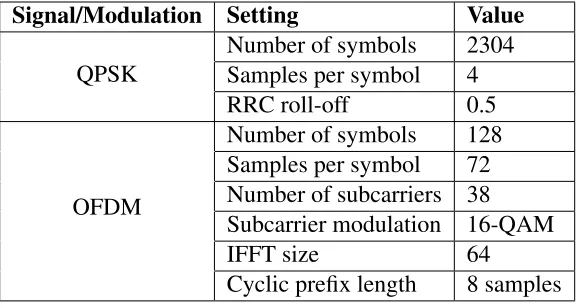
Two input signals are tested: a QPSK signal and an OFDM signal. Both in-put signals have a length of 9216 samples. Signal settings are summarized in Table 3.1. The QPSK signal is pulse shaped with a square root raised cosine with roll-off equal to 0.5. The OFDM signal contains 38 subcarriers, all of which are 16-QAM modulated at 64 samples per symbol with rectan-gular pulse shaping. A cyclic prefix of 8 samples is applied to each symbol to yield a total of 72 samples per symbol. AWGN is applied to both signals. Note that the signal length of 9216 samples means that 72 128-point FFTs will be computed for each algorithm.

Signal/Modulation Setting Value

QPSK

Number of symbols 2304 Samples per symbol 4

RRC roll-off 0.5

OFDM

Number of symbols 128 Samples per symbol 72 Number of subcarriers 38 Subcarrier modulation 16-QAM

IFFT size 64

Cyclic prefix length 8 samples

Table 3.1: Setup of QPSK and OFDM Test Signals

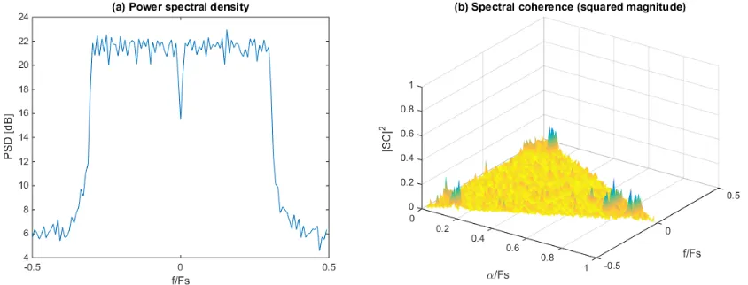
that the features in the spectral coherence of the OFDM signal are much weaker than the features in the QPSK signal. Also note that in the OFDM signal, spectral correlation of the individual 16-QAM modulated subcarriers does not appear. Even with a longer signal and larger FFT size, spectral correlation in individual subcarriers is not seen; the only apparent spectral correlation is related to the outside edges of the OFDM signal. The overlap between subcarriers appears to cancel out individual spectral correlation. We also observe that the cyclostationary features of the the QPSK signal are heavily diminished in low SNR.

Figure 3.1: PSD and spectral coherence of 9216-sample QPSK test signal at SNR = 15dB (Fs is the sampling frequency).

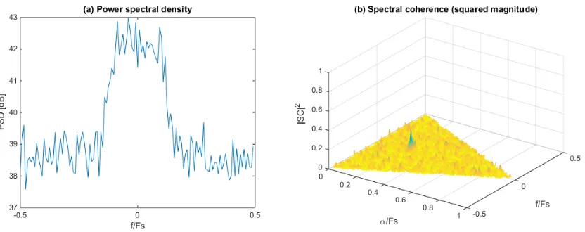
Figure 3.3: PSD and spectral coherence of 9216-sample QPSK test signal at SNR = -5dB (Fs is the sampling frequency).

3.3.2 Results

Figure 3.4 shows the resulting PD across SNR for both test signals, with

thresholds set so that PF A = 0.1. Figure 3.5 shows the resulting receiver

operating characteristic (ROC) curves with SNR held constant. The ED algorithm yields higher PD for a given PF A, for both QPSK and OFDM

signals, but especially for OFDM.

Figure 3.4: Probability of Detection vs SNR with fixed PF A=0.1 for (a) QPSK test signal

Figure 3.5: Detector ROC curves with fixed SNR for (a) QPSK test signal with SNR = -10 dB and (b) OFDM test signal with SNR = 5 dB.

Both algorithms see increases in performance when signal length is in-creased. In additional testing, we increased the signal length for the CD algorithm but kept the signal length the same for the ED algorithm. If sig-nal length is increased enough for the CD algorithm, eventually it meets the performance of the ED algorithm. Specifically, we saw that increasing the signal length 6.2 times (from 9216 samples to 57344 samples) caused the curve for the CD algorithm to match the curve of the ED algorithm in Figure 3.4(a). In other words, the CD algorithm required 6.2 times the sens-ing time to meet the performance of the ED algorithm for detection of the QPSK signal.

3.3.3 Conclusion

a range of frequencies to cover a very wide bandwidth. For wideband im-plementation the duration of a full scan may be too long to be useful for a cognitive radio. Additionally, wideband CD implementations would need to apply significant overlap between each band to sense. This is because a partially captured signal at the edge of the receiver bandwidth may not produce any features in the spectral coherence (mentioned in section 2.2.6). The only time the energy detection algorithm may fail is when the en-tire band of frequencies is occupied by signals, without guard bands. In that case the value for the noise floor estimate may be so inaccurate that the algorithm will not produce expected performance. However, the target plat-form’s 28 MHz maximum bandwidth is not expected to be entirely occupied by signals.

The simulations demonstrate the ineffectiveness of cyclostationary de-tection when using the maximum spectral coherence as a simple dede-tection statistic, especially for OFDM signals. For improved cyclostationary detec-tion in OFDM, the work in [16] suggests embedding unique cyclostadetec-tionary signatures in OFDM transmissions from cognitive radios. However this may not apply to detection of primary users, who can use any type of transmis-sion without embedded signatures.

3.4

Multiband Detection Algorithm

Based on simulation results for single-band detection, the energy detection algorithm was selected for further application. The single-band energy de-tection algorithm was modified to allow for dede-tection of signals across mul-tiple bands. The modified algorithm considers individual PSD bins instead of the maximum of all PSD bins. The modification also adds a metric to rank the strength of each spectrum hole. A higher hole ranking means the frequency bin is more likely to truly be a hole. The multiband algorithm is described as follows:

no windowing functions or overlap between FFTs.

X[k] = NF−1

X

n=0

x[n]·e−j2π

k

NFn _(3.10)

2. Compute the power spectral density (PSD) using the average squared magnitude of the FFTs.

Sxx[k] =

E[|X[k]|2_]

NF

(3.11)

3. Find the minimum PSD value and use it as an estimate of the noise floor.

4. Set the detection threshold T hED to be the minimum PSD value

mul-tiplied by fixed scaling factorSF.

T hED = min{Sxx[k]} ·SF (3.12)

5. For every frequency bin with PSD ≥ T hED, assert that a signal is

present in the band corresponding to that frequency bin.

Sxx[k] ≥T hED : signal present in frequency bink (3.13)

6. For each frequency bin that is a hole (meaning PSD < T hED), divide

T hED by the bin’s PSD value to produce the hole ranking metric.

Hole rank[k] = T hED

Sxx[k]

(3.14)

Note that PF A is now defined on a per-bin basis, meaning PF A is the

3.5

Simulation of Multiband Algorithm

The same QPSK and OFDM test signals used in the single-band simulation (shown in Figures 3.1 and 3.2) were used to test the multiband algorithm with AWGN. Also as in the single-band simulation, an FFT size of NF=128

was used. Two performance metrics were used to assess the multiband algo-rithm. The first metric is the average percentage of signal power detected in a signal’s bandwidth. The second metric is the probability to detect at least 90% of the power in a signal’s bandwidth (PD,90). We define the signal’s

bandwidth as the range of frequencies around the center frequency which contain 99.5% of the signal’s power. We test these performance metrics against different levels of in-band SNR; defined as the ratio of signal power to noise power inside the signal’s bandwidth.

3.5.1 Results

Figure 3.6a shows the average percent of signal power detected in the sig-nal’s bandwidth across in-band SNR. Figure 3.6b shows the resulting prob-ability of detecting 90% of the power in the signal’s bandwidth across in-band SNR. Thresholds corresponding to a PF A of 0.1 and 0.01 were used.

Slightly worse performance is seen from the OFDM signal at lower SNRs. This may be caused by the wider bandwidth of the OFDM signal (74% of the sampling bandwidth) vs the QPSK signal (35% of the sampling band-width). The wider bandwidth leaves fewer free bands for the algorithm’s noise floor estimate. Fewer free bands means that the estimate of the noise floor will be higher, resulting in a higher detection threshold. A higher de-tection threshold results in a lower probability of dede-tection.

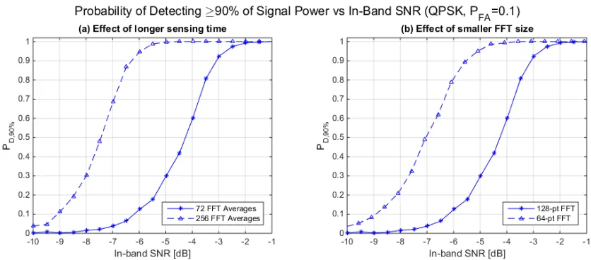
Figure 3.7 illustrates the effects of varying algorithm parameters (but keeping PF A the same) on detection performance for the QPSK test signal.

Figure 3.6: Performance of multiband energy detection algorithm. (a) Average percentage of signal power detected in signal’s bandwidth vs in-band SNR (b) Probability of detecting at least 90% of the power in signal’s bandwidth vs in-band SNR

naturally smooths each FFT and (2) more successive FFTs will be averaged. The trade-off is a decrease in the frequency resolution of the detector.

Figure 3.7: Effects on detection performance (a) increased sensing time (and therefore number of FFT averages) and (b) decreased FFT size.

3.5.2 Remarks for Implementation

Chapter 4

Implementation

4.1

SDR Platform

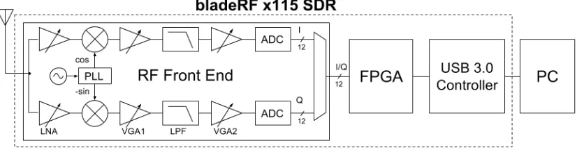
The implementation platform is the bladeRF x115 USB 3.0 software-defined radio, produced by Nuand LLC. The bladeRF can tune from 0.3 GHz to 3.8 GHz and can transmit/receive 28 MHz of instantaneous bandwidth with a 40 Msps sampling rate and 12-bit sampling resolution. The bladeRF con-tains an Altera Cyclone IV E FPGA with 115k logic elements which sits between a Lime Micro LMS6002D field-programmable RF transceiver and a Cypress FX3 USB 3.0 controller. The board interfaces with a host PC through its USB 3.0 port. The board’s FPGA allows signal processing to be performed in hardware in addition to software on the host PC. The de-fault FPGA bitstream contains an Altera Nios II soft processor for command and control (setting the frequency, gains, etc.) and a datapath to transfer IQ samples to/from the FX3 chip. The soft processor interfaces with the FX3 via UART and interfaces with the LMS6002D through SPI. The datapath interfaces with the FX3 via GPIF II and interfaces with the LMS6002D’s DACs/ADCs via a direct simple protocol. Figure 4.1 shows a block dia-gram of the implementation platform. The TX chain in the RF front end is unused in the implementation and was therefore omitted from the diagram.

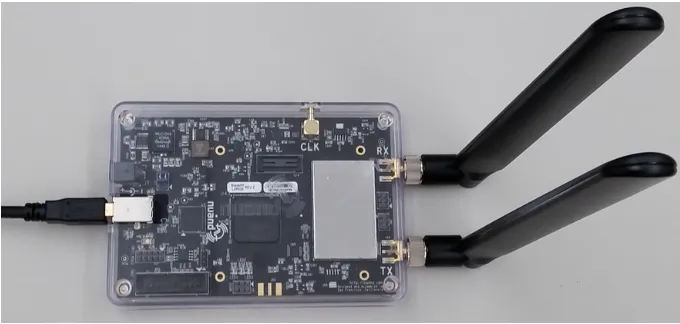
Figure 4.2 shows a photograph of the actual bladeRF device, with USB cable plugged in and antennas attached to the transmit and receive ports.

Figure 4.2: Image of bladeRF device

4.2

Implementation Overview

The detector implementation applies the proposed multiband energy detec-tion algorithm to cover a wide bandwidth for cognitive radio applicadetec-tions. Although the bladeRF can only receive 28 MHz of instantaneous bandwidth, the implementation scans GHz ranges by repeatedly changing the receive frequency and performing the multiband energy detection algorithm at each frequency. Figure 4.3 illustrates the the detector’s method of operation over a wide bandwidth.

The frequencies to scan are software-configurable; the maximum number of frequencies is 125 which can cover the bladeRF’s entire 0.3 GHz - 3.8 GHz range. The larger the frequency range, the more time each full scan requires. We refer to the full scan time as the latency. This latency represents the total sensing and processing time for each full scan. The latency of a full scan (tscan) is equal to the number of frequencies (Nf req) multiplied

by the sum of the sensing time per band (tsense,band) and the retune time

(tretune), shown in equation 4.1. Additional delay at the end of a full scan

calculation.

tscan = (tsense,band +tretune)·Nf req (4.1)

For covering the bladeRF’s entire 3.5 GHz range, the latency of each full scan is roughly 169 ms. Retune time is not instant, since it involves adjust-ing parameters of the RF front end’s phase-locked loop to guarantee lock via SPI transactions. The implementation’s retune time was determined to be 532.9 µs (see Section 5.3.1) and the sensing time per band is 819.2 µs. The sensing time per band refers to the amount of time spent receiving samples for an individual 28 MHz band, and is determined by the sampling rate and number of samples received per band. The implementation detects holes with a resolution of 314.6 kHz.

4.3

Implementation Architecture

The implementation performs all processing on the FPGA. Figure 4.4 shows a diagram of the detector architecture. The architecture consists of a soft-ware program (running on the Nios II soft processor) for frequency tuning and control, and a hardware datapath for signal processing and hole detec-tion. Receiver amplifier gains in the RF front end were set to constant values rather than different values based on frequency. No automatic gain control was used. Implementation specifications and settings are summarized in Table 4.1.

Figure 4.4: Implementation Architecture

Specification/Setting Value

IQ sampling rate 40 Msps Instantaneous bandwidth 28 MHz

FFT size 1281

Frequency resolution 314.6 kHz IQ samples per band 32768 Sensing time per band 819.2µs Number of FFT averages

per band 256

Table 4.1: Implementation Specifications and Settings

4.3.1 Hardware datapath

The hardware datapath refers to all blocks inside the FPGA in Figure 4.4 be-sides the Nios CPU and 16 KB RAM. For each frequency, the hardware dat-apath receives 32768 IQ samples at 40 Msps (for a sensing time of 819.2µs) and performs successive 128-point FFTs. Although the 40 Msps sampling rate produces a received bandwidth of 40 MHz (-20 MHz to +20 MHz), the lowpass filter in the RF front end reduces the passband bandwidth to 28 MHz (-14 MHz to +14 MHz). The FFT frequency bins outside of the 28 MHz lowpass filter bandwidth are discarded, reducing the number of fre-quency bins from 128 to 89. The signal is oversampled at 40 Msps to reduce aliasing. The squared magnitude of the FFT results are averaged to produce a PSD estimate. Each PSD estimate uses 256 FFT results for averaging. The minimum value of this PSD estimate is multiplied by a fixed scaling factor to produce the detection threshold. Frequency bins which contain PSD val-ues less than the threshold are deemed spectrum holes. Spectrum holes are ranked by the division of the threshold value by the individual PSD value.

4.3.2 Nios software

The Nios program cycles through a frequency table stored in attached em-bedded RAM and tunes the RF front end to each frequency via SPI. Once tuning to a certain frequency is complete, the program asserts a control register bit which tells the hardware datapath to receive samples. Once 32768 samples have been received the datapath interrupts the Nios CPU, after which the Nios program tunes to the next frequency and repeats.

4.3.3 PC interface

to the Nios program for storage in its RAM. To enable the detector the PC software sends a ’start’ packet to the Nios program, after which the detector begins continously scanning; repeating until the PC software sends a ’stop’ packet. The detector outputs one 32-bit sample for each frequency bin. The output sample consists of a single ’hole’ bit (1=hole, 0=signal), a 7-bit hole ranking, and a 24-bit PSD value for visualization purposes.

4.4

Details

4.4.1 Design

The FPGA logic was designed with VHDL. Two Altera Intellectual Property (IP) cores were used as part of the design: the 128-point FFT and a pipelined divider for calculating the hole ranking. The datapath processes samples in pipelined fashion, meaning that the outputs of one module are fed serially into the next module; with one sample per clock cycle. The serial transfer of samples allowed the datapath to be very efficient in hardware resources, since multiple parallel clones of the same hardware block were not needed. In order to sample at 40 Msps, the FPGA clock rate was set to 80 MHz (it must be double the sampling rate to acquire both the I and Q samples from the LMS6002D). Additionally, the Nios CPU ran at a clock rate of 80 MHz. Both the Nios software and the PC software for receiving detector output samples were written in C. A program for real-time visualization of PSD and holes was written in MATLAB.

4.4.2 DC Offset Handling

value was computed by receiving a large number of samples and recording the average I value and average Q value. The FPGA would subtract the DC offset from the received IQ signal on the fly. However, this proved to be ineffective, as the DC offset tended to quickly change over time causing the spike to still be seen at unacceptable levels. Methods of analog correction in the LMS6002D also proved to not be precise enough to completely remove the DC spike in the spectrum. Thus the DC PSD value was ignored and estimated using adjacent bins. Other implementations may require dynamic DC offset cancellation if the true PSD value of the DC bin is desired.

4.4.3 Fixed-point Bit Growth

Fixed-point arithmetic causes large bit growth; especially in multiplications. When results are rounded or truncated to reduce bit growth, precision loss occurs. In order to reduce this, the implementation performs minimal bit reduction in the FPGA. 12-bit I and Q input samples are passed to the FFT block which outputs 12-bit real and imaginary parts of the FFT along with a scaling exponent. After power calculation and application of the scaling exponent (not shown in Figure 4.4), the squared magnitude FFT samples are 39-bits long. The averaging block computes the sum of 256 39-bit samples, requiring 47 bits for each sum, then removes the 8 least significant bits to divide by 256 and output a 39-bit average (PSD). The minimum PSD value along with DC estimation are computed on the fly. The scale factor is stored in a 13-bit Q1.12 number. The threshold is computed by multiplication with the scaling factor followed by removal of the fractional bits.

4.4.4 Antenna and Frequency Considerations

detector. Therefore, the detector should not be applied to frequency bands where the antenna gain is not flat across the entire band. The implementa-tion can still work at frequency ranges in which the antenna has low gain, as long as the gain is flat across each 28 MHz band. However, the reduced SNR may significantly reduce the probability of detection. Dipole anten-nas with a frequency range of 698-2700 MHz were used for testing of the implementation with real-world signals.

4.5

Resource Utilization

The reported FPGA resource utilization accounts only for the hole detector hardware. This includes the datapath hardware, Nios system hardware re-lated to the hole detector (CPU, RAM, and interface peripherals), and hard-ware for interfacing with the RF front end. Other logic, including unused logic (i.e. the TX path) and logic used to transfer output samples to the PC through the FX3 chip, is not considered. Resource utilization is summarized in Table 4.2. The detector used an average of 8.8% of available resources on the Altera Cyclone IV E FPGA.

Resource Usage Percentage

Datapath Nios +

Interfaces Total of FPGA

4-input LUT 10680 1391 12071 10.5%

1-bit Register 9265 934 10199 8.9%

18x18 Multiplier 17 0 17 6.4%

8 Kb Memory Block 22 19 41 9.5%

Table 4.2: FPGA Resource Utilization of Hole Detector

4.6

Requirements for Implementation

programmable RF front end that can quickly change its local oscillator fre-quency over a wide range. Without dynamic retuning, the wide range of frequencies needed by cognitive radios cannot be sensed. As mentioned in section 3.1, the implemented energy detection algorithm only performs well if the received bandwidth at each frequency is not completely occupied by signals. Therefore a fairly wide instantaneous bandwidth is needed for the implementation. Given that typical real-world transmissions are 20 MHz or less in bandwidth, we recommend an instantaneous bandwidth greater than 25 MHz for low probability that the entire band is occupied by signals. If wider bandwidth signals are expected, a higher instantaneous bandwidth is required for good performance from the algorithm.

4.7

Source Code

Implementation source code, including both VHDL hardware description and C software, has been provided online at:

Chapter 5

Experiments and Results

After finalizing the detector implementation, experiments were performed on the detector to assess its performance and uncover any implementation is-sues. Performance experiments were performed using wired channels. This chapter discusses implementation issues, experimental setup, and experi-mental outcomes.

5.1

Implementation Issues

Testing revealed some issues related to the analog nature of the RF front end.

5.1.1 Spurious Tones in Noise Spectrum

5.1.2 Analog Filter Frequency Response

Testing of the detector also revealed an issue with the lowpass filter inside the RF front end. The frequency response of the lowpass filter is not flat in-side the passband. The magnitude of the frequency response is lower around DC and higher around the cutoff frequency. Specifically, the magnitude is around 1 dB higher at the cutoff frequency than at DC. This issue was also noted in the work in [17]. This issue caused extra false alarms to be seen seen around the lower and upper ends of each 28 MHz frequency band (at baseband, the lower end corresponds to -14 MHz, and the upper end cor-responds to +14 MHz). When running the detector with a scaling factor produced by MATLAB simulations for PF A=0.1, an actual PF A of 0.4 was

seen. The detector’s scaling factor had to be increased to reach PF A=0.1.

The end result is that a higher detection probability is seen for frequencies near the cutoff frequency, and a lower detection probability is seen for fre-quencies around DC.

We identified a solution to this issue but did not have time to add the solution to the implementation. Although the shape of the filter response is not flat in the passband, it is consistent. Compensating for the shape of the filter response in the implementation would remove its unwanted ef-fects. Compensation must be applied to the PSD values directly before the minimum PSD is calculated and before any hole detection. Compensation values can be applied as a set of precomputed scaling factors stored in a read-only memory. The appropriate scaling factor would be selected based on the frequency index of the PSD value to scale.

5.2

Side Experiment: Noise Characterization

5.2.1 Noise Floor Variation

the receive antenna unattached and replaced with a 50-ohm terminator, in-ternal noise power from the RF front end varied by 20 dB between the lowest frequency (0.3 GHz) and the highest frequency (3.8 GHz). Simply attach-ing the antenna increased the observed noise power by 10-15 dB at certain frequency bands. Adjusting the orientation of the antenna also changed the observed noise power by 10-15 dB at certain frequencies. This confirms that a static estimate of the noise floor is not possible for energy detection. A dy-namic estimation technique, like the one used in the proposed algorithm, is needed for energy detection on realistic systems.

5.2.2 PSD and Spectral Coherence of Noise

We examined the PSD and spectral coherence of noise generated from the RF front end in order to compare it to simulated white Gaussian noise. The bladeRF with stock FPGA was used to receive 32768 samples at 40 Msps, with the low pass filter of the RF front end set to 28 MHz and a 50-ohm ter-minator attached to the receive port. The frequency was set to 1254 MHz. MATLAB software was used to compute successive 128-point FFTs of the received signal. As in the detector implementation, FFT bins outside of the 28 MHz filter bandwidth were discarded. We computed the PSD and spec-tral coherence using the same techniques as in the simulations in Chapter 3. As in implementation, the PSD of the DC bin was estimated using the mean PSD of the adjacent bins. Figure 5.1 shows the resulting PSD and spectral coherence estimates of the noise.

The non-flat shape of the PSD from the lowpass filter issue discussed in Section 5.1.2 is clearly seen. One spurious tone (issue discussed in Section 5.1.1) is also seen in the PSD plot at a frequency of 1267 MHz. The spec-tral coherence of the noise is mostly flat with a mean magnitude of around 0.1. Unexpectedly, the spurious tone produces a small peak in the spectral coherence magnitude equal 0.37 to at (f, α) = (1267 MHz, 0.63 MHz). The spurious tone produces more spectral correlation than the surrounding white noise. This means that spurious tones could also cause false alarm issues in cyclostationary detection algorithms.

5.3

Setup of Performance Experiments

Figure 5.2 illustrates the experimental setup. The setup consisted of three bladeRF SDR devices transmitting through SMA cables to one receiver bladeRF performing hole detection. The three transmitted signals were added using a 4:1 RF combiner. After the combiner, two 30 dB attenuators were applied to protect the receiving device and reduce SNR. All bladeRF devices were connected through USB 3.0 to a PC.

Figure 5.2: Experimental Setup

Msps was used, resulting in a signal bandwidth of 5 MHz. The bandwidth of the lowpass filter in the transmit chain of the RF front end was set to 12 MHz. The number of symbols in the OFDM signal was increased to 896 for a signal length of 64512 samples. For transmission of the OFDM sig-nal, a sampling rate of 24 Msps was used, resulting in a signal bandwidth of 16.5 MHz. The bandwidth of the lowpass filter in the transmit chain of the RF front end was set to 20 MHz. Each signal transmission was repeated indefinitely to result in a continuous transmission.

5.3.1 Detector Parameters and Characteristics

The detector parameters used for performance experiments as well as la-tency characteristics are summarized in Table 5.1. The detector’s frequency table was configured to scan frequencies from 1308 MHz to 2288 MHz for a total sensing bandwidth of 980 MHz. This configuration involves 35 fre-quency retune operations for each full scan of the detector. The scaling fac-tor for the detecfac-tor implementation was set to 1.455, producing a measured

PF A of 0.09. PF A was measured by running the detector with a 50-ohm

ter-minator on its receive port, and counting the number of false alarms across all frequencies; repeating for 500 iterations. As noted in Section 5.1.2, im-perfections in the lowpass filter inside the RF front end caused the scaling factor for implementation to differ from the expected scaling factor from simulation.

Parameter/Characteristic Value

Scaling factor 1.455

PF A 0.09

Number of frequencies 35

Frequency range 1308 - 2288 MHz

Total bandwidth 980 MHz

Retune time 532.9µs

Full scan time 47.3 ms

Table 5.1: Detector Parameters and Characteristics

scan was 47.3 ms. Dividing the total latency by the number of frequencies (35) and subtracting the chosen sensing time per band (819.2 µs) yields an average retune time of 532.9 µs.

5.4

Results

5.4.1 Single Transmission

This experiment was performed with a signle transmission from one bladeRF device. To eliminate bias from the analog filter issue discussed in Section 5.1.2, two different carrier frequencies were used. One carrier frequency was placed at the center of one of the detector’s frequency bands, and the other carrier frequency was placed at the edge of one of the detector’s fre-quency bands. The carrier frequencies used were 2134 MHz and 2148 MHz. The performance metric tested was the probability of detecting at least 90% of the power in the signal’s bandwidth (PD,90). As mentioned in

Sec-tion 3.5 (simulaSec-tion of multiband algorithm), we define the signal’s band-width as the range of frequencies around the center frequency which contain 99.5% of the signal’s power. For each test signal (QPSK and OFDM), the detection probability results from the two carrier frequencies used were av-eraged to produced a final number for PD,90.

Figure 5.3 shows the resultingPD,90 of the detector across in-band SNR

for both the QPSK signal and the OFDM. We see that for a given in-band SNR, PD,90 is higher for the QPSK signal than for the OFDM signal. As

PF A value.

Figure 5.3: Detector performance for a single continuous transmission and fixed PF A =

0.09

5.4.2 Multiple Transmissions

This experiment was performed with three continuous transmissions from three bladeRF devices. The three frequencies used were 1443.4 MHz, 1648.6 MHz, and 2111.7 MHz. Tests for QPSK signals and OFDM signals were kept separate. The transmit gain of each transmission was adjusted so that all transmissions had the same in-band SNR (+/- 0.5 dB). The gains were then increased or decreased together in order to vary in-band SNR.

The performance metric tested was the probability of detecting at least 90% of the power in every signal (P_D,all₉₀). Essentially, this is the probability to detect all signals at any given time. Figure 5.5 shows the resulting P_D,all₉₀

across in-band SNR, for both QPSK transmissions and OFDM transmis-sions. Interestingly, the performance of the detector with the OFDM signals is about the same as the performance with the QPSK signals.

Figure 5.5: Detector performance for three continuous transmissions

5.4.3 Example Detector Output

The frequency range of the output plots has been restricted to a small 112 MHz window. The vertical dotted lines show the boundaries between each 28 MHz band of the detector. In the hole detection plot (Figure 5.6(b)) the shaded areas are detected holes. Note the presence of unwanted spikes in the power spectral density due to the tones discussed in Section 5.1.1. Also note that the false alarms seen in the holes plot are expected because the de-tector was designed for a PF A of 0.09. The detector successfully identifies

spectrum holes and classifies the three signals as non-holes.

Chapter 6

Conclusion

This research consisted of the design, simulation, implementation, and anal-ysis of a spectrum holes detector for cognitive radio applications. Single-band cyclostationary detection and energy detection algorithms which do not require a-priori knowledge of noise power were compared and ana-lyzed. Simulations concluded that the performance of the energy detection algorithm was significantly higher than than the performance of the cyclo-stationary algorithm. The energy detection algorithm produced a higher

PD for a given PF A and fixed sensing time. A multiband energy detection

algorithm suitable for wideband implementation was proposed. The open-source SDR implementation demonstrated efficient application of the algo-rithm for an extremely wide bandwidth, with reasonable latency, suitable for usage in cognitive radios. Implementation issues and hardware/resource requirements were described in detail.

Bibliography

[1] Molisch, Andreas F,Wireless Communications, Second Edition. John Wiley and Sons, Ltd, 2011, page 506.

[2] I. S. Association, “Cognitive Wireless RAN Medium Access Control

and Physical Layer Specifications: Policies and Procedures for

Opera-tion in TV bands,”IEEE Standard 802.22-2011, p. 447, Jun. 2011. [3] S. Haykin, “Cognitive radio: brain-empowered wireless

communica-tions,” IEEE Journal on Selected Areas in Communications, vol. 23, no. 2, pp. 201–220, Feb 2005.

[4] Federal Communications Commission. White Space Database

Administration. Accessed 2017-04-19. [Online]. Available:

https://www.fcc.gov/general/white-space-database-administration

[5] D. Cabric, S. M. Mishra, and R. W. Brodersen, “Implementation issues

in spectrum sensing for cognitive radios,” in Conference Record of the Thirty-Eighth Asilomar Conference on Signals, Systems and Comput-ers, 2004., vol. 1, Nov 2004, pp. 772–776 Vol.1.

[6] T. Yucek and H. Arslan, “A survey of spectrum sensing algorithms for

cognitive radio applications,” IEEE Communications Surveys Tutori-als, vol. 11, no. 1, pp. 116–130, First 2009.

[7] M. L´opez-Ben´ıtez and F. Casadevall, “Improved energy detection

spectrum sensing for cognitive radio,” IET communications, vol. 6, no. 8, pp. 785–796, 2012.

[8] S. Atapattu, C. Tellambura, and H. Jiang, “Energy Detection Based

Transactions on Wireless Communications, vol. 10, no. 4, pp. 1232– 1241, April 2011.

[9] A. Mariani, A. Giorgetti, and M. Chiani, “Effects of Noise Power

Esti-mation on Energy Detection for Cognitive Radio Applications,” IEEE Transactions on Communications, vol. 59, no. 12, pp. 3410–3420, De-cember 2011.

[10] B. Shent, L. Huang, C. Zhao, Z. Zhou, and K. Kwak, “Energy

De-tection Based Spectrum Sensing for Cognitive Radios in Noise of

Un-certain Power,” in 2008 International Symposium on Communications and Information Technologies, Oct 2008, pp. 628–633.

[11] S. Enserink and D. Cochran, “A cyclostationary feature detector,” in

Proceedings of 1994 28th Asilomar Conference on Signals, Systems and Computers, vol. 2, Oct 1994, pp. 806–810 vol.2.

[12] K. Kim, I. A. Akbar, K. K. Bae, J. S. Um, C. M. Spooner, and J. H.

Reed, “Cyclostationary Approaches to Signal Detection and

Classifi-cation in Cognitive Radio,” in 2007 2nd IEEE International Sympo-sium on New Frontiers in Dynamic Spectrum Access Networks, April 2007, pp. 212–215.

[13] A. Tkachenko, D. Cabric, and R. W. Brodersen, “Cyclostationary

Fea-ture Detector Experiments Using Reconfigurable BEE2,” in 2007 2nd IEEE International Symposium on New Frontiers in Dynamic Spec-trum Access Networks, April 2007, pp. 216–219.

[14] S. Maleki, A. Pandharipande, and G. Leus, “Two-stage spectrum

[15] W. Yue and B. Zheng, “A two-stage spectrum sensing technique in

cognitive radio systems based on combining energy detection and

one-order cyclostationary feature detection,” inProceedings of the 2009 In-ternational Symposium on Web Information Systems and Applications (WISA09), 2009, pp. 327–330.

[16] P. D. Sutton, K. E. Nolan, and L. E. Doyle, “Cyclostationary

Sig-natures for Rendezvous in OFDM-Based Dynamic Spectrum Access

Networks,” in2007 2nd IEEE International Symposium on New Fron-tiers in Dynamic Spectrum Access Networks, April 2007, pp. 220–231. [17] S. M. Mishra, S. ten Brink, R. Mahadevappa, and R. W. Brodersen,

“Cognitive Technology for Ultra-Wideband/WiMax Coexistence,” in