The Factor Structure of Visual Imagery and Spatial Abilities
Lorelle J. Burton and Gerard J. Fogarty
The University of Southern Queensland
Mailing Address: Dr Lorelle J. Burton
Department of Psychology
The University of Southern Queensland
Toowoomba Queensland 4350
Australia
Abstract
The Factor Structure of Visual Imagery and Spatial Abilities
In the factor-analytic literature, there is limited information on the relationship between clearly defined cognitive ability factors and measures of visual imagery. Carroll (1993) recently proposed that an independent Imagery (IM) factor might be discriminable from other first-order spatial factors. He defined the hypothetical Imagery factor as “the ability in forming internal mental representations of visual patterns, and in using such representation in solving spatial problems” (Carroll, p. 363). Carroll advocated that research was required to clarify the theoretical status of the hypothetical Imagery factor, and also recommended research into the distinction between this proposed Imagery factor and the Visualisation sub-factor of spatial ability. The main aim of the current study was to investigate whether visual imagery can be regarded as a separable component of psychometric spatial ability.
To investigate the status of imagery ability within the structure of intelligence, it is necessary to consider firstly the classification of the major spatial abilities within the domain of visual perception. In perhaps the most comprehensive review of the psychometric literature available to date, Carroll (1993) supported the independent existence of a number of factors in the spatial ability domain. He provided empirical evidence for five major discriminable first-order spatial factors: Visualisation (VZ), Speeded Rotation (SR), Closure Speed (CS), Flexibility of Closure (CF), and Perceptual Speed (P). The Visual Memory (MV) factor was also shown to share substantial correlation with the broad General Visualisation (Gv) factor. The Imagery (IM) factor was recognised by Carroll as one other potential narrow factor of spatial ability worthy of specific investigation.
The prolonged debate over the status of the visual imagery construct is in part due to the lack of a unique operational definition. Visual imagery may be
conceptualised as either an undifferentiated, single ability or as a multidimensional construct. Kosslyn (1980) argued that visual imagery may be decomposed into several subprocesses, including generation, maintenance, and transformation processes. Denis (1991) stressed the importance of identifying those processes used to generate images and also those processes that are needed to maintain the image once it has been formed. Along these lines, it is common to see researchers defining visual imagery in terms of the subjective qualities of vividness and control (Poltrock & Agnoli, 1986). Vividness refers to the liveliness, clarity, sharpness, and
distinctiveness of the image (Marks, 1995; McKelvie, 1995a, McKelvie, 1995b). A controlled image is under the volitional control of the individual; it can be maintained and transformed at will (Marks, 1973). Recent factorial evidence that will be
reviewed later supports the notion that visual imagery is a multidimensional construct, covering such aspects as the clarity, controllability, maintenance, and vividness of mental representations that have percept-like qualities (Dean, 1994).
Secondly, self-report questionnaires of imagery vividness and control remain the oldest, yet most popular, technique for assessing individual differences in imagery ability. These traditional self-report imagery questionnaires tend to conceptualise imagery as a unidimensional construct (Dean, 1994). Self-report measures of imagery vividness include the shortened version of Betts' (1909) Questionnaire Upon Mental Imagery (QMI, Sheehan, 1967), and Marks' (1973) Vividness of Visual Imagery Questionnaire (VVIQ). Gordon's (1949) Test of Visual Imagery Control (TVIC), on the other hand, is commonly employed as a measure of one's ability to control and manipulate visual images. In these questionnaires, participants are required to visualise familiar scenes and to rate the vividness or ease of control of their images according to a likert-type rating scale. A large body of empirical evidence supports the internal consistency of these instruments (see Richardson, 1994 for a review). Furthermore, self-report imagery ratings of vividness (VVIQ) and control (TVIC) tend to correlate moderately well with each other (Richardson, 1983) and to load on a common factor (Lorenz & Neisser, 1985). However, further research is required to establish the relationship between these subjective measures of imaginal experience and conventional spatial tests presumed to require imagery in their performance.
Factorial studies of imagery ability suggest that the subjective qualities of imagery as measured by self-report techniques are unrelated to spatial test performance (e.g., Dean, 1994; Di Vesta, Ingersoll, & Sunshine, 1971; Kosslyn, Brunn, Cave, & Wallach, 1984; Poltrock & Agnoli, 1986; Poltrock & Brown, 1984; Richardson, 1977, 1983). For example, Kosslyn et al. (1984) took an information-processing approach to the study of individual differences in imagery ability. They compiled a battery of experimental tasks to reflect the multiple dimensions of imagery processing posited in the Kosslyn and Schwartz (1977, 1978) theory of image representation. The broad range of correlations among performance measures for the different experimental tasks (mean r = .28) indicated that visual imagery can be differentiated into distinct processing modules, such as image generation, image inspection, and various image transformation and rotation abilities. Cluster and factor analyses of the correlation matrix indicated that spatial task performance was
dependent upon the maintenance of a high quality image (accuracy) and efficient image inspection and transformation processes (speed). Self-report imagery vividness (VVIQ) did not correlate with any performance measure, apart from the resolution process. This finding implied that self-report imagery vividness was related to characteristics of the visual buffer, but distinct from those aspects of imagery ability measured by the experimental imagery tasks.
A related study by Poltrock and Brown (1984) investigated the relationship between individual differences in visual imagery and spatial visualisation. They developed six experimental tasks to tap the processes and structures outlined in Kosslyn’s (1980) theory of mental imagery. The design included measures of image quality (accuracy) and the efficiency of the processes of image generation, image rotation, image scanning, adding and subtracting detail in images, and image
integration. The correlations among the experimental imagery measures were shown to be relatively low (mean r = .10) and nonsignificant (p > .05). This finding
suggested that imagery ability consisted of a number of independent cognitive processes. Furthermore, significant intercorrelation was evident between the
transformation and inspection processes were necessary for successful spatial task performance. In contrast, self-report imagery measures were not related to spatial test performance (p > .05). This finding supported the notion that the self-report imagery questionnaires tap a unique aspect of visual imagery ability.
Poltrock and Agnoli (1986) further examined the relationship between visual imagery and spatial abilities. Their research similarly supported the treatment of visual imagery as a multidimensional construct. In addition, they concluded that visual imagery was used to solve spatial problems but that the self-report
questionnaires (e.g., VVIQ and TVIC) measured qualities of imagery that played no central role in the performance of spatial tests. In short, the two measurement
techniques tap different aspects of imagery - - the subjective aspects of imagery (e.g., vividness and control) measured by self-report questionnaires are functionally distinct from those aspects of imagery measured by conventional tests of spatial ability.
Aims of the Present Study
The current study was designed to investigate the nature of Carroll’s (1993) hypothetical Imagery (IM) construct. The study builds upon these earlier findings, bringing together a wide range of self-report and experimental imagery tasks in a battery that also contains markers for well-replicated primary spatial factors. The main aim was to establish whether a primary IM factor can be identified as a separate dimension of individual differences in the spatial ability domain. Of particular
relevance to this question was the issue of examining the relationship between visual imagery and other well-replicated spatial primary abilities. A central proposition of the present research was that the ability to form and manipulate abstract, visual images will emerge as a separate, narrow ability factor of spatial intelligence (Gv). Accordingly, both exploratory and confirmatory factor analytic techniques were used to establish the sources of variance in individual differences in visual imagery ability. For a detailed exposition of the rationale underlying such an approach see Carroll (1995).
Since the current study was designed within the framework of fluid (Gf) and crystallized (Gc) intelligence (henceforth referred to as Gf-Gc theory), the test battery included a representative sample of markers capable of yielding adequate measures of the broad ability clusters of Gf, Gc, and Gv. The study was designed to move beyond analysis of VZ and SR tasks to include a wider representation of spatial primaries. To this end, the relationship of the hypothetical IM factor with each of the major spatial factors (i.e., VZ, SR, CF, P, CS, and MV) was examined.
The test battery also comprised the popular self-report questionnaires of imagery vividness and control. In addition, the battery included experimental measures of imagery ability derived from the research of Kosslyn et al. (1984), Poltrock and Brown (1984), and Juhel (1991). In these experimental tasks, separate speed and accuracy measures were examined to determine the speed-level
components of imagery ability. Accuracy measures were taken to reflect aspects of image quality (e.g., the ability to generate and maintain a clear, vivid mental image), while speed of processing measures were taken to reflect efficiency of image
spatial-imagery tasks and help to provide a clearer understanding of the status of the posited IM factor.
Finally, the current study was designed to introduce the two new imagery measures that capitalise on some developments in the measurement area. Both the Dean and Morris (1991, 1995) imagery questionnaire and the Finke, Pinker, and Farah (1989) creative imagery tasks were examined from a differential perspective. Firstly, the new-format imagery questionnaire by Dean and Morris was included to tap various aspects of image quality, including generation, maintenance, control, vividness, and rotation processes. In this questionnaire, participants are required to imagine a static and/or rotated spatial shape. This procedure stands in contrast to other imagery vividness questionnaires where participants are required to introspect on the image of everyday items recalled from long-term memory. Secondly, two sets of the creative imagery tasks developed by Finke et al. (1989) were adapted for inclusion in the test battery. These tasks required participants to listen to a verbal description and to provide a written interpretation of the imagery content. The Emergent Forms task was included as a measure of participants’ ability to mentally detect emergent patterns in a synthesised image. The Transformation task measured participants’ ability to identify a final pattern after transforming a mental image in specified ways.
The second aim of the study was to test the proposition that self-report measures of visual imagery ability are unrelated to measures of spatial ability. The lack of relationship has already been demonstrated in earlier studies using
questionnaires that tap the subjective imaginal experience of familiar scenes (see Kosslyn et al., 1984; Poltrock & Brown, 1984; Richardson, 1983). In the present study, self-report questionnaires that make use of objective, spatial stimuli were included along with purely subjective measures. It was hypothesised that the more stimulus-based self-report measures of visual imagery ability would correlate with spatial measures.
Method
Participants
A total of 213 participants (114 females) was involved in this study.
Approximately half of these were recruited from the adult population of the regional city of Toowoomba and its surrounding region. The remainder were undergraduate psychology students from the University of Southern Queensland (USQ) who participated to gain credit in their course. Overall, the sample exhibited variability with respect to age and education, although the majority of participants had academic qualifications equivalent to, or higher than, the junior certificate level (i.e., 10 years schooling). The average age of the participant pool was 26.32 years with a standard deviation of 8.91 years. The mean age of the females was 24.58 years, with an age range from 17 to 54 years. The males had a mean age of 28.33 years, with an age range from 17 to 59 years.
Materials
Reference tests.
Eight marker tests were included for the broad Gf and Gc abilities.
correct was scored as the dependent variable for each reference test (i.e., measures of level ability).
The four tests used to mark for the broad Gf factor involve basic manipulations of abstractions, rules, and logical relationships:
1. Letter Series(Gf1; Thurstone & Thurstone, 1965). 2. Number Series(Gf2; Thurstone & Thurstone, 1965). 3. Matrices(Gf3; Cattell & Cattell, 1965).
4. Word Grouping(Gf4; Thurstone & Thurstone, 1965).
Gc is often measured by tests requiring the demonstration of learning, such as vocabulary, or by primaries like verbal reasoning. The Ekstrom, French, Harman, and Dermen (1976) kit of factor-referenced cognitive tests was the source for the
following four tests used to mark for Gc ability: 5. Scrambled Words (Gc1).
6. Hidden Words (Gc2). 7. Incomplete Words (Gc3). 8. Vocabulary(Gc4).
The P factor was defined in the 1976 ETS factor kit as “speed in comparing figures or symbols, scanning to find figures or symbols, or carrying out other very simple tasks involving visual perception” (Ekstrom et al., 1976, p. 123). The Ekstrom et al. kit of factor-referenced cognitive tests was the source for the following three tests used to demarcate P ability:
9. Finding A’s (P1).
10. Number Comparison (P2). 11. Identical Pictures (P3).
The SR factor reflects the ability to perceive an object from different positions, and is usually defined by simple speeded tests involving rotations and/or reflections (Lohman, 1988). The following tests were included as markers for the SR factor:
12. Card Rotations(SR1; Ekstrom et al., 1976). 13. Cube Comparisons(SR2; Ekstrom et al., 1976).
14. Spatial Relations(SR3; Thurstone & Thurstone, 1965).
A characteristic of tests of the VZ factor is the requirement that the participant apprehend a spatial form, and rotate it in two or three dimensions before matching it with another spatial form (Eliot & Smith, 1983). Visualisation tests are often given under relatively unspeeded conditions to ascertain mastery level, compared with SR tests where scores are more dependent upon speed of performance (Carroll, 1993). The Ekstrom et al. (1976) kit of factor-referenced cognitive tests was the source for the following tests used to demarcate VZ ability:
15. Paper Form Board (VZ1). 16. Paper Folding (VZ2).
17. Surface Development (VZ3).
Tests of the CF factor reflect the ability to “break one gestalt and form another” (Lohman, Pellegrino, Alderton, & Regian, 1987, p. 265). Carroll (1993) noted that this CF factor is sometimes indistinguishable from the VZ factor of spatial ability, and may also share some variance with SR. The tests used to mark for CF ability were those included as markers in the 1976 ETS kit:
18. Hidden Patterns (CF2). 19. Copying (CF3).
the manual for the full set of 16 items. This test was later dropped from analyses because of poor reliability.
The CS factor reflects the “ability to identify quickly an incomplete or distorted picture” (Lohman et al., 1987, p. 266). The CS factor can be distinguished from the CF factor by the fact that tests of CS do not show any obvious closure to start with, and participants do not know what to look for, whereas in tests of CF, participants are required to detect a required configuration from a more complex pattern (Carroll, 1993). The 1976 ETS kit was the source for the following three tests used to mark for CS ability:
20. Gestalt Completion (CS1). 21. Concealed Words (CS2). 22. Snowy Pictures (CS3).
Ekstrom et al. (1976) defined the MV factor as “the ability to remember the configuration, location, and orientation of figural material” (p. 109). Although the status of the factor remains unclear in the psychometric literature, there is evidence for a visual memory factor “controlling performance on tasks in which the participant must form and retain a mental image or representation of a visual configuration that is not readily encodable in some other modality” (Carroll, 1993, p. 284). The 1976 ETS kit was the source for the following three tests used to mark for the MV factor:
23. Shape Memory (MV1). 24. Building Memory (MV2). 25. Map Memory (MV3).
Due to time constraints, for the Shape Memory and Building Memory tests, participants were allowed 3 minutes for memorising, and a further 3 minutes to complete the items, rather than the recommended 4 minutes for each section.
Creative imagery task measures.
Two sets of creative imagery tasks were developed on the basis of findings obtained by Finke et al. (1989). The first creative imagery task was constructed to ascertain individual differences in participants’ ability to “mentally inspect” their superimposed image for possible emergent forms. This task will henceforth be referred to as the Emergent Forms task. The second creative imagery task was a mental Transformation task that required participants to identify the final pattern after mentally transforming their image. All instructional material was based on the work of Finke et al., and was verbally presented to participants through lightweight headphones. A 3 s pause was provided between each step to allow participants enough time to form the image required. However, participants had control over the rate of presentation, and could press the pause button if they required more time to complete each step in the image sequence. In addition, participants were provided with a paper copy of the initial task instructions. A brief description of each task follows.
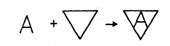
forms detected might include one small triangle, two larger triangles, a diamond shape, the letter “w”, and so on. Upon drawing the final pattern imagined, participants were requested to report any additional emergent forms that they could now detect, but that they had not previously seen in their image. The dependent variable was the total number of emergent forms (both symbolic and geometric forms) detected from imagery.
Figure 1. An example item from the Emergent Forms task. Participants were required to superimpose the letter A with an upside down triangle.
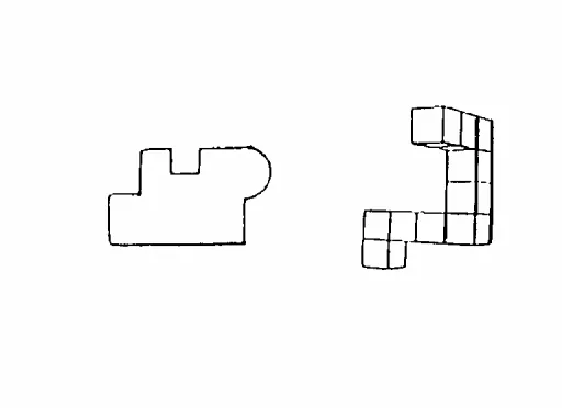
27. Transformation Task (Transform). In this 12-item task, participants were instructed to begin with a starting pattern, then to imagine transforming the pattern in specified ways and to report what the resulting pattern looked like. For example, as shown in Figure 2: "Imagine the letter B. (Pause) Rotate it 90 degrees to the left. (Pause) Put a triangle directly below it having the same width and pointing down. (Pause) Remove the horizontal line." (Finke et al., 1989, p. 62). In this case, a correct identification would be either a love heart or a double scoop ice-cream cone. For each item, participants were instructed to indicate whether they were able to correctly guess the identity of the final pattern at any stage prior to the final transformation step. At the end of each set of instructions, participants were required to write down the description of the identified final pattern on the response sheet provided. Finally, participants were asked to draw the final pattern imagined and to try to identify it from their drawing if they had not done so during imagery. Participants were also required to report any difficulties they may have had when transforming their image. A measure of participants' transformation ability was computed by totaling the number of correct pattern identifications made from imagery.
Figure 2. An example item from the Transformation task. Participants were required to generate and manipulate an image of the letter B and a triangle.
Self-report measures.
[image:9.595.131.463.559.617.2]mental rotation. The second shape was three-dimensional, and selected from the Vandenberg and Kuse (1978) test of mental rotation.
Figure 3. A two-dimensional CAB-S shape and a three-dimensional Vandenberg shape included on the imagery questionnaire developed by Dean and Morris (1995).
For both the CAB-S and Vandenberg shapes, participants were asked to rate each of the following 13 properties separately, and independently of the other shape. They were first asked to rate the image of the static shape on eight parameters: (a) ease of evocation, (b) detail, (c) clarity, (d) ease of maintenance, (e) detail change, (f) clarity change, (g) proportion, and (h) vividness. Participants were then required to imagine the shape rotating and to rate the image according to the following five properties: (a) ease of rotation, (b) detail during rotation, (c) clarity during rotation, (d) proportion during rotation, and (e) vividness during rotation. All item ratings were made on a scale of 1 (very poor) to 9 (very good). Additionally, participants were required to mark on the different shapes what parts they had imagined when the image was static and, similarly, mark the parts of the shape imagined during rotation. Total scale scores for each participant were computed for the following spatial shapes:
28. The CAB-S Questionnaire (CABSqnre). 29. Vandenberg Questionnaire (Vandqnre).
Secondly, participants completed the following questionnaires of imagery vividness and control:
30. Questionnaire Upon Mental Imagery (QMI). The QMI consists of 35 items designed to assess imagery vividness in seven sensory modalities - - visual, auditory, tactile, kinesthetic, gustatory, olfactory, and organic (Sheehan, 1967). For each sensory modality, participants were required to imagine five particular scenes, and to rate the vividness and clarity of each image by reference to a rating scale ranging from 1 (perfectly clear and as vivid as the actual experience) to 7 (no image present at all, you only “know” that you are thinking of the object).
31. Test of Visual Imagery Control (TVIC). The TVIC is a 12-item
to indicate their degree of imagery control according to the 3-point scale (yes, no, and unsure).
32. Vividness of Visual Imagery Questionnaire (VVIQ). The VVIQ was included as a supplementary measure of the vividness of visual imagery (Marks, 1973). Participants were required to rate the vividness of their imagery for familiar scenes by reference to a 5-point scale (1 = perfectly clear and as vivid as normal vision; 5 = no image at all, you only “know” that you are thinking of an object). Each of the 16 items in the scale was rated twice, once with the eyes open and once with them closed.
Experimental measures.
The seven experimental tasks used in this study were based on recent theories and research findings on the structure of the imagery system (e.g., Juhel, 1991; Kosslyn et al., 1984; Poltrock & Brown, 1984). Accuracy measures were taken to investigate the extent to which limitations in image quality might represent an important source of individual differences in imagery ability. Speed of processing measures were used to examine the efficiency of imagery processes, including those involved in image generation, image inspection, and image transformation. Other aspects of image process efficiency measured by these tasks included: efficiency of adding and subtracting detail to and from images, image maintenance, clarity and vividness of image processes, and visual memory abilities. It was anticipated that accuracy would be independent of the time required by those processes operating on the image data structures (see Carroll, 1993; Kyllonen, 1985; Roberts, 1995). A brief description of each task follows.
33. Picture Task (PictureRT). The Picture task was developed from the research of Poltrock and Brown (1984) to measure the efficiency of processes involved in generating images. In this task, participants were required to listen to the verbal description (presented through headphones as synthesised speech) of 20 familiar scenes and to press the space bar when a clear “mental picture or visual image” was formed. The time to form each image was measured (in deci seconds) from stimulus onset to the participant’s response.
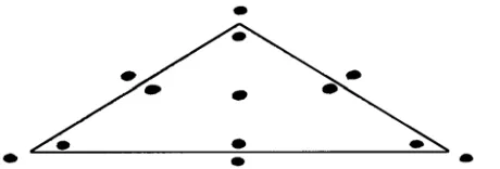
Figure 4. The 13 dot positions used in the Add and Subtract experimental imagery tasks.
35. Subtract Task (SubtractNC). The Subtract task was similar in design and procedure to the Add task, but with the aim of measuring the ability to mentally delete parts of an image (Poltrock & Brown, 1984). In this 12-item task, a triangle base form showing dots in all 13 positions was first presented for 3 s (see Figure 4). Following this, all 13 dots disappeared from the triangle. This was followed by the presentation of a five dot sequence, indicating the positions where a dot was to be mentally subtracted from the initial triangle image. The rate of dot presentation was the same as that used for the Add task. After the last dot in the sequence was shown, participants were required to identify the resulting image among a set of six
alternatives. The dependent variable was the total number correct.
36. Rotate Task (RotateNC). The Rotation task was adapted from the research of Kosslyn et al. (1984) to measure the efficiency of image rotation processes. In this 50-item task, participants were shown alphanumeric characters rotated in depth at six different orientations about the circle (spaced at 60 degree increments). The
characters R, G, 2, 5, and 7 were used. Each of these five alphanumeric characters appeared for 10 trials - - five normal and five mirror-reversed. Participants were asked to imagine the character revolving in a clockwise direction until it was upright, and then to classify the direction in which it faced (either mirror image or normal direction). The dependent variable was the total number correct.
37. Rotate Reaction Time (RotateRT). The reaction time in the above task was measured in deci seconds, from immediately after the stimulus letter was presented to time of actual response. The dependent variable was the average response time.
38. Visual Memory Task (VismemNC). The Visual Memory task was adapted from the research of Juhel (1991) to measure both qualitative aspects of the imagery ability and the efficiency of image maintenance and vividness processes. In this 20-item task, five dots were presented successively in the cells of a 5 X 5 grid matrix on the computer screen. Participants were required to memorise the different positions of these five dots. Each dot (4 pixels in diametre) was presented in the centre of the cell for 1.25 s, followed by a blank interstimulus interval of 0.625 s. The presentation of the other four dots was regulated in the same manner. Visual memory accuracy was measured by a probe-test method: 1 s after the last dot of the set disappeared, another dot (the test dot) was presented in one of the cells of the matrix. The participant, as quickly and accurately as possible, had to press one of two buttons (“yes” or “no”) to indicate if one of the five dots was (or was not) located in the test cell. The dependent variable was the total number correct.
39. Visual Memory Response Time (VismemRT). Response time in the above task was measured in deci seconds, from immediately after the presentation of the test dot to time of actual response. The dependent variable was the average response time.
processes. In this 12-item task, participants were required to imagine configurations of different numbers of 1 cm lines (from 2 to 10 segments) connected end to end. Participants heard a sequence of instructions (e.g., North, Northwest, East ...) presented as synthesised speech through headphones. They were instructed to construct their image of line segments according to the different directions given, such that each line segment was attached to the end of the previous one. After the final direction was presented, the participant was required to make a “speeded” judgement about whether the end point (of the pattern of line segments) was above or below the starting point. Following this, participants were prompted to draw the imagined pattern of line segments on the graph paper provided. The dependent variable was the total number of line segments correctly reproduced in drawing the line configurations.
41. Line Memory Response Time (LinmemRT). The mean time to respond whether the end point was above or below the start point was measured.
42. Dot Matrix Task (DotNC). The Dot Matrix task was adapted from the Juhel (1991) study to measure qualitative aspects of visual-memory ability (e.g., maintenance, control, and vividness processes). In this 20-item task, four dots were presented simultaneously on a 5 X 5 grid matrix (the size of the cell was 3.5 cm X 3.5 cm) for a total of 1.875 s before disappearing again. Immediately after each four-dot presentation, participants were prompted to recall the pattern by marking the position of the four dots in a 5 X 5 grid matrix (size of a cell was 5 cm X 5 cm). The
dependent variable was the total number of dots correctly recalled. Design.
Table 1
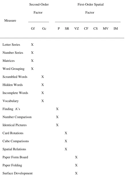
Hypothesised Factorial Structure of Test Battery
________________________________________________________________________
Second-Order First-Order Spatial
Factor Factor
Measure ____________ ______________________________________
Gf Gc P SR VZ CF CS MV IM
________________________________________________________________________
Letter Series X
Number Series X
Matrices X
Word Grouping X
Scrambled Words X
Hidden Words X
Incomplete Words X
Vocabulary X
Finding A’s X
Number Comparison X
Identical Pictures X
Card Rotations X
Cube Comparisons X
Spatial Relations X
Paper Form Board X
Paper Folding X
Surface Development X
________________________________________________________________________
Second-Order First-Order Spatial
Factor Factor
Measure ____________ ______________________________________
Gf Gc P SR VZ CF CS MV IM
________________________________________________________________________
Hidden Figures X
Hidden Patterns X
Copying X
Gestalt Completion X
Concealed Words X
Snowy Pictures X
Shape Memory X
Building Memory X
Map Memory X
Emergent Forms X
Transformation X
CAB-S Qnre X
Vandenberg Qnre X
Betts’ QMI X
Gordon’s TVIC X
Marks’ VVIQ X
________________________________________________________________________
Second-Order First-Order Spatial
Factor Factor
Measure ____________ ______________________________________
Gf Gc P SR VZ CF CS MV IM
________________________________________________________________________
Picture (RT) X
Add (NC) X
Subtract (NC) X
Rotation (NC & RT) X
Visual Memory (NC & RT) X
Line Memory (NC & RT) X
Dot Matrix (NC) X
________________________________________________________________________
Note. CAB-S Qnre = Dean and Morris (1995) questionnaire with the CAB-S shape;
Vandenberg Qnre = Dean and Morris (1995) questionnaire with the Vandenberg spatial shape;
NC = number correct (i.e., accuracy); RT = reaction time (mean latency).
In most respects, the design satisfied the main aims of the study in that it provided adequate opportunity for investigating the nature of visual imagery ability from an individual differences perspective. The design also enabled a test of the relationship between spatial ability and individual differences in visual imagery. The battery included traditional psychometric markers to identify the broad ability factor of Gv. This allowed for the proposed Imagery (IM) factor to be anchored against major spatial factors in the domain of visual perception: VZ, SR, CS, CF, P, and MV abilities.
Procedure
timed test battery of psychometric tests primarily taken from the 1976 ETS kit: Gf, Gc, P, SR, VZ, CF, CS, and MV. A short break was provided half way through each test session to help reduce fatigue. In the second test session, participants completed the series of self-report imagery questionnaires, the experimental measures of imagery ability, and finally the creative imagery tasks. Participants worked at their own pace in this final session. There were up to 12 people present at any one time during the first test session, with a maximum of five present during the second test session. Testing was completed over a 6 month period. Participants were provided with feedback on their imagery ability at the completion of the study.
Results
Preliminary Analyses
The aim of this stage of the analyses was to arrive at a set of reliable measures for inclusion in the factor analyses that were the main focus of this paper. In most cases, the preliminary analyses consisted of reliability checks and, where appropriate, slight modifications to tests to improve reliability. In other cases, however, exploratory factor analyses (EFA) were employed to determine the structure of variables whose construct validity was not clear from the literature. To this end, Principal Axis Factoring (PAF) was followed by direct Oblimin (oblique) procedures. Root one criterion, scree plots, and previous empirical findings were used to help determine the number of factors and, hence, the number of variables obtained from each measure. A summary of all modifications to variables is presented in point form below. No details are provided for variables where the factor structure was already clear and initial reliability estimates were satisfactory (see Table 2). The Method section provides an adequate description of these variables.
(a) The Matrices test (Gf3 marker variable) was reduced to a 10-item scale to improve reliability.
(b) The Hidden Figures test (CF1 marker variable), although not known as a particularly difficult test, had a very low mean (M = 3.56, SD = 2.21) in this sample, and demonstrated rather low reliability (α = .58). As noted earlier, the test was modified for the present study. The test was dropped from subsequent analyses.
(c) The QMI (vividness), TVIC (control), and VVIQ (vividness) questionnaires were each judged to be unidimensional.
(d) For the Dean and Morris (1995) imagery questionnaire, the CAB-S scale items loaded together to define a separate factor, correlated with but distinct from the factor defined by the Vandenberg scale items. Hence, those processes required to form images of two-dimensional and three-dimensional shapes appeared sufficiently different to warrant separate factor analyses of the two scales. The CAB-S and Vandenberg scales both showed evidence of a dominant first factor. Thus, two composite scale scores were obtained from the Dean and Morris questionnaire, each tapping a combination of imagery dimensions (e.g., ease of formation, detail, clarity, maintenance, vividness, ease of rotation, and control processes). A correlation of .63 (p < .01) was evident between these total scale measures, CABSqnre and Vandqnre, respectively.
.68, respectively), a composite measure (AddSubNC; variable 43) was computed. This variable provided a more reliable measure of image quality (α = .75).
The main aim of the next stage of data analysis was to investigate the
underlying structure of the test battery. This was done in stages, with each section of the battery analysed in turn. Confirmatory Factor Analysis (CFA) was used for sections of the battery where there were clear expectations about the structure, otherwise EFA was used. Structural Equation Modeling (SEM) was performed using the AMOS 3.6 (Arbuckle, 1997) computer package. PAF, with oblique rotation, from the SPSS package was used for EFA. Following the analyses of individual sections, the structure of the whole battery was analysed. Several indices of overall model fit were used for CFA. For present purposes, the Non-Normed Fit Index (NNFI) recommended by McDonald and Marsh (1990) and the Root Mean Square Error of Approximation (RMSEA) recommended by Browne and Cudeck (1993) were considered as well as the usual χ2 measure of goodness of fit. The χ2/df (i.e.,
minimum discrepancy:degrees of freedom) ratio provides information on the relative efficiency of the hypothetical model in accounting for the sample data. Values of 2.0 or less represent an adequate fit (Brookings, 1990; Byrne, 1989). The NNFI varies along a 0-1 continuum in which values greater than .9 are taken to reflect an
acceptable fit. Browne and Cudeck suggest that an RMSEA value below .05 indicates a close fit and that values up to .08 are still acceptable. The Comparative Fit Index (CFI) was also used.
Main Analyses
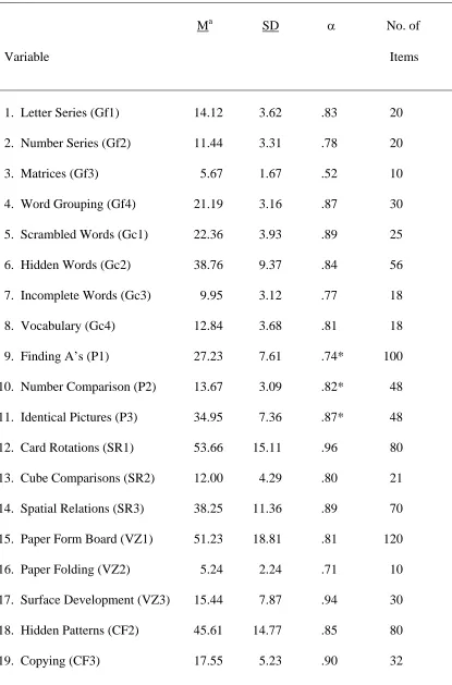
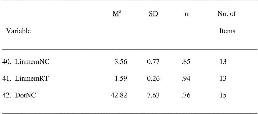
Table 2
Summary Statistics for All Variables
____________________________________________________________________________________
Ma SD α No. of
Variable Items
____________________________________________________________________________________
1. Letter Series (Gf1) 14.12 3.62 .83 20
2. Number Series (Gf2) 11.44 3.31 .78 20
3. Matrices (Gf3) 5.67 1.67 .52 10
4. Word Grouping (Gf4) 21.19 3.16 .87 30
5. Scrambled Words (Gc1) 22.36 3.93 .89 25
6. Hidden Words (Gc2) 38.76 9.37 .84 56
7. Incomplete Words (Gc3) 9.95 3.12 .77 18
8. Vocabulary (Gc4) 12.84 3.68 .81 18
9. Finding A’s (P1) 27.23 7.61 .74* 100
10. Number Comparison (P2) 13.67 3.09 .82* 48
11. Identical Pictures (P3) 34.95 7.36 .87* 48
12. Card Rotations (SR1) 53.66 15.11 .96 80
13. Cube Comparisons (SR2) 12.00 4.29 .80 21
14. Spatial Relations (SR3) 38.25 11.36 .89 70
15. Paper Form Board (VZ1) 51.23 18.81 .81 120
16. Paper Folding (VZ2) 5.24 2.24 .71 10 17. Surface Development (VZ3) 15.44 7.87 .94 30 18. Hidden Patterns (CF2) 45.61 14.77 .85 80
19. Copying (CF3) 17.55 5.23 .90 32
____________________________________________________________________________________
Ma SD α No. of
Variable Items
____________________________________________________________________________________
20. Gestalt Completion (CS1) 7.06 1.52 .85* 10
21. Concealed Words (CS2) 12.31 4.03 .83* 25
22. Snowy Pictures (CS3) 9.21 1.94 .68* 12
23. Shape Memory (MV1) 11.12 2.42 .68* 16
24. Building Memory (MV2) 9.13 2.47 .80* 12
25. Map Memory (MV3) 10.33 1.48 .77* 12
26. Emergent 9.61 4.50 .76 6
27. Transform 9.66 1.94 .79 12
28. CABSqnre 78.51 16.96 .87 13
29. Vandqnre 76.69 18.67 .90 13
30. QMI 193.38 26.97 .95 35
31. TVIC 9.91 2.32 .80 12
32. VVIQ 120.65 20.59 .95 32
33. PictureRT 1.50 0.18 .97 20
43. AddSubNC 11.79 4.32 .75 24
36. RotateNC 36.11 5.96 .86 50
37. RotateRT 1.36 0.16 .96 50
38. VismemNC 16.25 2.51 .65 20
39. VismemRT 1.23 0.13 .89 20
____________________________________________________________________________________
Ma SD α No. of
Variable Items
____________________________________________________________________________________
40. LinmemNC 3.56 0.77 .85 13
41. LinmemRT 1.59 0.26 .94 13
42. DotNC 42.82 7.63 .76 15
____________________________________________________________________________________
Note. * Alpha coefficients for speed tests provided in the 1976 ETS kit.
[image:21.595.86.514.103.293.2]RT = Log (10) of Reaction Time (in secs); NC = Number Correct. a N = 213.
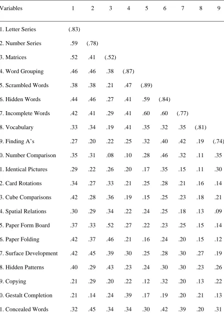
Table 3 presents the correlations obtained among all 41 variables. The latency measures (i.e., RT variables) have not been reflected. The reliability estimates
Table 3
Correlations Between All Variables
_____________________________________________________________________________
Variables 1 2 3 4 5 6 7 8 9
_____________________________________________________________________________ 1. Letter Series (.83)
2. Number Series .59 (.78)
3. Matrices .52 .41 (.52)
4. Word Grouping .46 .46 .38 (.87)
5. Scrambled Words .38 .38 .21 .47 (.89)
6. Hidden Words .44 .46 .27 .41 .59 (.84)
7. Incomplete Words .42 .41 .29 .41 .60 .60 (.77)
8. Vocabulary .33 .34 .19 .41 .35 .32 .35 (.81)
9. Finding A’s .27 .20 .22 .25 .32 .40 .42 .19 (.74)
10. Number Comparison .35 .31 .08 .10 .28 .46 .32 .11 .35
11. Identical Pictures .29 .22 .26 .20 .17 .35 .15 .11 .30
12. Card Rotations .34 .27 .33 .21 .25 .28 .21 .16 .14
13. Cube Comparisons .42 .28 .36 .19 .15 .25 .23 .18 .21
14. Spatial Relations .30 .29 .34 .22 .24 .25 .18 .13 .09
15. Paper Form Board .37 .33 .52 .27 .22 .23 .25 .15 .14
16. Paper Folding .42 .37 .46 .21 .16 .24 .20 .15 .12
17. Surface Development .42 .45 .39 .30 .25 .28 .30 .27 .19
18. Hidden Patterns .40 .29 .43 .23 .24 .30 .30 .23 .26
19. Copying .21 .29 .20 .22 .12 .32 .20 .13 .22
20. Gestalt Completion .21 .14 .24 .39 .17 .19 .20 .21 .13
21. Concealed Words .32 .45 .34 .34 .30 .42 .39 .20 .31
_____________________________________________________________________________
Variables 1 2 3 4 5 6 7 8 9
_____________________________________________________________________________ 22. Snowy Pictures .21 .16 .11 .29 .12 .19 .17 .15 .15
23. Shape Memory .37 .19 .30 .14 .13 .19 .23 .11 .16
24. Building Memory .35 .23 .29 .15 .13 .19 .23 .22 .15
25. Map Memory .25 .22 .22 .15 .20 .19 .13 .18 .16
26. Emergent .42 .31 .34 .38 .32 .32 .32 .26 .17
27. Transform .44 .42 .37 .42 .34 .30 .30 .37 .19
28. CABSqnre .25 .12 .20 .21 .15 .13 .14 .09 .10
29. Vandqnre .21 .16 .16 .20 .12 .11 .13 .15 .11
30. QMI .11 -.03 -.01 .04 .03 .04 .05 -.10 .06
31. TVIC .22 .24 .22 .19 .17 .17 .12 .23 .17
32. VVIQ .17 .07 .12 .04 .11 .03 .13 .03 .12
33. PictureRT -.08 -.02 -.07 -.04 -.03 .04 -.03 -.07 -.07
43. AddSubNC .39 .25 .31 .21 .20 .17 .29 .12 .15
36. RotateNC .14 .17 .09 .22 .20 .21 .18 .28 .08
37. RotateRT -.14 -.08 -.07 -.11 .06 .03 -.11 -.07 -.04
38. VismemNC .25 .17 .30 .03 .12 .21 .18 .00 .13
39. VismemRT -.15 -.09 -.17 -.15 .06 -.04 .06 -.02 -.10
40. LinmemNC .26 .18 .28 .15 .16 .13 .21 .16 .15
41. LinmemRT -.35 -.27 -.24 -.30 -.12 -.18 -.17 -.20 -.20
42. DotNC .31 .29 .30 .22 .21 .24 .23 .14 .19
_____________________________________________________________________________
Note. p < .05, r = .14. p < .01, r = .18.
_____________________________________________________________________________ Variables 10 11 12 13 14 15 16 17 18 _____________________________________________________________________________ 10. Number Comparison (.82)
11. Identical Pictures .34 (.87)
12. Card Rotations .14 .44 (.96)
13. Cube Comparisons .08 .45 .58 (.80)
14. Spatial Relations .09 .35 .77 .58 (.89)
15. Paper Form Board .04 .39 .55 .50 .55 (.81)
16. Paper Folding .01 .33 .46 .53 .50 .59 (.71)
17. Surface Development .04 .21 .40 .49 .42 .55 .57 (.94)
18. Hidden Patterns .18 .40 .37 .35 .30 .37 .26 .25 (.85)
19. Copying .28 .49 .39 .26 .28 .40 .31 .31 .28
20. Gestalt Completion .01 .14 .15 .15 .13 .22 .25 .32 .18
21. Concealed Words .29 .23 .14 .16 .12 .31 .23 .33 .23
22. Snowy Pictures .20 .21 .14 .17 .12 .14 .13 .09 .15
23. Shape Memory .11 .26 .27 .29 .25 .22 .21 .21 .38
24. Building Memory .16 .17 .14 .21 .12 .18 .17 .28 .26
25. Map Memory .12 .19 .26 .24 .27 .20 .18 .24 .17
26. Emergent .09 .25 .33 .30 .41 .40 .40 .39 .31
27. Transform .10 .24 .34 .34 .39 .41 .40 .49 .36
_____________________________________________________________________________ Variables 10 11 12 13 14 15 16 17 18 _____________________________________________________________________________ 28. CABSqnre .11 .13 .31 .28 .31 .23 .21 .17 .24
29. Vandqnre -.00 .06 .22 .28 .30 .20 .26 .30 .16
30. QMI .14 .17 .17 .17 .14 .09 .10 -.01 .07
31. TVIC .08 .20 .26 .22 .21 .18 .12 .17 .21
32. VVIQ .07 .06 .15 .12 .14 .13 .13 .13 .14
33. PictureRT -.03 -.12 -.23 -.19 -.18 -.16 -.12 -.02 -.04
43. AddSubNC .16 .17 .24 .22 .27 .24 .23 .30 .35
36. RotateNC .22 .14 .09 .11 .15 .11 .07 .29 .10
37. RotateRT .01 -.05 -.37 -.37 -.32 -.38 -.33 -.26 -.06
38. VismemNC .19 .25 .03 .16 .17 .14 .18 .09 .24
39. VismemRT -.08 -.14 -.29 -.25 -.32 -.12 -.17 -.06 -.11
40. LinmemNC .15 .32 .26 .23 .25 .32 .25 .25 .25
41. LinmemRT -.11 -.20 -.31 -.25 -.31 -.23 -.25 -.26 -.22
42. DotNC .27 .33 .28 .21 .26 .29 .23 .24 .34
_____________________________________________________________________________
_____________________________________________________________________________ Variables 19 20 21 22 23 24 25 26 27 _____________________________________________________________________________
19. Copying (.90)
20. Gestalt Completion .20 (.85)
21. Concealed Words .26 .30 (.83)
22. Snowy Pictures .09 .21 .10 (.68)
23. Shape Memory .14 .15 .11 .12 (.68)
24. Building Memory .12 .18 .07 .21 .37 (.80)
25. Map Memory .17 .13 .17 .05 .32 .37 (.77)
26. Emergent .28 .26 .16 .17 .36 .28 .19 (.76)
27. Transform .19 .29 .30 .26 .26 .34 .30 .45 (.79)
28. CABSqnre .19 .22 .03 .05 .31 .16 .23 .32 .20
29. Vandqnre .13 .17 .10 .03 .27 .23 .14 .36 .27
30. QMI .15 .12 .05 -.01 .10 -.04 .06 .10 -.00
31. TVIC .19 .12 .19 .13 .16 .11 .17 .17 .25
32. VVIQ .09 .13 .04 -.04 .08 .09 .14 .12 .14
33. PictureRT -.11 -.19 -.07 .00 -.09 -.01 -.09 -.10 -.09
43. AddSubNC .13 .13 .08 .17 .39 .34 .14 .34 .38
36. RotateNC .09 .15 .13 .13 .04 .20 .11 .23 .35
37. RotateRT -.26 -.14 -.03 -.15 .01 .04 .03 -.25 -.16
38. VismemNC .04 .06 .13 .17 .27 .17 .10 .21 .15
39. VismemRT -.19 -.14 -.08 .02 .00 .06 -.04 -.10 -.06
40. LinmemNC .26 .25 .14 .24 .21 .12 -.04 .33 .27
41. LinmemRT -.18 -.13 -.07 -.20 -.22 -.18 -.11 -.28 -.23
42. DotNC .23 .15 .15 .16 .30 .22 .21 .34 .33
_____________________________________________________________________________ Variables 28 29 30 31 32 33 43 36 _____________________________________________________________________________
28. CABSqnre (.87)
29. Vandqnre .63 (.90)
30.QMI. .41 .30 (.95)
31. TVIC .37 .32 .34 (.80)
32.VVIQ .47 .34 .57 .32 (.95)
33. PictureRT -.31 -.26 -.29 -.25 -.28 (.97)
43.AddSubNC .22 .14 .01 .18 .03 .09 (.75)
36. RotateNC .16 .16 .09 .11 .08 -.02 .17 (.86)
37. RotateRT -.16 -.12 -.14 -.02 -.03 .25 .02 -.12
38. VismemNC .12 .11 .01 .16 .04 .10 .27 .15
39. VismemRT -.13 -.12 -.12 -.10 -.08 .20 .04 .19
40. LinmemNC .26 .19 .20 .16 .29 -.07 .28 .13
41. LinmemRT -.08 -.22 .03 -.13 -.08 .09 -.21 .02
42. DotNC .17 .11 .06 .11 .11 .01 .40 .13
_____________________________________________________________________________
________________________________________________________________
Variables 37 38 39 40 41 42
________________________________________________________________
37. RotateRT (.96)
38.VismemNC .09 (.65)
39. VismemRT .40 .22 (.89)
40. LinmemNC -.22 .19 -.09 (.85)
41. LinmemRT .08 -.03 .33 -.18 (.94)
42. DotNC -.11 .30 -.07 .36 -.15 (.76)
________________________________________________________________
Stage 1: Confirming the structure of the spatial reference variables.
The 17 spatial tests included as reference variables for the broad Gv factor were factor analysed using CFA to establish whether the hypothetical six-factor structure was obtained (see Table 1). According to this model, three markers acted as indicator variables for each of the five major spatial primaries: VZ, SR, CS, P, and MV factors. Only two markers were included as indicator variables for the CF factor, given that the Hidden Figures test (CF1) was earlier removed from the battery because of poor reliability. A satisfactory fit was not obtained for the six-factor model (unreported) due to a problem with negative variance of the CF factor. Closer inspection of the correlation matrix reported in Table 3 indicated that the remaining marker tests for the CF factor were substantially correlated with other spatial marker variables, including those of factor P. Both these spatial primaries are thought to tap speed processes involved in the visual search and comparison of simple figural designs.
EFA, using PAF with oblique rotation, was introduced at this point to help determine the structure of the spatial reference battery. The pattern matrix
factors. The two CF variables and the three P variables acted as indicator variables for a combined P/CF factor. The five traits were again allowed to be correlated. Finally, the second-order Gv factor was extracted from analysis of the five first-order spatial factors. Table 4 presents the results of the CFA of the revised model for the 17 reference spatial variables.
Standardised AMOS Parameter Estimates for the Gv Reference Variable First-Order and
Second-Order Models
___________________________________________________________________________
First-Order Second-Order
Factor Factor
_______________________________ _____________
Variable P/CF CS SR VZ MV Gv
__________________________________________________________________________ First-Stratum Factor Loadings
9. Finding A’s .437
10. Number Comparison .424
11. Identical Pictures .738
18. Hidden Patterns .566
19. Copying .613
20. Gestalt Completion .480
21. Concealed Words .598
22. Snowy Pictures .279
12. Card Rotations .870
13. Cube Comparisons .700
14. Spatial Relations .862
15. Paper Form Board .796
16. Paper Folding .747
17. Surface Development .715
23. Shape Memory .612
24. Building Memory .591
25. Map Memory .581
__________________________________________________________________________
First-Order Second-Order
Factor Factor
_______________________________ _____________
Variable P/CF CS SR VZ MV Gv
__________________________________________________________________________
Factor Correlation Matrix
P/CF 1.00
CS .65 1.00
SR .60 .32 1.00
VZ .58 .65 .77 1.00
MV .52 .43 .45 .46 1.00
Second-Stratum Factor Loadings
P/CF .717
CS .645
SR .815
VZ .907
MV .560
__________________________________________________________________________
Note. p < .01, r = .32.
The CFA of the spatial test data showed that the revised five-factor oblique model provided a satisfactory fit to the data (χ2 = 200.452, df = 109, p < .001; χ2/df ratio = 1.839, RMSEA = .063, NNFI = .894, and CFI = .915). The interfactor correlations were quite large (ranging from .32 to .77), reflecting the “positive
recent studies of abilities in the domain of visual perception (e.g., Carroll, 1993; Lohman et al., 1987), VZ had the highest loading on the Gv factor.
In sum, a five-factor oblique model with latent dimensions corresponding to VZ, SR, MV, CS, and P/CF spatial primaries was established. In addition, a model hypothesising a second-order Gv factor was fitted to the data. The reference variables, with the exception of the combined P/CF factor, provided the expected structure against which to evaluate the structure of the visual imagery variables.
Stage 2: Confirming the structure of the visual imagery variables. The following analyses were directed at investigating the structure of the
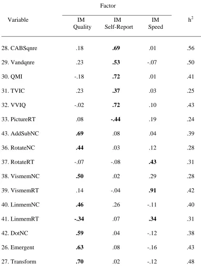
Table 5
Factor Loadings, Communalities (h2), and Percents of Variance for PAF Analysis
with Oblique Rotation on Imagery Variables
__________________________________________________________________
Factor
____________________________________
Variable IM IM IM h2
Quality Self-Report Speed
__________________________________________________________________
28. CABSqnre .18 .69 .01 .56
29. Vandqnre .23 .53 -.07 .50
30. QMI -.18 .72 .01 .41
31. TVIC .23 .37 .03 .25
32. VVIQ -.02 .72 .10 .43
33. PictureRT .08 -.44 .19 .24
43. AddSubNC .69 .08 .04 .39
36. RotateNC .44 .03 .12 .28
37. RotateRT -.07 -.08 .43 .31
38. VismemNC .50 .02 .29 .28
39. VismemRT .14 -.04 .91 .42
40. LinmemNC .46 .26 -.11 .40
41. LinmemRT -.34 .07 .34 .31
42. DotNC .59 .04 -.12 .38
26. Emergent .63 .08 -.16 .43
27. Transform .70 .02 -.12 .48
__________________________________________________________________
Factor
____________________________________
Variable IM IM IM h2
Quality Self-Report Speed
__________________________________________________________________
Eigenvalue 4.27 2.18 1.59
Percent of Variance 26.7 13.6 10.0
Factor Correlation Matrix
IM Quality 1.00
IM Self-Report .27 1.00
IM Speed -.09 -.22 1.00
__________________________________________________________________
Note. IM = Imagery.
p < .01, r = .22.
As shown in Table 5, the first factor was defined as Imagery (IM) Quality, with the creative imagery task variables (i.e., Emergent and Transform) and NC variables derived from the experimental imagery tasks loading most highly on this factor. Together, these variables were designed to tap aspects of image quality: The ability to generate a mental image, add and/or subtract detail from the image, rotate, maintain, and transform the image in specified ways. The second factor was defined by the five Imagery (IM) Self-Report measures. The PictureRT variable also showed a
substantial loading on this second factor. It was reasonable to expect this finding, given that the Picture task provided a subjective measure of the time that participants required to form a mental image of a particular scene. The remaining three RT variables from the experimental imagery tasks loaded together to define the final Imagery (IM) Speed factor. This factor reflected the efficiency of those processes involved in the generation, maintenance, and transformation of mental
representations. The PictureRT and VismemNC variables also showed moderate loadings on the third factor, with the former used to define the IM Speed factor. The three imagery dimensions were not highly intercorrelated, although a moderate correlation (r = .27, p < .01) was evident between the IM Quality and IM Self-Report factors.
Stage 3: Investigating the status of the IM factors within the spatial domain.
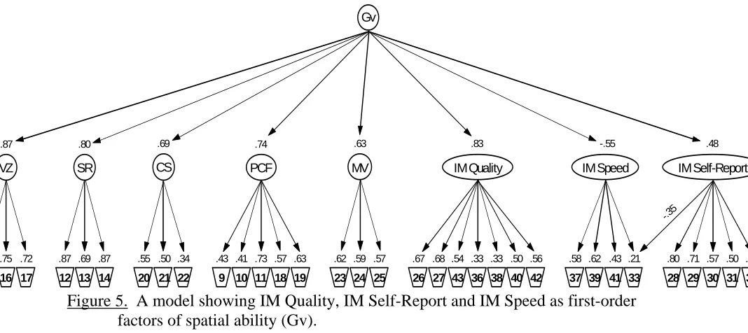
3.6 (Arbuckle, 1997). According to this eight-factor model, seven accuracy measures acted as indicator variables for the IM Quality factor, six introspective measures acted as indicator variables for the IM Self-Report factor, and four latency measures acted as indicator variables for the IM Speed factor. These 16 imagery variables were anchored against the five first-order spatial factors formerly presented in Table 4. Figure 5 presents the results of the CFA.
Figure 5. A model showing IM Quality, IM Self-Report and IM Speed as first-order factors of spatial ability (Gv).
A model with a second-order Gv factor provided a reasonable fit to the data (χ2 = 922.803, df = 487, p < .001; χ2/df ratio = 1.895, RMSEA = .065, NNFI = .780, and CFI = .799). The three hypothetical IM factors each showed substantial loadings (i.e., > .48) on the higher-order Gv factor. It should be noted that the fit statistics of the model presented in Figure 5 could be improved by allowing some of the error terms to covary. For example, modification indices suggested adding pathways between error terms for the following variables: QMI and VVIQ, SR and CS, VismemNC and IM Speed, and RotateNC and VismemRT. Indeed, adding these four covariance pathways can be theoretically justified and would improve the fit indices of the model to more acceptable levels (χ2 = 830.931, df = 483, p < .001; χ2/df ratio = 1.720, RMSEA = .058, NNFI = .822, and CFI = .804). However, this was not done. As reported in Figure 5, the fit statistics were deemed adequate, meeting at least the minimum requirements (Brookings, 1990; Browne & Cudeck, 1993; Byrne, 1989).
Exploratory analyses.
The confirmatory solution, as suggested by the hypotheses that drove this study, was presented in the preceding sections of this paper. It was shown that under these conditions, it is possible to extract three separate factors of imagery ability from the data. However, because this study was to some extent exploratory, it was
considered worthwhile to examine the results of an EFA of the imagery and spatial measures. The aim was to see whether or not the tasks would line up in a different
pattern if they were freed of the constraints of a CFA. To this end, the visual imagery and Gv reference variables presented in Figure 5 were subjected to EFA, using PAF with oblique rotation. A solution employing root-one criterion yielded nine factors, accounting for 62.4% of the total variance. Cattell’s (1966) scree test indicated that eight to nine factors might underlie the data. An eight-factor solution was computed to compare findings against those reported in the confirmatory model. The eight-factor solution (unreported) accounted for 59.1% of the variance, and was highly similar to the factor structure obtained by the CFA (see Figure 5).
The relationship between self-report imagery and spatial test measures. The second aim of this study was to examine the relationship between self-report measures of visual imagery and tests of spatial ability. It was argued that the Dean and Morris (1995) imagery questionnaire introduced more objectivity to the measurement of imagery ability, requiring participants to introspect on their imagery of spatial shapes. For example, a two-dimensional CAB-S spatial shape and a three-dimensional shape from the Vandenberg and Kuse (1978) test were used as the stimuli for imagining. In contrast, the items from the QMI and VVIQ scales provided purely subjective measures of visual imagery vividness for familiar scenes. As
previously shown in Table 3, the CABSqnre and Vandqnre variables derived from the Dean and Morris questionnaire showed significant correlations with the majority of the SR, VZ, and MV marker variables (.14 < r < .31). In contrast, the self-report measures of imagery for non-spatial shapes generally failed to correlate with the other, more objective, measurement techniques. The TVIC self-report measure was the only other subjective measure to share some variance with the tests of spatial ability (.11 < r < .26, p < .05).
The Finke et al. (1989) creative imagery tasks were expected to show
significant correlations with the tests of spatial ability. Indeed, inspection of Table 3 indicated that the correlations among the Emergent and Transform variables and the spatial test scores were as robust as any of the correlations among the spatial
primaries themselves. The data therefore suggested that the measures derived from the Finke et al. tasks might be treated as additional markers of spatial ability,
Discussion
The main aim of the current study was to examine the status of a hypothetical Imagery factor within the domain of visual perception. A wide range of visual
imagery measures was included in the battery. The set included experimental tasks previously used to measure imagery, new measures that were tried for the first time here, and traditional self-report measures. Factor analysis of the set of visual imagery markers yielded three clearly distinguishable dimensions. These factors were
interpreted as IM Quality, IM Self-Report, and IM Speed. Individual differences in the IM Quality factor were associated with variation in response accuracy, defined as the ability to generate, maintain, and transform a clear visual image. The self-report imagery questionnaires and PictureRT variable loaded together to define a separate factor, distinct from those factors defined by the more “objective” measurement techniques. These visual imagery questionnaires required participants to introspect on their ability to generate, control, and/or rotate a visual image. Finally, the IM Speed factor was interpreted as a reliable, separate dimension of individual differences in visual imagery ability, defined by the latency measures derived from the experimental tasks.
When included with a set of marker variables for well-replicated primary spatial abilities (Lohman et al., 1987), CFA methods indicated that the three Visual Imagery factors could be used as additional indicators for the broad Gv second order factor, alongside VZ, SR, CS, MV, and a combined P/CF factor. Each of the three Visual Imagery factors showed substantial loadings on this broad factor. It can therefore be argued that the IM Quality, IM Self-Report, and IM Speed factors can each be distinguished as constructs that give rise to individual differences in visual perception.
The results indicated that the three Visual Imagery factors can be located within the domain of spatial ability. As shown in Figure 5, IM Quality, IM Self-Report, and IM Speed are each conceived to be a primary factor of spatial ability. It is notable that the IM Quality factor shared considerable variance with each of the major spatial factors (.52 < r < .72). The IM Speed factor also showed moderate to strong correlations with the spatial primaries (.34 < r < .48). In contrast, the IM Self-Report factor emerged distinct from, yet related to, the level and speed factors defined by the more “objective” imagery measures. An issue that therefore needs addressing is the question of whether the IM Quality measures might best be envisaged as belonging to one of the other spatial primaries, rather than representing a separate factor of visual imagery ability.
linked to the mental synthesis and mental movement transformations posited by Lohman (1988) as being central to spatial test performance. It is therefore not surprising that the IM Quality factor showed significant intercorrelation with the VZ factor (r = .72). Nevertheless, it was shown that the processes required by the IM Quality factor are sufficiently different from the processes required by the major spatial primaries. The CFA results indicated that the IM Quality factor represents a separate factor that should not be subsumed under those factors well-replicated in the spatial ability domain.
An important finding of the present study is that the IM Self-Report factor emerged as a reliable dimension of individual differences in visual imagery ability, relatively independent of the other first-order spatial factors (.30 < r < .42). The imagery questionnaires typically require participants to introspect on the nature of a visual image, for example the vividness and/or ease with which an image can be controlled. The subjective experience of imagery can range from reports of no imagery at all, to clear, vivid images. The introspective measures were shown to be internally consistent and reliable and to load on a common imagery factor in both the exploratory and confirmatory solutions. The results also supported the convergent validity of the visual imagery scales. For example, the correlation of .32 between the TVIC self-report measure of visual imagery control and the VVIQ measure of
[image:38.595.92.503.451.707.2]imagery vividness was not as strong as the relationship of .57 between the VVIQ and QMI imagery vividness questionnaires. Such evidence of consistency within the self-report domain suggests that these ratings should not be dismissed as meaningless, even though they do not correlate as highly with objective measures of spatial abilities as some might expect.