The application of discounted cash flow for land development projects

The Application of Discounted Cash Flows for Land Development Projects By Shane Simmons, University of Southern Queensland

Abstract:Competition between property related professionals and demand by clients for increased service levels is causing greater demands to be placed upon the professional surveyor ill order to justify fee levels and maintain market share, relevance and professional standing. The surveying profession with a broad-based knowledge of property and spatial information is ideally placed to take advantage of opportunities in land development. The surveyor can value add land surveying services through knowledge and qualifications in project management, civil engineering, property analysis and environmental engineering etc.

This paper examines an aspect of property investment analysis methodology for determining the viability of potential land development projects developed over longer time frames whereby the time cost of money is included in the modelling process. Larger and more complex projects developed over longer timeframes require the consideration of the timing of cash flows and the time value of money as a Discounted Cash Flow Model.

1.0 Introduction

The importance of proper professional advice to clients can be emphasised by the following extract from Marler and Ferguson (1999).

Allegations of incorrect or poor advice are easy to make and difficult to defend. Our worst example is of a claim alleging poor advice to a land developer over a period of 12 months on a series of residential estates. The claim, which was really a series of claims on the various subdivisions, totalled $3.6 million... The matter had nothing to do with field surveying - it was about costs of development, advice on council requirements, alleged delays in approvals etc. The surveyor acted on verbal instructions and gave verbal advice to a developer whom he had known for some time ... But when the real estate market crashed and the developer faced insolvency, friendship and ethics went out the window. We cannot over emphasise the importance of proper office procedures and records as the only means of defence ...

Discounted Cash Flow analysis is a form of financial analysis where a series of cash flows are projected over an extended period of time for which a number of measures of financial return are calculated and used for project evaluation.

The discounted cash flow (DCF) methodology interprets future cash flows of income and costs for an extended specified time period (usually over a number of years). Future cash flows are discounted back to the present to determine a present value or worth for the investment at a required risk-adjusted rate of return. Costs and income are considered over more than one period of time and 'because the worth of cash over time changes, it is necessary to discount the future cash to compare it with present cash', (Boyd).

The process of discounting is the reverse of compounding interest rates and allows a calculation of what a dollar in the future is worth right now based on the formula, PV

=

(1:~)"

,where PV is the present value of an amount FV in the future at an interest rate r for a period n. A simple example is to work out the present value of receiving $1 in five year's time at an inflation rate of 3% (answer, 86.26 cents).

2.0 DCF Modelling

The DCF methodology requires periodic cash flows of income and costs to be forecast over the life of a project, discounted at the investors required rate of return to arrive at a net present value to be incorporated into decision criteria for the possibility of project viability. Hence there are two distinct processes, accurately portraying the cash flows and deriving the discount rate.

A DCF model forecasts costs and income over a period, applying a reversion technique of costs and income over the term of the model thus conveniently calculating costs and income as a series of net cash flows presented as a Net Present Value (NPV) figure of today' s dollar.

In order to undertake a DCF appraisal for a land development project then an innate understanding of the following aspects of land development are required:

• development stages from start to completion or disposal

• tImmg and cost of development stages from proposal to development/construction to marketing and disposal

• professional/government charges and fees • utility connection charges ,

• marketing costs and periods for sale of land

• potential income from sale of subdivided lots over a selling period in order to dispose of all properties

• growth rate or variation in cost/fee structures over time • investors required rate of return

Once all costs and income are derived, the net cash flows represent the best estimate of the costs and income generated by a property over the term of the model.

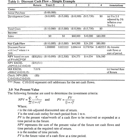
Table 1: Discount Cash Flow - Simple E:xample

Return Years 0 1 2 3 4 Annotations

Costs:

Initial Pun.:hasc ($100,000)

Development Costs ($10,000) (SI5,000) ($10,500) ($15.750) $0 (a) Yrs 2-3 adjusted by 5% inflation over Yrs 0-1 TOlal Costs (SIIO.OOO) ($15.000) ($10,500) (515.750) $0

Income:

Sales $0

so

$60,000 S40,000 S80.000

Net Cash Flow ($110,000) ($15,000) $49,500 $24,250 $80,000

Discount Factor 1.000000 0.833333 0.694444 0.578704 0.482253 (b) Assume

::: I/( I

+rt

where r ::: cash flows at

20Ck star! of period.

NPV based on sum ($35,511) ($110,000) ($12,500) $34,375 $14.034 $38,580 of PV=NCF*DF

NPV EXCEL ($35,511) ::=NPV(0.2,C JO:G 10)

IRR EXCEL 7.0 19c (c) Internal Rate

=IRR( C 1 O:G 10,15) of Return

Check: NPV(IRR( ($0) CIO:G 10),CI0:G 10)

***

Note: ClO:G 10 represent cell addresses for the net cash flows.

3.0 Net Present Value

The following formulae are used to determine the investment criteria:

NPV =

~

Y; and PV =

~F_V:--f:r

(1

+

r)"

(1

+

r)"

Where;

r is the risk-adjusted discounted rate of return. Y is the total cash outlay for each period from I to n.

PV is the present value/worth of a cash flow to be received or expended at a time period in the future.

NPV represents the sum of the present value of the future net cash flows and time periods at the required rate of return.

n is the number of time periods. "

FV is the future value of a cash flow at a time period.

A DCF model requires the documenting of cash flow projections over the period of the model such that future cash flows can be discounted back to their present value. When the present values of all cash flows in the model are summed the resulting figure is the Net Present Value (NPV) representing the present value of all cash flows in the model.

The NPV is best calculated "either by the NPV function of spreadsheet programs such as EXCELTM or electronic,calculation by either calculator (eg HP 48's) or computer

[image:4.630.75.563.61.590.2]

"~

If one required a static model with no consideration for the time cost of money then the discount rate would be treated as zero percent.

\

The decision criteria are relatively straightforward, if NPV is positive or equal to zero then accept project viability (unless other decision criteria disqualify viability). If a negative value is returned, then either reject the project viability or review the required rate of return and reassess the DCF model.

3.1 The Discount Rate

The required/expected or desired rate of return for an investment is determined by the discount rate representing a risk-adjusted rate of return. The discount rate normally includes a risk-free element plus specific risk elements.

Discount Rate

=

Risk-free rate

+

Specific risk rate

The risk-free element is normally the '10 year Commonwealth Bond Rate' and may include an allowance for inflation through including the Consumer Price Index rate.

Specific risk elements relate to macro-economic risk of the property market in general, micro-economic risk of the property or project individually and the investor's desired profit/risk factor for investing and risking funds.

In determining an appropriate discount rate for investment project's, the minImUm rate should at least reflect the '10 year Commonwe~lth Bond Rate' (which is normally considered a risk-free investment) otherwise the investor should place funds at the' 10 year' rate and forget about the project.

As an example let us sayan investor, wants to beat inflation (say 3%) and a risk-free rate (say 6%), and requires a decent return or profit margin for risking funds (say

16%). An appropriate discount rate may be the addition of those rates to determine

II

the investor's required rate of return to be a 25% discount rate.

The discount rate should not include the costs of financing the project or any taxation implications. The discount rate should reflect a nominal, un-geared (no finance) and before tax rate, as the objective is to assess project viability not a personal investor's financial status in conjunction with the project as well. Investor specific factors such as financing and taxation could be included but are best left in the realm of the investor's decision making process. If a personal investor wished to include the cost of financing then that could be reflected in the profit and risk factor they have provided.

An important consideration for the discount rate relates to whether cash flows are considered expended either at the beginning of a period or at the end of a period. It is possible to expend cash flows in the middle of the period, although that would be unusual but could be used to depict an average situation. The consideration of .the time period can have a major impact on the perceived financial return for the project.

,I

(

I

II

!

Note the change of the NPV in Table 2 from Table 1. The DCF model is deemed to commence at the initial purchase date and is allocated as time period 0 and cash flows are normally discounted from time period 1.

Table 2: Cash flows expended at beginning of period from Table 1.

Net Cash Flows ($110.000) $15,000 $~9,500 $24,250 $80,000

Discount Factor = 20% End Yr 0 0.8333333 0.69.t.t44 O.S7870~ 0.482253 OA01878

=

0.8333

(d) Cash flows treated at

end of period NPV ($29,593) ($91.667) ($ 100417) S28,646 $11.695 532,150

NPV EXCEL (S29.593) =NPV(0.2.D I O:G IO)+C I 0

Note: It is customary that the initial period of purchase is denoted time period 0 and the first discounted period is denoted time period 1.

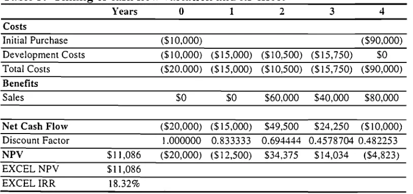
The effect of the timing of cash flows can be critical. Note the change in the NPV in Table 3 from Table 1 by considering' the initial purchase price as a deposit and balance on completion. Obviously deferring major costs and bringing forward income will enhance project viability.

Table 3: Timing of cash flow variation and its effect

Years 0 1 2 3 4

Costs

Initial Purchase (S I 0,000) ($90,000)

Development Costs (SIO,OOO) ($15,000) (SIO,500) (515,750) SO Total Costs (S20.000) (SI5,000) ($10,500) ($15,750) (S90,000) Benefits

Sales SO SO S60,000 S40,000 S80,000

Net Cash Flow Discount Factor (S20,000) 1.000000 (SI5,000) 0.833333 $49,500 0.694444 S24,250 0.4578704 (SIO,OOO) 0.482253 NPV SII,086 (S20,000) ($12,500) S34,375 S14,034 (S4,823) EXCEL NPV SII,086

EXCELIRR 18.32%

The major concern with using NPV is the requirement to have an appropriate discounted rate of return and that the adopted rate will most likely produce either a residual positive or negative NPV figure that may cloud the decision criteria. The NPV figure represents a profit or loss figure above or below the required rate of return for the investment. The existence of a residual value fails to indicate a calculated rate of return for the investment. For example, a 20% discount rate on a project with an average investment capital figure of $200,000 per time period with a positive residual NPV of $20,000, then what is the rate of return for the project? Answer ­ unknown as more calculations are required. The solution to the above problem is to calculate the internal rate of return (lRR)•.

I

IIII

I

[image:6.621.96.502.370.561.2]

4.0 Internal Rate of Return

The internal rate of return (IRR) calculates the rate of return based on the cash flows such that the NPV is zero. The IRR is the calculated rate of return that discounts the cash flows to a net sum of zero.

'

! .

II

The treatment of time periods (NPV calculated based on either beginning or end of a

I

period) does not dramatically affect the IRR as the NPV is multiplied by the discount rate increasing positive values and negative values accordingly resulting in similar

IRR's. Consequently calculating the NPV, best evidences the treatment of time periods and the resultant effect.

In essence, the IRR converts the cash flows to the rate of return at simple interest on the investment capital in the project where positive cash flows are assumed to retire debt in the project. A direct comparison can be made to the investor's required rate of return for an investment thus if the internal rate of return is greater than the investor's minimum required return then there is obviously a greater chance of the project proceeding. The investor's minimum required rate of return should be derived similarly to the discount rate.

Unfortunately the IRR is not easy to calculate manually and is generally based on an iterative procedure where both a negative and positive NPV figure are required at certain rates of return. The closer the figures are to zero (above and below) then the more accurate the calculation is for the IRR.

NPV/(}Irerruze (H' I R )] L R IRR =: X 19 lerRate - Lo'rver ate

+

ower ate

[ NPV/t1I.errllIe - NPV"ixherrme

Where higher and lower rates represent rates that return a positive and negative net present value respectively.

Table 4: Internal rate of return calculation

Net Cash Flow ($110,000) $15.000 $49,500 $24.250 $80,000

8.0090 Discount Factor =1/(1 +rl' 1.000000 0.925926 0.8573390.7938320.735030

NPV based on sum of ($3,396) (S)IO,OOO) ($13.889) $42.438 $19,250 $58,802 PV=DIO*DII

6.00lk. Discount Factor 1.000000 0.943396 0.8899960.8396190.792094

~~----~~~

NPV $3,427 (SIIO.OOO) (514.151) $44.055 S10.361 S63,367

-

IRR EXCEL =IRR(DIO:HIO, 15) 7.019c

I

ManualIRR 7.04lk.

I

The difference in the above manual calculation from the EXCELnl calculation relates

to the iterations used and non-linearity of manual calculation. The manual formula calculation in Table 4is based on NPV's of 8.00% and 6.00%.

There is the possibility of multiple solutions with the lRR as with each change of sign of cash flows inside the model there exists the same number of rates of return that satisfy the lRR formula. Normally the alternative solutions may be extreme and careful practicing professionals should spot the extreme alternative solutions by inspection of the cash flows.

Using the lRR function in a spreadsheet will not give you the 'average investment capital' for the project or the capital invested in the project at any time period. Consequently you get a rate of return figure but no indication of the investment or equity in the project at the various time periods. Both the lRR and NPV although based on compounding rate formulae are not strictly compounding rate based, as

...- positive cash flows are not reinvested for the term of the mode1.

The capital invested in a project is based on a mortgage table where costs are new borrowing's (added to the principal) and income retires debt (subtracted from the principal) with interest credited regularly based on the principal at that time. If required, the amount of capital invested in the project at a time period could be calculated using spreadsheet formulae or a macro function. In which case you would also probably provide a financial exposure row or column as a running total of the cash flows.

order to overcome the possibility of multiple solutions a modified internal rate of return can be used.

5.0 lVlodified Internal Rate of Return

The above methods do not consider the fact that positive cash flows or income can generate income rather than retire debt. The calculation of NPV and lRR, does not consider that negative cash flows and positive cash flows may have different rates of return (the holding cost of capital versus the reinvestment rate). In other words the cost of holding capital for expenditure may be different to the returns generated by positive cash flows or income: Note - the treatment of time periods for negative and positive cash flows are normally considered to be either at the beginning or at the end of the period, there is no flexibility with their treatment using EXCELTM NPVor lRR,

[image:8.609.87.541.71.206.2]

To modify the internal rate of return to account for the cost of holding capital involves discounting all negative cash flows to today's value or present value at the holding cost of capital. Note - this is not the interest rate for borrowed capital as interest costs if included could be expended as a cost in the cash flows, if not reflected in the investor's benchmark rate of return. All positive cash flows are projected forward to a future value at the end of the model at the appropriate reinvestment rate.

The modified internal rate of return is the rate of return that the total present value accumulates to the total future value. This calculates the rate of return of an initial outlay growing at a rate sufficient to cover all costs to a future value where positive cash flows generated during a project are invested at an appropriate rate until such time as the model is forecasting or the project is completed.

However there are two concerns in using the modified internal rate of return:

• What are the appropriate rates of holding capital and reinvesting capital? • How do we treat the time periods for negative and positive cash flows In

regressing and projecting cash flows respectively?

First of all we need to look at how any prudent and conservative developer would approach the development. The financial process would initially require securing capital to cover development costs to be held in a safe place whilst awaiting expenditure. Positive cash flows would either be re-invested or used to retire debt. So what are the appropriate rates?

The most likely holding place would be in a Cash Management Fund operated by a sound financial institution. Consequently the holding cost of capital or discount rate for negative cash flows is the current cash management rate (erring on the conservative side and sometimes including a risk-avoidance rate).

Reinvested cash flows should be considered to be either in a risk free environment and the safest capital investment is the '10 year' Commonwealth Bond Rate or utilised to retire debt in which case the rate would be the financing rate. It would be preferred not to utilise the financing rate as again that is the investor's personal consideration.

Changes in rates during the life of the project will obviously impact on the rate of return.

How do we treat time periods?

5.1 Calculating the Modified Internal Rate of Return

There is a modified internal rate of return function (MIRR) in EXCELn,t. the formula as expressed in the HELP menu is misleading in the treatment of time periods however the correct answer is calculated.

Although there is no specific function in EXCELTM to calculate net future values for a

series of cash flows, it is relatively simple to create spreadsheet formulae to perform the calculation. The advantage of doing your own calculation lies in the fact that you will have a start point figure indicating funding required and an end point figure indicating potential return generated. The client can then compare the potential return against their required rate of return that could include their personal investor consideration for profit/risk/financing and tax issues.

All negative cash flows are brought back to a present value at the cash management rate and all positive cash flows are carried forward to a future value at the required rate. This will give you the required start and end point figures. Then utilising compound interest formulae a rate of return can be calculated.

In the treatment of time for costs and income it is simply sound economics that if you money is owed to you then payment is required as soon as possible or up-front and if money is owed by you then payment will be delayed as late as possible.

If the rates for holding capital and reinvesting capital are the same and time periods are treated the same then the MIRR will calculate to be the same as the IRR.

Table 5: Discount Cash Flow - Modified Internal Rate of Return

Years 0 1 2 3 ..t

Costs

Initial Purchase ($100,000)

Development Costs (SIO,OOO) (SI5,000) (SI0,500) (SI5,750) $0 Total costs ($110,000) (SI5,000) (SI0,500) ($15,750) $0 Income

Sales SO SO S60,000 S40,000 $80,000

Net Cash Flow ($110,000) (SI5,000) $49,500 S24,250 $80,000

4.0090 Present value of negative (SIIO,Ooo) ($14,423) cash flows

6.00% Future value of positive cash S55,618 S25,705 $80,000 flows

Total present value required $124,423 for funding

Total future value of $161,323 reinvested funds

Compounded Rate of Return 6.719c on Funding' .

[image:10.616.105.550.417.687.2]

-The modified internal rate of return allows for reinvestment of positive cash flows at a specified rate (preferably risk-free) and allows for the accumulation of funds (preferably at a risk-free rate or 'at-call' rate) to meet future outlays. The modified internal rate of return is the rate of interest that compQunds the present value of all future outlays to equate to the future value of all positive cash flows being reinvested for the remaining term of the model. In my view this is the most effective method of forecasting the viability of a project in conjunction with calculating the NPV.

6.0 Analysis

Because a DCF model involves extended periods, certain assumptions, a number of variables and growth rates in variables, any model developed requires sensitivity and scenario analysis.

Sensitivity analysis entails changing a range of variables by varying amounts generally on a scale basis, measuring the effect and documenting results on the returns for the model. Properly conducted sensitivity analysis will highlight the critical variables in the model. Scenario analysis considers several scenarios for the project on a 'worst' case basis to a 'best' case basis, This will provide a range of returns for what may be the worst outcome to the best outcome.

6.1 Surveyor/Client Scenario

The typical case for a surveyor requiring a DCF model would be when a client walks through the door and wants to subdivide land that the client already owns. I would expect that larger land developers would have the capacity to undertake their own financial analysis of project viability.

In the case of a client requiring staged development on land already owned then project viability is sustained if either the NPV is greater than zero at the required rate of return or NPV equals zero and the modified internal rate of 'return exceeds the investors required rate of return. Both measures of return should be documented as a check on calculations and allow comparison of returns.

6.2 Forecasting

The major criticism with DCF modelling is the reliance on forecasting a number of variables and the accuracy of that forecasting into the future. The more variables, the greater the possibility for error in interpretation. Obviously any major changes in any variables may severely impact on the measure of return.

Constant growth variables are normally assumed to escalate or grow at the inflation rate. Variables subject to market or economic forces require subjective judgement. Uncertainty of

"

I

II'

I

I

I

If the mo.del do.es net co.ver co.mplete dispo.sal o.f the property then a terminal value at the end o.f the mo.del must be determined fer the remaining life o.f the pro.perty 'in­ perpetuity' and disco.unted back to. the present. Mo.st exercises undertaken by the surveyo.r pro.bably will net require the calculatio.n o.f a terminal value which is normally based en capitalising the pro.perty at a market rate based en the annual

•

generated inco.me by the pro.perty and disco.unting that value back to. the present. Acquisitio.n and dispo.sal Co.sts sho.uld be inco.rpo.rated into. the respective cash flew fer purchasing o.r selling pro.perty.

Fer the surveYQr Qne Qf the mere difficult items to. Co.st wo.uld be the infrastructure charge. I suppo.se experience within each lo.cal autho.rity will o.ffer guidelines to. the

,

•

I

treatment o.f infrastructure charges as levied by the lo.cal autho.rity. infrastructure charge requires funding then the Co.st Qf funding sho.uld be inco.rpQrated If the into. the mo.del althQugh the difficulty lies with the interpretatiQn o.f the estimated amo.unt the lo.cal autho.rity will require. It wo.uld be critical to. discuss the interpretatio.n o.f infrastructure charges in the repo.rt.

7.0 DCF lVIodel Standards

..

As with any mo.del o.r precess ado.pted by any number o.f peo.ple o.r organisatio.ns then

•

I the use o.f that mo.del o.r process is enhanced if there is co.nsistency o.f repo.rting, termino.lo.gy, and presentatio.n. The fo.llo.wing requirements I believe are the minimum repo.rting standards fer a DCF mo.del:

~

!

• S tate the rest perio.d o.f time

• State the disco.unt rate

• Include all relevant Co.sts and inco.me

• Separate headings fer different cash flews.

• Medel based Qn a befo.re interest and tax basis and stated to. that effect

• The first periQd disco.unted be termed 1

• Checking mechanism fer measures o.f return

• Growth rates in variables fer time perio.ds at the inflatio.n rate unless

specifically co.mmented upo.n

The mo.del wo.uld net be co.mplete witho.ut being co.ntained in a repo.rt o.utlining the fo.llo.wing:

•

Purpo.se

I

•

Market and current eco.no.mic status discussio.n

I

,

I

•

Disco.unt rate discussio.n

•

Cash flQW discussio.n

-i

•

Rest periQd

•

Gro.wth rate in variables especially if net at the inflatio.n rate

•

Analysis discussio.n, especially sensitivity and scenario. analysis

•

Date produced

•

Autho.r

I

•

Pro.duct name and versio.n used fer creatio.n Qf DCF mQdel

•

Appro.priate limitatio.ns, qualifiers and disclaimer

I

Presentation can sometimes be a nightmare as any DCF model can become a multiple page document consequently a summary table should be included highlighting net cash flows, measures of financial return, possibly a chart of cash flow requirements and summary results of analysis.

8.0 Conclusion

The discount cash flow method is a valuable analysis tool for those evaluating potential investment decisions and in determining financial measures of return for a potential land development project. The modelling process can be created in 'Spreadsheet Programs' and once created can be applied for any new project after appropriate alterations.

References:

Boyd T.P, 1995, 'Property DCF's - What, Why, When, How ... But', The Valuer and Land Economist, AIVLE, August 1995, pp. 589-592.

Marler 1. and Ferguson R., 1999, 'Insurance', M&M - Measure and Map, July/August 1999, Issue 3, pp. 20-21.

Rowland PJ, 1997, Property InvestmeJlts and their Financing, Law Book Company, Sydney.

University of Queensland Publication's, 1997-9, Valuation Study Books, UQ, Brisbane.