Process Planning for Concurrent Multi-nozzle 3D Printing

Rochester Institute of Technology

RIT Scholar Works

Theses

4-19-2019

Process Planning for Concurrent Multi-nozzle 3D

Printing

Paritosh Santosh Mhatre

Follow this and additional works at:

https://scholarworks.rit.edu/theses

This Thesis is brought to you for free and open access by RIT Scholar Works. It has been accepted for inclusion in Theses by an authorized

Recommended Citation

PROCESS PLANNING FOR CONCURRENT

MULTI-NOZZLE 3D PRINTING

THESIS

Submitted to the

Department of Industrial & Systems Engineering

Kate Gleason College of Engineering

in Partial Fulfilment of the Requirements for the

Degree of

Master of Science in Industrial & Systems Engineering

Submitted by

PARITOSH SANTOSH MHATRE

Advisor

Dr. Denis Cormier

Earl W. Brinkman Professor, AMPrint Center Director

Committee Member

Dr. Marcos Esterman

Associate Professor

Rochester Institute of Technology

Rochester, NY

DEPARTMENT OF INDUSTRIAL & SYSTEMS ENGINEERING

KATE GLEASON COLLEGE OF ENGINEERING

ROCHESTER INSTITUTE OF TECHNOLOGY

ROCHESTER, NEW YORK

CERTIFICATE OF APPROVAL

APRIL 19, 2019

M.S. DEGREE THESIS

The M.S. Degree Thesis of Paritosh Mhatre

has been examined and approved by the

thesis committee as satisfactory for the

thesis requirement for the

Master of Science degree

Approved by:

Dr. Denis Cormier, Thesis Advisor

Earl W. Brinkman Professor, AMPrint Center Director

ABSTRACT

Additive manufacturing (AM) processes possess excellent capabilities for manufacturing complex

designs as single uniform parts with optimum material utilization. However, the processes are still not

widely used in industry to make large parts. The main reason for this slow adoption is the low material

deposition rate during printing. Increasing the material deposition rate by increasing the layer thickness or

utilizing larger diameter nozzles results in deterioration of the surface quality of the part. This is known as

the “staircase effect”; thus there is a trade-off between the print time and the surface finish of a part. A

majority of the research efforts focused on minimizing this trade-off aim to minimize the print time by

optimizing the layer thickness based on the evaluation of local geometry of the part. Another approach

adopted in minimizing this trade-off is to utilize multiple nozzles concurrently for increasing the material

deposition rate. The processes leveraging this approach use independent nozzles with relative motion

between them and are seen to be more suitable for parts with a large footprint in the X-Y plane. This thesis

further explores this direction of research by utilizing multiple nozzles, mounted on the same print-head,

for concurrent printing to increase the deposition rate. The algorithm developed here requires a rotational

axis. A 4-axis multi-nozzle toolpath generator, a G-code simulator and a proof-of-concept machine were

TABLE OF CONTENTS

ABSTRACT ……….……... I

LIST OF FIGURES ………... IV

LIST OF TABLES ………... VII

CHAPTER 1 INTRODUCTION ………... 1

1.1 THE TRADE-OFF ………... 1

1.2 THE STAUS-QUO ………... 2

1.3 MOTIVATION ...……….. ... 2

CHAPTER 2 LITERATURE REVIEW ………... 4

2.1 CLASSIFICATION OF ADAPTIVE SLICING PROCEDURES ……... 4

2.1.1 UNIFORM ADAPTIVE SLICING PROCEDURES ………... 5

2.1.2 DYNAMIC ADAPTIVE SLICING PROCEDURES ………... 6

2.2 MULTI-EXTRUDER SYSTEMS ………... 10

2.3 RESEARCH NEED ……….………... 11

2.4 THESIS STATEMENT ……….…………..………... 12

CHAPTER 3 METHODOLOGY ………..………... 13

3.1 NOZZLE CONFIGURATIONS ………... 13

3.2 ALGORITHM DEVELOPMENT………..………. 17

3.2.1 PRINT HEAD OR PLATFORM ROTATION ……….... 17

3.2.2 TOOLPATH PLANNING……… 22

3.2.3 NOZZLE ACTUATION ………... 30

3.2.4 RETRACTION ………. 33

3.3 SOFTWARE ………... 35

3.3.1 G-CODE GENERATION ……… 35

3.3.2 SLICER ………... 37

3.3.3 FIRMWARE ………. 39

3.4.2 EXTRUDER SYSTEM ………... 43

3.4.3 CONTROLLER ………... 44

3.5 PROCESS MAP ………. 44

CHAPTER 4 ANALYSIS & OBSERVATIONS ..………...………... 46

4.1 PROCESS ANALYSIS ….………. 46

4.2 OBSERVATIONS ………..…………...………..………... 48

4.3 PRINT RESULTS ..……… 49

4.3.1 2-NOZZLE 1D LINEAR CONFIGURATION ……… 50

4.3.2 4-NOZZLE POLYGON CONFIGURATION ………. 51

CHAPTER 5 DISCUSSION & FUTURE WORK………...………... 54

5.1 DISCUSSION ………. 54

5.2 FUTURE WORK ………...……… 55

5.2.1 BI-DIRECTIONAL PRINTING ………...………... 55

5.2.2 ADDITIONAL INFILL PATTERNS ………...………... 55

5.2.3 PRINT ORIENTATION ………...……….………... 55

5.2.4 NOZZLE UTILIZATION …………..………...………... 56

5.2.5 VARIABLE NOZZLES ..………... 56

5.2.6 MULTI-MATERIAL ……… 56

APPENDIX I –ACTUATION POINTS ………. 57

APPENDIX II – POST-PROCESSING SCRIPT ...………...………...………... 58

APPENDIX III – G-CODE SIMULATOR ………..………...……… 100

APPENDIX IV - TOOLPATH SIMULATION FOR LINEAR ARRAY, RECTILINEAR INFILL . 106 APPENDIX V - TOOLPATH SIMULATION FOR LINEAR ARRAY, CONCENTRIC INFILL ... 107

APPENDIX VI - TOOLPATH SIMULATION FOR POLYGON ARRAY, RECTILINEAR INFILL ... 108

APPENDIX VII - TOOLPATH SIMULATION FOR POLYGON ARRAY, CONCENTRIC INFILL .. 109

LIST OF FIGURES

FIGURE 1: CUSP HEIGHT ... 5

FIGURE 2: VARIABLE THICKNESSES FOR THE INTERIOR AND EXTERIOR REGIONS. ADAPTED FROM SABOURIN, HOUSER, AND HELGE BØHN 1997 ... 7

FIGURE 3: RAS VS TRADITIONAL ADAPTIVE SLICING. ADAPTED FROM MANI, KULKARNI, AND DUTTA 1999 ... 8

FIGURE 4: DEFINITION OF DIFFERENCE VOLUME. ADAPTED FROM YANG ET AL. 2003... 9

FIGURE 5: DUAL-NOZZLE EXTRUDER. ADAPTED FROM ALI, MIR-NASIRI, AND KO 2016 .... 10

FIGURE 6: 1-D LINEAR MULTI-NOZZLE ARRAY ... 13

FIGURE 7: OVER-TRAVEL REQUIRED BY MULTI-NOZZLE ARRAY ... 14

FIGURE 8: 2-D LINEAR MULTI-NOZZLE ARRAY ... 14

FIGURE 9: 2-D TRANSFORMED LINEAR MULTI-NOZZLE ARRAY ... 14

FIGURE 10: 3-NOZZLE POLYGON ARRAY ... 15

FIGURE 11: 4-NOZZLE POLYGON ARRAY ... 15

FIGURE 12: PRINT DIRECTIONS FOR A 3-NOZZLE POLYGON ARRAY ... 16

FIGURE 13: PRINT DIRECTIONS FOR A 4-NOZZLE POLYGON ARRAY ... 16

FIGURE 14: DERIVING ANGLES FOR FEASIBLE PRINTING DIRECTIONS ... 17

FIGURE 15: VARIABLE PRINTED LINE SPACING ACHIEVED WITH ROTATION OF A 1D ARRAY OF NOZZLES ... 19

FIGURE 16: VARIABLE OFFSET ACHIEVED WITH MULTIPLE PASSES FOR A POLYGON CONFIGURATION ... 20

FIGURE 17: 4-AXIS 3D PRINTER ... 22

FIGURE 18: TOOLPATH FOR A LAYER ... 23

FIGURE 21: ACTUATION POINTS FOR PERIMETER ... 24

FIGURE 22: PERIMETER TOOLPATH WITH 2 NOZZLES ... 25

FIGURE 23: 4 POINTS AT EACH VERTEX ... 26

FIGURE 24: RECTILINEAR INFILL ... 28

FIGURE 25: INFILL RAYS INTERSECTING WITH SQUARE PERIMETER ... 30

FIGURE 26: INFILL RAYS INTERSECTING WITH STAR PERIMETER ... 30

FIGURE 27: MOVING FROM VERTEX ‘I’ TO VERTEX ‘I+1’ ... 31

FIGURE 28: MOVING FROM VERTEX ‘I’ TO VERTEX ‘I+1’ FOR A SMALLER PART ... 32

FIGURE 29: ALGORITHM FLOWCHART ... 34

FIGURE 30: VERBOSE 3-AXIS G-CODE ... 38

FIGURE 31: POST-PROCESSED 4-NOZZLE 4-AXIS G-CODE ... 39

FIGURE 32: MATLAB G-CODE SIMULATOR ... 40

FIGURE 33: BUILD PLATFORM MOUNT ASSEMBLY (SIDE VIEW) ... 41

FIGURE 34: BUILD PLATFORM ASSEMBLY (TOP VIEW, CIRCULAR BUILD PLATE SET TO TRANSPARENT) ... 42

FIGURE 35: 2-NOZZLE 1-D LINEAR CONFIGURATION ... 43

FIGURE 36: 4-NOZZLE POLYGON CONFIGURATION ... 43

FIGURE 37: HOT-END SUPPORT FIXTURE: DESIGN (LEFT) AND WITH HOT-END MOUNTED (RIGHT) ... 44

FIGURE 38: PROCESS MAP FOR THE DEVELOPED MULTI-NOZZLE CONCURRENT PRINTING ... 45

FIGURE 39: CAD MODEL (LEFT) AND STL FILE (RIGHT) FOR THE 25MM SQUARE ... 47

FIGURE 40: 3-AXIS TOOLPATH (LEFT) AND 4-AXIS 4-NOZZLE TOOLPATH (RIGHT) FOR 25MM SQUARE ... 47

FIGURE 41: RIP VS PRINT TIME ... 48

FIGURE 43: 4-AXIS 2-NOZZLE TOOLPATH (LEFT) AND PRINT RESULT (RIGHT) FOR THE

SQUARE... 51

FIGURE 44: CAD MODEL (LEFT) AND STL FILE (RIGHT) FOR THE SPEAR SHAPED PART ... 52

FIGURE 45: 4-AXIS 2-NOZZLE TOOLPATH (LEFT) AND PRINT RESULT (RIGHT) FOR THE

LIST OF TABLES

TABLE 1: NOZZLE ACTUATION ... 31

TABLE 2: NOZZLE ACTUATION FOR SMALLER PARTS ... 32

TABLE 3: STANDARD G-CODE COMMANDS ... 35

TABLE 4: CUSTOM G-CODE ADDITIONS ... 37

TABLE 5: PINION AND GEAR DIMENSIONS ... 42

CHAPTER 1

INTRODUCTION

Additive manufacturing (AM) processes, since their advent in 1980s, have shown great potential and

have been expected to revolutionize the manufacturing industry. The processes are particularly well suited

for manufacturing complex designs as a single part with optimum material utilization. AM processes have

proved excellent for prototyping purposes, enabling product design teams to experience the physical

realization of design iterations within a few hours of design completion, without the requirement of specific

tooling and set-ups; thus justifying the name –“rapid prototyping processes”.

1.1.

The field of AM has witnessed continuous research and development efforts over the years, a part of

which can be attributed to its popularity among hobbyists; with the Fused Filament Extrusion (FFE) process

being the most popular of all the AM processes. The Big Area Additive Manufacturing (BAAM) system

developed by Oak Ridge National Laboratory (Holshouser et al. 2013) and commercialized by Cincinnati

Inc. (Krassenstein 2015) significantly increases the deposition rate using a large diameter nozzle and a

single screw extruder. LSAM developed by Thermwood Corporation is another large-scale system which

combines additive and subtractive processes on independent gantries on the same machine. Despite these

efforts, the status quo of AM processes shows that they have not made the leap from being the rapid

prototyping processes to be the mainstream large-scale manufacturing processes. The main reasons for this

shortcoming arise from the process limitations such as the limited gamut of compatible materials and the

trade-off between print time and the surface finish or “staircase effect” of the concerned parts. For special

AM applications like multi-material or multi-color printing, the time spent for material change further slows

1.2.

The surface finish and print time for a part are both related to the layer thickness used during printing,

i.e. as the layer thickness increases, the print time decreases while the surface finish of the part deteriorates.

Multiple research efforts were undertaken to minimize this trade-off, viz. adaptive slicing techniques, which

slice the CAD model with variable slice thicknesses based on the local geometry of the part. Since only the

surface finish of the outer surface is of aesthetic importance, an extension of adaptive slicing also varies

print thickness within a layer. Specifically, exterior contours of the part are printed with thinner tracks for

better surface finish, while the infill regions are printed using the maximum allowable track thickness for

faster print time (Sabourin, Houser, and Helge Bøhn 1997). Another approach adopted to minimize this

trade-off is to increase the deposition rate in a layer using multiple extruders simultaneously. The concurrent

multi-extruder systems use independent extruders capable of moving relative to each other and are suitable

for large-scale parts. A more common application of multiple extruders is to minimize the miscellaneous,

or tool change, time spent towards changing the material, where a separate nozzle is dedicated for each of

the required materials. However, these systems often only utilize one of the multiple extruders at any given

instance.

1.3.

This thesis explores the potential of concurrently utilizing multiple nozzles mounted on the same

print-head in a Fused Filament Extrusion (FFE) 3D printer with no relative motion between them. The resulting

system with a compact arrangement of nozzles will help minimize the part size limitation of the concurrent

systems.

The remainder of this document is organized as follows. Chapter 2 reviews the Literature Work

related to adaptive slicing techniques followed by implementation of multiple extruders. Chapter 3 states

5 discusses the Analysis & Observations of the developed process. Chapter 6 proposes the Discussion &

CHAPTER 2

LITERATURE REVIEW

The trade-off between print time and the surface finish of a 3D printed part is one of the main reasons

for the slow adoption of additive manufacturing processes by the mainstream manufacturing industry. As

discussed earlier, both these factors are related to the user-specified layer thickness. Hence, the research

efforts to minimize this trade-off are primarily focused on optimizing the layer thickness by developing

adaptive slicing procedures. The adaptive slicing techniques determine the local layer thickness by

evaluating the curvature of the local geometry of the part against a user defined parameter, like maximum

allowable cusp height.

The following sections describe these slicing procedure techniques in detail. Previous research utilizing

multiple extruders are also discussed, thus identifying the opportunity of concurrent utilization of multiple

extruders for every layer.

2.1.

This thesis classifies the previously proposed adaptive slicing procedures into 2 categories as below.

1. Uniform Adaptive Slicing procedures

These procedures slice the entire part adaptively based on the local geometry of the part. Thus, one

entire layer has uniform layer thickness, i.e., the layer thickness for the part remains constant in X-Y plane

but can vary from layer to layer along the Z-axis.

2. Dynamic Adaptive Slicing procedures

These procedures divide the part model into two regions viz. the interior and the exterior. The interior

region is sliced adaptively with thinner print tracks for better surface finish. Thus, the layer thickness for

the part varies along Z-axis and may also vary in the X-Y plane.

2.1.1 UNIFORM ADAPTIVE SLICING PROCEDURES

As described earlier, this category describes the adaptive slicing procedures that result in uniform

thickness throughout an entire layer and variable layer thickness along the vertical build direction. The most

common user specified parameter utilized by adaptive slicing techniques to determine the layer thickness

is the maximum allowable cusp height, 𝐶𝑚𝑎𝑥 (Dolenc and Mäkelä 1994).

Figure 1: Cusp height

For each layer ′𝑛′, the thickness ′𝑡′ for layer ′𝑛 + 1′ is determined by the local geometry of the tessellated

CAD model, such that 𝑐 ≤ 𝐶𝑚𝑎𝑥, as shown in Figure 1. Thus, the surfaces of the model with high curvature

will have finer layer thickness, while the surfaces with lower curvature will have larger layer thickness. The

technique produces the smaller features of the part with faster print times, as compared to uniformly slicing

the entire part with very fine layer thickness.

Adaptive slicing using stepwise uniform refinement (Sabourin, Houser, and Helge Bøhn 1996) is a

technique based on a maximum allowable cusp height parameter. The method initially slices the tessellated

cusp height exceeds user specified maximum allowable cusp height (𝑐 > 𝐶𝑚𝑎𝑥), are further sliced

uniformly with finer thickness. The number of layers for this sub-division is determined using Equation 1.

𝛼𝑠𝑙𝑎𝑏= 𝑖𝑛𝑡 (

𝐿𝑚𝑎𝑥

𝐶𝑚𝑎𝑥

𝑚𝑎𝑥 {𝑛𝑧𝑏𝑜𝑡𝑡𝑜𝑚, 𝑛𝑧𝑡𝑜𝑝})

(1)

𝛼𝑠𝑙𝑎𝑏 ∈ [1, 𝛼𝑚𝑎𝑥], 𝛼𝑚𝑎𝑥 = 𝑖𝑛𝑡 ( 𝐿𝑚𝑎𝑥

𝐿𝑚𝑖𝑛)

where, 𝑛𝑧𝑏𝑜𝑡𝑡𝑜𝑚 𝑎𝑛𝑑 𝑛𝑧𝑡𝑜𝑝are the normal Z components for a point of a slab across the top and bottom slice.

This technique, as opposed to others, evaluates each slab along bottom-up and top-down directions, which

prevents missing any high curvature regions. Implementation of the technique on a Stratasys FDM 1600

rapid prototyping system resulted in a reduction in print time of approximately 50 percent, as compared to

a uniform layer thickness of 0.005 in.

The adaptive slicing techniques described above are based on a single user-specified maximum

allowable cusp height value which is applied to the entire CAD model. However, the surface finish

requirements for the users may vary for different surfaces of the same part, and hence the cusp height for

different surfaces should also vary accordingly. These requirements were captured by a slicing technique

(Cormier, Unnanon, and Sanii 2000) utilizing the user specified non-uniform cusp height for the different

surfaces of the tessellated CAD model. The technique takes an STL file as input and groups all the facets

belonging to the same face using an edge finding algorithm. The user specifies the required maximum

allowable cusp height for all the identified faces. The technique defines varying surface finish requirements

for different surfaces of a part before adaptively slicing it, thus reducing the print time further as compared

to techniques using a single user-specified cusp height value.

2.1.2 DYNAMIC ADAPTIVE SLICING PROCEDURES

These procedures first divide the CAD model or the tessellated CAD model into 2 regions, interior and

exterior and then apply an adaptive slicing technique to the exterior region and uniform maximum allowable

uniform adaptive slicing techniques discussed in section 2.1.1, but with faster print time. A user-specified

parameter like maximum allowable cusp height is employed here for determining the layer thickness of the

exterior region.

A slicing technique proposed for printing a part’s exterior surface accurately and the interior rapidly

(Sabourin, Houser, and Helge Bøhn 1997) first slices the STL model of the part into thick horizontal layers,

or ‘slabs’. The part is divided in interior and exterior regions by offsetting a contour obtained from the

intersection of the top and bottom contours of each ‘slab’. The exterior region is then sliced adaptively

using stepwise uniform refinement (Sabourin, Houser, and Helge Bøhn 1996), such that the uniform layer

thickness of the exterior layer is an integer fraction of the interior layer thickness. First, the exterior regions

are built using thin build layers; then the interior regions are backfilled as a single, fast, thick build layer to

complete the fabrication of the part within the slab as shown in Figure 2.

Figure 2: Variable thicknesses for the interior and exterior regions. Adapted from Sabourin, Houser, and

Helge Bøhn 1997

The approach implemented by the researchers using a Stratasys, Inc. FDM 1600 rapid prototyping

system resulted in an overall 50-80 percent reduction in print time of sample parts with dense interiors

without affecting the surface quality. The reduction in print time with this technique is more significant for

parts with dense interior, than parts with thin walls.

A Region-based Adaptive Slicing (RAS) technique (Mani, Kulkarni, and Dutta 1999) allows the users

RAS technique slices the ACIS.sat model at each vertex to ensure that any sharp feature is not missed. This

forms regions called ‘blocks’. Each ‘block’ is uniformly sliced with maximum permissible thickness to

form 2.5D regions called ‘zones’; which are further sub-divided into 2 regions: Region A, the Adaptive

Layer Thickness (ALT) region and Region C, the Common Interface Layer (CIL), as shown in Figure 3.

Figure 3: RAS vs traditional adaptive slicing. Adapted from Mani, Kulkarni, and Dutta 1999

The ALT outer region is sliced adaptively for better surface finish based on the user defined cusp height

for different surfaces, while the CIL inner region is sliced with the maximum thickness for faster

manufacture. For each zone, the top and bottom contours are projected on a common horizontal plane. The

inner and outer intersecting curves of this projection are offset by a positive and negative distance

respectively; with the positive offset being to the left and negative offset being to the right when moving

along the intersection curve in counter-clockwise (CCW) direction. The offset curves when extruded from

top to bottom of the zone form the parting surface, separating the CIL and ALT regions. Implementation of

RAS with a Stratasys FDM system has shown the technique to be beneficial in terms of print time reduction

primarily for model scaling factors over a cross-over point.

Another slicing technique (Ma and He 1999) utilizes adaptive slicing together with a selective hatching

strategy. It computes all the extreme points on the model surfaces to capture the peak features from a CAD

model based on non-uniform rational B-spline (NURBS) surfaces. The model is then sliced at these extreme

points to form slabs. Each of these slabs is further sliced with an adaptive slicing algorithm based on the

These can be defined separately for different layers. To minimize the trade-off between print time and

surface finish, this approach introduces a selective hatching strategy such that the skin regions are scanned

first for smooth surface finish. The internal areas are then scanned when the cumulative thickness of the

skin regions approaches the maximum allowable thickness of the process. The implementation of the

technique using Autodesk Mechanical Desktop software helped the authors achieve a 46% reduction in

print time over a traditional strategy.

All the slicing techniques described above utilize user-defined maximum allowable cusp height to

control the surface finish of a part. An adaptive slicing algorithm using a different criterion, called

successive layer area difference (SLAD) aims to minimize the volumetric difference between two adjacent

layers to overcome the inefficiency of the uniform cusp height criterion (Yang et al. 2003). The uniform

cusp height criterion can result in variability in the volumetric difference in different layers of the same

part. The volumetric difference varies significantly when the surface normal vector for the cusp is nearly

perpendicular to the layer and thus is not a consistent approximation of the CAD model.

Figure 4: Definition of difference volume. Adapted from Yang et al. 2003

Each slice is considered to have two volumes; the sliced volume and the difference between the original

and the sliced volume, as shown in Figure 4, such that,

𝑉𝑜𝑟𝑖𝑔𝑖𝑛𝑎𝑙 = 𝑉𝑠𝑙𝑖𝑐𝑒𝑑+ 𝑉𝑑𝑖𝑓𝑓𝑒𝑟𝑒𝑛𝑐𝑒 (2)

The algorithm aims to minimize 𝑉𝑑𝑖𝑓𝑓𝑒𝑟𝑒𝑛𝑐𝑒 by slicing the STL file adaptively; while 𝑉𝑠𝑙𝑖𝑐𝑒𝑑 is sliced with

constant thickness. The authors were able to achieve a reduction of 40% in the print time as compared to

2.2.

Multi-color and multi-material 3D printing with a single extruder FFE process requires filament

changes, which halts the printing and increases the total print time. This idle time becomes significant if all

the layers of the part contain multiple colors or multiple materials. To address these color and material

limitations of FFE process resulting in higher print times, multiple extruders can be employed with

dedicated extruders for each of the required materials. Most commonly, the multiple extruders are utilized

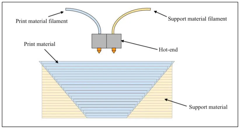
to print support material separately from the actual print material, as shown in Figure 5.

Figure 5: Dual-nozzle extruder. Adapted from Ali, Mir-Nasiri, and Ko 2016

A novel system with five extruders (Ali, Mir-Nasiri, and Ko 2016) aimed to reduce the total print time

by minimizing the time between the first filament’s end of printing and the second filament’s start of

printing in multi-material and multi-color applications. The extruder system has a custom-designed drive

mechanism (rotating probe) capable of holding up to five filaments at any instance, each connected to a

separate nozzle at the hot end. The proposed extruder system has higher efficiency in terms of motor usage,

as it manages the 5-filament system with two stepper motors, as opposed to the standard practice of using

a stepper motor for each filament. One stepper motor is used to select the filament, while the other stepper

only one filament is driven and utilized at a time for printing. Thus, this approach reduces the filament

change time, however, it has no impact on the time taken by printing moves.

A multi-nozzle deposition system for tissue engineering applications (Khalil, Nam, and Sun 2005) uses

four different types of nozzle to deposit materials with different viscosities. The types of nozzles used are

pneumatic micro-valve, piezo-electric nozzle, solenoid micro-valve and precision extrusion deposition

nozzle (PED). A pneumatically operated material delivery system supplies the materials to the nozzles

which actuate based on their adjusted operating pressure. The system can work in droplet mode or extrusion

mode and is capable of heterogeneous deposition, i.e. simultaneous deposition using multiple nozzles for

depositing multiple materials.

Project Escher (Miller 2016) designed by Autodesk is another attempt at reducing the print time by

utilizing multiple nozzles simultaneously. The multiple print heads are mounted on independent gantries,

thus enabling relative motion between them. The project is a software control technology which distributes

the toolpath for a part to be printed amongst the multiple independent print heads to control their deposition

motion while preventing collisions between the heads. The process is well suited for manufacturing parts

with large footprints in the X-Y plane, however, the advantages of the system may be limited for smaller

parts.

2.3.

The techniques discussed earlier in this chapter attempt to minimize the total print time of a part by

optimizing the layer thickness based on the geometry of the part. The dynamic adaptive slicing techniques

further aim to reduce the print time by using maximum layer thickness for the interior of a part and

adaptively slicing only the exterior to achieve the desired surface finish.

The study of the multi-extruder systems also shows multi-color and multi-material printing to be the

This thesis explores the potential of reducing the total print time by utilizing multiple nozzles

concurrently to increase the deposition rate in the X-Y plane. However, unlike Project Escher, the multiple

nozzles are mounted on the same print-head with a fixed offset between the nozzles. Thus, there is no

relative motion between the nozzles. Concurrent printing utilizing this arrangement will help minimize the

limitation of the concurrent systems on the part size. Such multi-nozzle extruders may be utilized

concurrently to print each layer faster, therefore printing the entire part faster as compared to a single nozzle

extruder.

2.4.

“Process Planning for Concurrent Multi-Nozzle 3D Printing”

This thesis aims at developing, demonstrating and exploring the potential of a multi-nozzle concurrent

3D printing process to increase the volume deposition rate and to minimize the trade-off between print time

and surface quality of a part.

The working hypothesis is that printing with multiple nozzles simultaneously will reduce the printing time

for each layer and thus the cumulative time for a given part. Since there is no change along Z axis, the

surface quality of the part is expected to remain unchanged as compared to single nozzle printing.

The subsequent chapters will discuss the methodology, preliminary results and the possible future

CHAPTER 3

METHODOLOGY

This chapter describes the approach adopted for developing the multi-nozzle concurrent printing

process. It explains the nozzle configurations considered, the developed algorithm for concurrent printing,

and the software and hardware modifications required to incorporate the algorithm in a 3-Axis Cartesian

3D printer to build a proof-of-concept machine.

3.1. NOZZLE CONFIGURATIONS

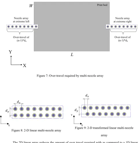
The multiple nozzles in a hot-end can be arranged in a 1D linear array as shown in Figure 6. With this

configuration, however, the over-travel required to allow print bed access to all the nozzles increases as the

number of nozzles increase. Figure 7 shows that the amount of over-travel required by a linear multi-nozzle

array with ‘𝑛’ nozzles can be expressed as ‘2(𝑛 − 1) ∗ 𝑑𝑥’ to access a print bed with length ′𝐿′ and width

′𝑊′, where ′𝑑𝑥′ is the array offset in X direction. To minimize this additional travel movement, nozzles can

instead be arranged in a 2D array. Adjacent rows of nozzles may be perfectly lined up with one other as

shown in Figure 8, or they may be shifted relative to each other as shown in Figure 9. Parameters ′𝑑𝑥′ and

′𝑑𝑦′ represent the array offsets in the X and Y directions respectively.

Figure 6: 1-D linear multi-nozzle array

Figure 7: Over-travel required by multi-nozzle array

Figure 8: 2-D linear multi-nozzle array Figure 9: 2-D transformed linear multi-nozzle array

The 2D linear array reduces the amount of over travel required with as compared to a 1D linear

array with same number of nozzles. However, it introduces a constraint on the possible printing directions,

as the equidistant spacing between the nozzles can be achieved only along specific directions.

Another novel method of compactly arranging multiple nozzles is to use a polygon configuration

where the nozzles are placed at the vertices of the polygon. This thesis considers configurations of regular

′𝑛′ sided polygons with side length of ′𝑠′. Nozzles are numbered in a counter-clockwise direction and are

𝑑

𝑑

𝑑

𝑑

X Y

oriented such that the side connecting the first and the last vertex is parallel to the X axis of the printer as

shown in Figure 10 and Figure 11.

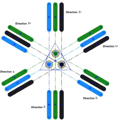
Figure 10: 3-Nozzle polygon array Figure 11: 4-Nozzle polygon array

Similar to the 2D linear configuration, the polygon configuration has constraints on the possible

directions the print head may travel while concurrently printing multiple equally spaced tracks of material.

For an ′𝑛′ sided regular polygon, there are ′𝑛′ axes the print head may travel to produce equidistant tracks

of material. Figure 12 shows the three feasible print axes of motion in the positive and negative directions

for a triangular nozzle configuration. Likewise, Figure 13 shows the four feasible print axes for a square

nozzle configuration.

𝑠

𝑠

X Y

Figure 12: Print directions for a 3-nozzle polygon array

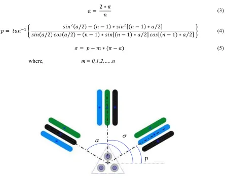
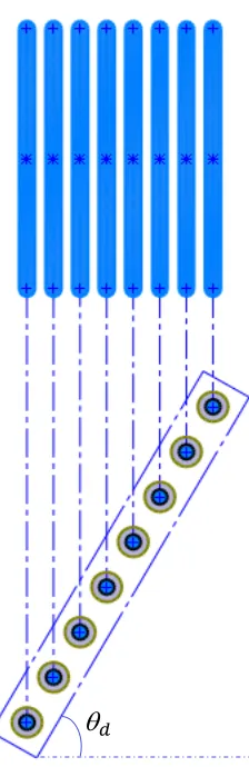
The feasible print orientations for an ′𝑛′ sided polygon nozzle configuration are determined as

follows. The angle ′𝑎′, in radians, is the amount of rotation between each axis of motion. This is obtained

using Equation 3. The angle of the first infill direction relative to the x-axis for an ′𝑛′ sided regular polygon

is given by Equation 4. The angle of the next axis of motion relative to the x-axis is obtained by

incrementing ′𝑝′ by ′(𝜋 − 𝑎)′ radians. This angle ′𝜎′ forms the slope of the infill. Figure 14 shows

utilization of these angles to derive the feasible printing directions.

𝑎 = 2 ∗ 𝜋

𝑛 (3)

𝑝 = 𝑡𝑎𝑛−1{ 𝑠𝑖𝑛

2_{(𝑎/2) − (𝑛 − 1) ∗ 𝑠𝑖𝑛}2_{[(𝑛 − 1) ∗ 𝑎 2⁄ ]}

𝑠𝑖𝑛(𝑎/2) 𝑐𝑜𝑠(𝑎/2) − (𝑛 − 1) ∗ 𝑠𝑖𝑛[(𝑛 − 1) ∗ 𝑎 2⁄ ] 𝑐𝑜𝑠[(𝑛 − 1) ∗ 𝑎 2⁄ ] } (4)

𝜎 = 𝑝 + 𝑚 ∗ (𝜋 − 𝑎)

where, m = 0,1,2,…..n

(5)

Figure 14: Deriving angles for feasible printing directions

The resulting nozzle pitch (i.e. center to center spacing) while printing along these ′𝑛′ directions is given

by Equation 6.

𝑑𝑝=

𝑠

2∗ 𝑐𝑜𝑠 {(𝑎 − 𝜋

2) + 𝑝} (6)

The next sections describe the utilization of these nozzle configurations for concurrent printing.

3.2. ALGORITHM DEVELOPMENT

3.2.1. PRINT HEAD OR PLATFORM ROTATION

3D printed parts are typically printed with a solid skin on top of an interior volume of material that does

not have to be printed fully dense. For example, a solid skin may be printed on top of a hollow honeycomb

structure. Infill density is the 3D printing parameter that allows users to specify this interior volume of

material. Figures 11 and 12 illustrate how multiple tracks of material may be simultaneously printed in

straight lines. The print head nozzle pitch, ′𝑑𝑜′, is fixed when the print head is manufactured and cannot be

dynamically changed during printing. If either the print head or the build platform is able to rotate about a

vertical axis (U-rotation), then it is possible to print equally spaced tracks of material in any direction within

the X-Y plane.

In the case of a 1D linear array of print nozzles, rotational motion allows one to dynamically change

line spacing, as a function of the angle of rotation. This helps achieve the line spacing required to print the

perimeters with two nozzles as well as the line spacing required to achieve the user-specified infill density

when printing with all the nozzles. Figure 15 shows two toolpaths printed using different rotation angles in

order to change the printed line spacing. Adding the ability to rotate either the print head assembly or the

Figure 15: Variable printed line spacing achieved with rotation of a 1D array of nozzles

The rotational angle ′ 𝑑′ required to achieve a desired printed line spacing based on the fixed nozzle

pitch is given by Equation 7.

𝑑 =

𝜋 2− 𝑐𝑜𝑠

−1₍𝑑𝑜

𝑑𝑥

) (7)

When printing outer contours of a given layer using print heads in a polygon configuration with

side length s, the rotational angle ′ 𝑑′ is given by Equation 8.

𝑑 =

𝜋 2− 𝑐𝑜𝑠

−1₍𝑑𝑜

𝑠) (8)

As discussed earlier, when printing the infill with all the nozzles, polygon configuration can print along

a limited number of directions with a resulting printed line spacing of ′𝑑𝑝′. The rotational angle ′ 𝑑′ required

to align nozzles along these directions is given by Equation 9.

𝑑= 𝜎 (9)

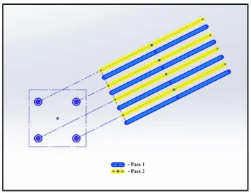
Since the nozzle pitch is fixed at ′𝑑𝑝′ when using a polygon nozzle configuration, multiple passes with

a step-over distance equal to the infill offset ′𝑑𝑜′ are required to achieve the user specified infill density.

Therefore the print head will step-over a distance of ′𝑑𝑜′ for multiple passes based on the ratio of ′𝑑𝑝′ and

′𝑑𝑜′ followed by a step-over distance of ′𝑑𝑝∗ (𝑛 − 1)′. Figure 16 shows polygon configuration using

multiple passes to print infill density smaller than the resulting nozzle offset.

Figure 16: Variable offset achieved with multiple passes for a polygon configuration

In addition to matching the nozzle parameter with infill parameter, the rotational movement is also

is perpendicular to the segment connecting the first and the last nozzle. The rotational angle ′ 𝑣′ at a vertex

′𝑖′ is given below,

𝑣= (𝜋) − [𝑡𝑎𝑛−1(

𝑦𝑖+1− 𝑦𝑖

𝑥𝑖+1− 𝑥𝑖

) − 𝑡𝑎𝑛−1(𝑦𝑖−1− 𝑦𝑖 𝑥𝑖−1− 𝑥𝑖

)] (10)

The rotation is applied to the required coordinates (𝑥, 𝑦) using a transformation matrix to obtain

new coordinates (𝑥𝑇_{, 𝑦}𝑇_{) as shown by Equation 11.}

(𝑥𝑇

𝑦𝑇) = (𝑐𝑜𝑠𝜃_{𝑠𝑖𝑛𝜃} −𝑠𝑖𝑛𝜃_{𝑐𝑜𝑠𝜃} ) (

𝑥

𝑦) (11)

where,

𝜃 = 𝑑 , at the start of print

𝜃 = 𝑣 , at vertex v

The rotational motion serves the purpose of alignment and is therefore an idle movement required at

the start of print to achieve the required offset described earlier and at every vertex for aligning the nozzles

with the next linear segment. This rotational movement can be achieved more conveniently by rotating the

build platform, as opposed to rotating the print-heads, which carry the filaments and the cables to the

hot-ends.

Figure 17: 4-Axis 3D printer

3.2.2. TOOLPATH PLANNING

Utilizing multiple nozzles concurrently requires activating/deactivating individual nozzles at the

endpoints of the respective toolpath segments. This requires defining 2 points for each nozzle for activation

and deactivation, thus requiring a total of ‘2𝑛′ points for ′𝑛′ nozzles. The coordinate system is followed by

the position of the first nozzle and therefore actuation points for all other nozzles are expressed in terms of

the corresponding position of the first nozzle. This is achieved by projecting these actuation points on the

toolpath segments followed by the first nozzle. Thus each toolpath segment assigned to the first nozzle is

divided into ′2𝑛 − 1′ segments by ‘2𝑛’ points to actuate ‘𝑛’ nozzles. The multi-nozzle toolpath currently

supports uni-directional printing.

The toolpath as shown in Figure 18 can be classified into 2 regions, viz. perimeters (or contours)

forming the outer skins and the infill forming the interior region beneath the skin of the part. Toolpaths for

the perimeters and infill are processed separately. Perimeters form one or more closed loops. It is therefore

necessary for the print head to be capable of printing in every direction in order to form a closed loop (i.e.

the contour could be in the form of a circle). Infill patterns, on the other hand, are typically formed by linear

X

Y

raster patterns in one or just a few discrete directions. Perimeters and infill are illustrated in Figure 19 and

Figure 20 respectively.

Figure 18: Toolpath for a layer

Figure 19: Perimeter toolpath for the layer

3.2.2.1.PERIMETERS

Consider the typical case where there are two perimeters for each layer. In this research, the two

perimeters are printed with the first two nozzles when using a 1D linear nozzle configuration and the first

and the last nozzle when using a polygon nozzle configuration.

For each line segment of a given perimeter, it is necessary to define the start and stop points for

each of the two nozzles (i.e. a total of 4 points per printed line segment). As illustrated in Figure 21 below,

one of the two line segments will typically be longer than the other, hence the longer toolpath segment will

be divided into 3 parts. For convex perimeter segments, the outer nozzle path will be longer than the inner

nozzle path. For concave perimeter segments, the inner nozzle path will be longer than the outer nozzle

path. For the sake of discussion, a convex perimeter is assumed. The available coordinates of the outer

toolpath segment are used as actuation points for the first nozzle, and these are used to derive the points for

the other nozzle, viz. second nozzle in case of 1D linear configuration, or the last nozzle in the case of

polygon configurations.

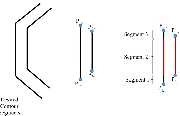
Figure 21: Actuation points for perimeter Desired

Contour Segments

P1,1

P1,2

P2,1

P2,2

P_1,1 P_1,2

P_2,1 P_2,2

This is achieved by defining 4 points relative to each vertex ′𝑖′, as shown in Figure 22. Points 1, 2,

3, and 4 represent the start position of the first nozzle, start position of the second nozzle, projected start

position of the second nozzle on the toolpath segment of the first nozzle when leaving vertex ′𝑖′ and

projected stop position of the second nozzle on the toolpath segment of the first nozzle when approaching

vertex ′𝑖′.

Figure 22: Perimeter toolpath with 2 nozzles

For every vertex ′𝑖′, the coordinates of Point 1 (𝑥1𝑖, 𝑦1𝑖) are available from the 3-Axis g-code file

used as the input for implementing the algorithm, while the coordinates for Point 2 (𝑥2𝑖𝑛, 𝑦2𝑖𝑛), Point 3

Figure 23: 4 points at each vertex

Point 2

𝑥2𝑖 = 𝑥1𝑖+ 𝑠𝑖∗ 𝑐𝑜𝑠 ( 𝑖

2 + 𝛾𝑖) (12)

𝑦2𝑖 = 𝑦1𝑖+ 𝑠𝑖∗ 𝑠𝑖𝑛 ( 𝑖

2 + 𝛾𝑖) (13)

Point 3

𝑥3𝑖 =

𝑚𝑖∗ 𝑦2𝑖 + 𝑥2𝑖 − 𝑚𝑖∗ 𝑐𝑖

𝑚𝑖2 + 1

+ { 𝑑𝑜

𝑡𝑎𝑛 [𝑠𝑖𝑛−1₍𝑑𝑜

𝑑𝑛)]

} ∗ 𝑐𝑜𝑠(𝛾𝑖) (14)

𝑦3𝑖 =

𝑚𝑖2∗ 𝑦2𝑖 + 𝑚𝑖∗ 𝑥2𝑖+ 𝑐𝑖

𝑚𝑖2 + 1

+ { 𝑑𝑜

𝑡𝑎𝑛 [𝑠𝑖𝑛−1₍𝑑𝑜

𝑑𝑛)]

} ∗ 𝑠𝑖𝑛(𝛾𝑖) (15) 𝑖

𝑖

𝑠

𝑑

𝑑

𝑑

(𝑥

, 𝑦

)

(𝑥

, 𝑦

)

(𝑥

, 𝑦

)

(𝑥

, 𝑦

)

Point 4

𝑥4𝑖 =

𝑚𝑖−1∗ 𝑦2𝑖 + 𝑥2𝑖 − 𝑚𝑖−1∗ 𝑐𝑖

𝑚𝑖−12 + 1

+ { 𝑑𝑜

𝑡𝑎𝑛 [𝑠𝑖𝑛−1₍𝑑𝑜

𝑑𝑛)]

} ∗ 𝑐𝑜𝑠(𝛾𝑖−1) (16)

𝑦4𝑖 =

𝑚𝑖−12∗ 𝑦2𝑖 + 𝑚𝑖−1∗ 𝑥2𝑖+ 𝑐𝑖

𝑚𝑖−12 + 1

+ { 𝑑𝑜

𝑡𝑎𝑛 [𝑠𝑖𝑛−1₍𝑑𝑜

𝑑𝑛)]

} ∗ 𝑠𝑖𝑛(𝛾𝑖−1) (17)

where (𝑚𝑖−1, 𝑐𝑖−1) and (𝑚𝑖, 𝑐𝑖) are the slope and the intercept of the toolpath segment approaching

and leaving vertex ′𝑖′ respectively, ′𝑠𝑖′ is a vector drawn from Point 1 to Point 2 at vertex ′𝑖′, and ′𝛾𝑖′ is the

angle made by the segment to be printed between vertices ′𝑖′ and ′𝑖 + 1′ with the horizontal.

𝑠𝑖 = √𝑑𝑜2+ {𝑑𝑜∗ [

1 + 𝑐𝑜𝑠( 𝑖)

𝑠𝑖𝑛( 𝑖)

]}

2

(18)

𝛾𝑖 = 𝑡𝑎𝑛−1(

𝑦𝑖+1 − 𝑦𝑖

𝑥𝑖+1 − 𝑥𝑖

) (19)

The points of interest for actuating the 2 nozzles are Point 1, Point 3 and Point 4 at the current and

destination vertices, as these are the start and stop positions of the nozzles expressed in terms of the location

of the first nozzle.

3.2.2.2.INFILL

While the perimeters are printed with 2 nozzles, the infill is printed with all the ‘𝑛’ nozzles available

with the selected nozzle configuration. We have considered concentric and rectilinear infill patterns for this

thesis.

When using a 1D linear configuration, the actuation points for a concentric infill can be obtained

by generalizing the perimeter algorithm discussed in the earlier section, from 2 nozzles to ′𝑛′ nozzles. These

Point 2 for nozzle ′𝑛′

𝑥2𝑖𝑛= 𝑥1𝑖𝑛+ (𝑛 − 1) ∗ 𝑠𝑖∗ 𝑐𝑜𝑠 ( 𝑖

2 + 𝛾𝑖) (20)

𝑦2𝑖𝑛= 𝑦1𝑖𝑛+ (𝑛 − 1) ∗ 𝑠𝑖∗ 𝑠𝑖𝑛 ( 𝑖

2 + 𝛾𝑖) (21)

As discussed earlier in Section 3.2.1., when using a polygon configuration, the infill points are

processed with multiple print passes separated by a step-over distance of ′𝑑𝑜′. These passes are followed

by a single pass having a step-over distance of ′𝑑𝑝∗ (𝑛 − 1)′. To achieve this, ′𝑑𝑜′ is recalculated such

that it is an integer fraction of ′𝑑𝑝′, and a custom infill is generated. The actuation points for a concentric

infill are obtained using Equations 12 to 19.

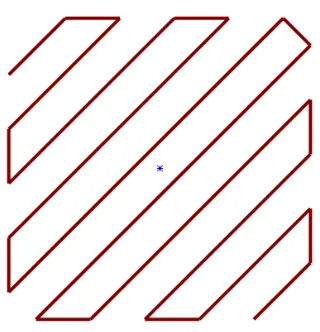
Consider the rectilinear infill shown in Figure 24, where 𝑣0, 𝑣1, 𝑣2 and so on represent the vertices

of the continuous toolpath.

Figure 24: Rectilinear infill

When using a 1D linear configuration for printing a rectilinear infill pattern, nozzle 1 prints the line

segment connecting 𝑣0 and 𝑣1. Nozzle 2 prints the line segment connecting 𝑣2 and 𝑣3, and so on. These

vertices therefore form the end points of the toolpath segments for the corresponding nozzles and are used

connecting 𝑣1 and 𝑣2 is skipped to avoid rotational movement during printing the infill, and the movements

from 𝑣0 to 𝑣1 and from 𝑣2 to 𝑣3 are extended up to the perimeter. In terms of the developed algorithm, the

vertex coordinates form coordinates of Point 1 and Point 2, and the corresponding Point 3 and Point 4

coordinates at each vertex can be obtained using equations 14 through 19.

The user-specified infill angle results in different directions of the infill for alternate layers. These

infill directions are achieved with rotational movement when using a 1D linear configuration of nozzles.

As mentioned earlier, with a polygon configuration of nozzles arranged along an ‘𝑛’ sided regular

polygon, a uniform infill spacing can only be achieved in ′𝑛′ directions separated by angle ′(𝜋 − 𝑎) ′. A

custom infill is generated using the recalculated ′𝑑𝑜′ values such that ′𝑑𝑜′ is an integer fraction of ′𝑑𝑝′.

Some of these ‘𝑛’ directions will have the same orientation with opposing directions (i.e. 0 and 180 degrees,

90 and 270 degrees, etc.) and thus are processed similarly. For instance, when using a 4 nozzle square

hot-end, a uniform infill can be achieved along 4 directions, however, 2 of these printing directions have the

same orientation but with opposing axial directions. Similarly, when using a 3 nozzle triangular

configuration, a uniform infill can be achieved along 6 directions, however 3 of these printing directions

have the same orientation but with opposing axial directions. The sequence of nozzles used in a polygon

configuration also varies with these directions as seen in Figure 12 and Figure 13, as opposed to a linear

array of nozzles where the sequence remains the same.

The required custom infill toolpath is generated using the perimeter toolpath and the slope of

direction of infill. Rays parallel to the direction of infill are created between the extremities of the area

enclosed by the perimeter segments, and intersection points of these rays with all the perimeter segments

are obtained. However, only a few of these points will lie within the region enclosed by the perimeter. These

form the end points of the infill toolpath segments. For instance, when using a polygon configuration for

printing the square shown in Figure 25, the intersection points of a ray with all the 4 perimeter segments

At least 2 points should be obtained for the start and end point of a toolpath, however depending

on the geometry of the part, a toolpath ray may intersect the part multiple times as seen in Figure 26. This

is checked by ensuring that every generated toolpath segment has an even number of intersection points

lying within the area enclosed by the perimeter.

Figure 25: Infill rays intersecting with square

perimeter

Figure 26: Infill rays intersecting with star

perimeter

This generates the vertices of the infill toolpath, which form Point 1 and Point 2 of the developed

algorithm for each nozzle at a vertex. The corresponding Point 3 and Point 4 coordinates at each vertex can

be obtained using Equations 14 through 19. The other directions of infill are used in succeeding layers.

3.2.3. NOZZLE ACTUATION

The points used for nozzle actuation are Point 1 for nozzle 1 and Point 3 for other nozzles at the current

vertex and Point 1 for nozzle 1 and Point 4 for other nozzles at the destination vertex. Figure 27 shows the

the nozzles move from Point 1 at vertex ′𝑖′ to Point 3 at vertex ′𝑖′ to Point 1 at vertex ′𝑖 + 1′ to Point 4 at

vertex ′𝑖 + 1′.

Figure 27: Moving from vertex ‘i’ to vertex ‘i+1’

Appendix I contains the supplemental video demonstrating the motion of the two nozzles along the

actuation points. The actuation state for both the nozzles during these moves is described in Table 1.

Table 1: Nozzle Actuation

Motion from vertex ‘𝒊’ to ‘𝒊 + 𝟏’ First Nozzle Other Nozzle

Rotation by _𝑖

1𝑖 𝑡𝑜 3𝑖

3𝑖 𝑡𝑜 1𝑖+1

1𝑖+1 𝑡𝑜 4𝑖+1

Inactive

Active

Active

Inactive

Inactive

Inactive

Active

Active

1𝑖 3𝑖

The sequence of these moves varies depending on the geometry of the part and size of the part as seen

in Figure 28. The actuation state for the nozzles during these moves is described in Table 2.

Figure 28: Moving from vertex ‘i’ to vertex ‘i+1’ for a smaller part

Table 2: Nozzle actuation for smaller parts

Motion from vertex ‘𝒊’ to ‘𝒊 + 𝟏’ First Nozzle Other Nozzle

Rotation by _𝑖

1𝑖𝑡𝑜1𝑖+1

1𝑖+1𝑡𝑜3𝑖

3𝑖𝑡𝑜4𝑖+1

Inactive

Active

Inactive

Inactive

Inactive

Inactive

Active

Active

To account for this variation, the sequence is determined by sorting the actuation points along the

printing direction. Each of the nozzles is associated with a binary switch in the script which opens a nozzle

once it reaches the start position and keeps it open until the stop position is reached.

3.2.4. RETRACTION

During concurrent printing, multiple nozzles actuate close to the ends of the toolpath segment to

be printed. This may result in oozing of material from the inactive nozzles. As the rotational motion at every

vertex is an idle movement, the nozzles may also ooze during this move. To prevent this oozing, the filament

for a nozzle is immediately retracted when the nozzle is inactivated. It is maintained in a retracted state

until the nozzle is activated for printing again. The retracted amount is fed back in the nozzle before the

printing move. The value of the binary switch is used to determine the required state of the nozzles and to

issue a retracting or unretracting command in the g-code. The resulting process algorithm can be expressed

The following sections describe the implementation of the developed algorithm to build a proof of

concept machine by developing the requisite software and hardware.

3.3. SOFTWARE

3.3.1. G-CODE GENERATION

G-code or ‘Geometric Code’ commands are part of the numerical control programming language used

to provide instructions regarding motion to all the CNC machines including 3D printers. M-code, or

Miscellaneous Code, commands are miscellaneous instructions provided to the machine to set machine

parameters. While each machine may have custom commands defined for specific functions, a few standard

g-code and M-code commands utilized by most 3D printers are listed below in Table 3.

Table 3: Standard g-code commands

Command Description Examples

G# Motion type

G0 – Rapid Linear Move

G1 – Controlled Linear Move

X#, Y#, Z# Coordinates of the destination point X100 Y100 Z8

E# Amount of extrusion

E5 - Extrude 5mm of material (if extrusion

is set to relative)

E5 - Extrude till cumulative value of

extrusion reaches 5mm (if extrusion is set

to absolute)

T# Tool selection T5 – Select tool 5

F# Set the feed rate F1000 – Set feedrate to 1000mm/min

M# Miscellaneous command

A g-code command for a 3-axis 3D printer to travel to 100mm along X and Y axes and 5mm along

Z axis and print 10mm of material at 2000mm/min during the travel would be as follows,

G1 X100 Y100 Z5 E10 F2000;

The algorithm described earlier requires 4 axes to achieve multi-nozzle concurrent printing. Due to the

lack of commercially available 4-axis printers, currently there are no slicers capable of generating 4-axis

g-codes for multiple nozzles. However, there are a plethora of slicers capable of generating 3-axis g-g-codes,

and thus the developed algorithm was implemented in a Perl-based post-processing script template

(Walter), to generate the 4-axis multi-nozzle g-code starting from the 3-axis perimeter and infill toolpaths

generated by these slicers.

The script modifies the 3-axis g-code to add support for:

Rotational axis ‘U’ for the build platform, expressed in degrees;

Activation and/or deactivation of the nozzles at the vertices;

Extrusion values for each extruder which are proportional to the length of the segment to be printed;

Retraction for each nozzle when not printing.

The extrusion values for all the nozzles are associated with ‘E’ command and are separated by a colon. The

syntax for a 3-axis g-code and the post-processed 4 nozzle 4-axis g-code as transformed by the Perl script

is shown below,

G_ X_ Y_ Z_ E_ F_

G_ U_ X_ Y_ Z_ E_:_:_:_ F_

All the coordinates mentioned in the multi-nozzle 4-axis g-code generated by the script are the locations of

the first nozzle in the hot-end configuration, because the algorithm projects the actuation points for all the

other nozzles on the travel segment of the first nozzle as described in Section 3.2.2.

The post-processing script provided in Appendix I requires the 3-axis g-code to:

Be verbose, i.e., have a brief description comment in each line, primarily to distinguish between

Have the extrusion values in relative mode, to determine the proportional extrusion values for each

extruder.

The next section describes the generation of the 3-axis g-code.

3.3.2. SLICER

We have used an open source slicing software called Slic3r (Ranellucci 2011) for generating the

verbose 3-axis g-code from STL files. Slic3r is configured for a given 3D printer. Parameters such as build

plate size, filament size and print temperature allows generation of verbose g-code.

The verbose g-code generated by Slic3r requires the following additions as listed in Table 4, before it

can be processed by the script.

Table 4: Custom g-code additions

Comment Slic3r section

; start of print

T5 ; (Custom tool defined with ′𝑛′ nozzles)

; configuration = (linear/polygon)

; nozzles = (insert number of nozzles)

; vert = (insert number of polygon vertices)

; side = (insert nozzle parameter ′𝑑𝑛′ )

Custom start g-code

; end of print Custom end g-code

A sample verbose 3-axis code program generated by Slic3r and the post-processed 4-nozzle 4-axis

Figure 31: Post-processed 4-nozzle 4-axis g-code

3.3.3. FIRMWARE

The 3D printer built to validate the algorithms developed in this research uses RepRapFirmware to

interpret the multi-nozzle 4-axis g-code generated by the script. The firmware is configured based on the

parameters of the developed printer. These parameters include the end stop types, travel limit locations,

travel speed, and travel acceleration along each axis.

To utilize ′𝑛′ nozzles simultaneously, a new tool T# has to be defined in the firmware to activate all the

3.3.4. G-CODE VISUALISATION

To validate the multi-nozzle 4-axis g-code generated by the post-processing script, a MATLAB-based

simulator, as shown in Figure 32 was developed. Utilizing the multi-nozzle 4-Axis g-code which contains

the coordinates of the first nozzle, the MATLAB script plots the toolpaths for all the nozzles using the

nozzle design parameters ′𝑑𝑛′. The simulator thus helps visualize all the linear and rotational movements

in the 4-axis g-code. It also shows the position of the nozzle array during these movements. A different

color is used for each nozzle to help distinguish the toolpath associated with each nozzle. The simulator

also displays the real-time estimated print time to assist the users. The MATLAB script of the g-code

simulator is provided in Appendix II.

Figure 32: MATLAB g-code simulator

The supplemental videos demonstrating the toolpath simulation for rectilinear and concentric infill with

3.4. HARDWARE

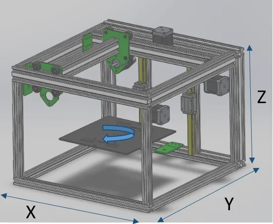
The developed process was demonstrated by building a proof-of-concept 4-axis 3D printer. A 3-axis

custom built Cartesian printer was used as the base system and was modified into a multi-nozzle 4-axis

system for concurrent printing.

The X and Y axes of the base system are driven by a belt system, while the Z axis is driven by a lead

screw system. All axes are driven by NEMA 17 stepper motors. The 3D printer uses a RAMPS 1.4

microcontroller coupled with an LCD display controller with Marlin firmware for interpretation of the

g-code. The mechanical and electronic modifications required to interpret the multi-nozzle 4-axis g-code

generated by the script are mentioned in the following sub-sections.

3.4.1. POSITIONING SYSTEM

The requirement of the rotational axis for the printer was discussed in Section 3.1. The rotational

‘U’ axis is incorporated in the base printer using a rotating build platform. The designed build platform

assembly is shown in Figure 33 and Figure 34.

Figure 34: Build platform assembly (top view, circular build plate set to transparent)

The print bed fixed with a gear on the bottom side, sits on an idle bearing and is connected to the stepper

motor through a pinion. Mounting the build platform on a driven gear, as opposed to being mounted directly

on stepper motor shaft, enables easy disengagement of the build plate for removal of the part. A 200mm

diameter aluminum circular non-heated build plate is used for the developed printer, and the pinion and

gear design parameters are listed in Table 5.

Table 5: Pinion and gear dimensions

Pinion Gear

Teeth 15 70

Diametral pitch 20 in-1 _{20 in}-1

3.4.2. EXTRUDER SYSTEM

As discussed earlier, this thesis utilizes multiple nozzles arranged in a 1D linear configuration and

a polygon configuration for printing concurrently. A commercially available multi-nozzle hot-end (E3D

Kraken) was used to demonstrate both these configurations of the nozzles. Kraken is a 4 nozzle water cooled

hot-end that uses Bowden-style filament feeding. For the linear configuration, 2 rear nozzles 20 mm apart

were utilized. For the polygon configuration, all 4 nozzles arranged along the 20 mm sided square were

used. Figure 35 and Figure 36 show the nozzles used by these configurations looking from the top. Each

nozzle is supplied with an independent 1.75mm filament that is driven by an independent feeder. A separate

stepper motor is therefore required for each of the four nozzles.

Figure 35: 2-nozzle 1-D linear configuration Figure 36: 4-nozzle polygon configuration

The Kraken is attached to the linear bearing of the X-axis carriage using the custom support fixture shown

in Figure 37. The fixture was designed in SolidWorks and 3D printed with a MakerBot Replicator 2X.

𝑑

= 20

𝑠 = 20

Figure 37: Hot-end support fixture: design (left) and with hot-end mounted (right)

As Kraken supports water cooling, the prototype 3D printer utilizes water cooling instead of a fan.

This helps reduce the weight on the X-axis linear carriage, as the requirement for fans and supporting

fixtures will be eliminated from the hot-end support. As Kraken is a Bowden-only extruder, the filament

feeder mechanisms are mounted on the frame of the printer away from the hot-end, thus further reducing

the weight of the moving extruder system mounted on the X-axis bearings. This helps in achieving higher

printing speeds.

3.4.3. CONTROLLER

The developed system uses a total of 8 stepper motors - 4 for the motion axes and 4 for the filament

feeders. Thus, a controller with support for at least 8 stepper motors is required. The RAMPS 1.4 controller

supports a maximum of 5 stepper motors and thus was replaced by a combination of Duet Wi-Fi with Duet

X5 as the expansion board. This setup supports up to 10 stepper drivers. The controller combination uses

RepRap Firmware, which was earlier found suitable for interpretation of multi-nozzle 4-axis g-code.

3.5. PROCESS MAP

Figure 38 shows the process map for the developed concurrent multi-nozzle printing algorithm starting

CAD STL FILE SLICING SOFTWARE 3-AXIS G-CODE

POST-PROCESSING

SCRIPT

4-AXIS G-CODE PRINTING

MATLAB SCRIPT _SIMULATION G-CODE

Figure 38: Process map for the developed multi-nozzle concurrent printing

CHAPTER 4

ANALYSIS & OBSERVATIONS

This section analyzes the developed multi-nozzle concurrent 3D printing process followed by

demonstration of the process capabilities.

4.1. PROCESS ANALYSIS

The developed process utilizes multiple nozzles concurrently, thereby increasing the volume

deposition rate and reducing the print time. However, the new process modifies the commonly used 3-axis

toolpath to introduce the actuation points of multiple nozzles with the corresponding extrusion values and

an additional rotary axis. The resulting 4-axis multi-nozzle toolpath has additional movements as compared

to the 3-axis toolpath. Therefore, the reduction in print time from the process will not be proportional to the

increase in the number of nozzles and has to be studied further.

To understand the relation between the multi-nozzle concurrent printing process and part size for a

given number of nozzles, a parameter ′𝑅𝑖𝑝′ was defined and its print time with multiple nozzles was

analyzed. ′𝑅𝑖𝑝′ is the ratio of the length of infill to the length of perimeter for the toolpath of the part under

consideration.

𝑅𝑖𝑝=

𝑙𝑒𝑛𝑔𝑡ℎ 𝑜𝑓 𝑖𝑛𝑓𝑖𝑙𝑙

𝑙𝑒𝑛𝑔𝑡ℎ 𝑜𝑓 𝑝𝑒𝑟𝑖𝑚𝑒𝑡𝑒𝑟 (22)

To minimize the effect of part geometry on the print time, geometry was limited to square shaped

parts. The parts were designed in SolidWorks and exported as STL files which were then sliced by Slic3r

to generate the 3-axis g-code. The g-code file was post-processed using the script to generate the 4-axis

multi-nozzle g-code file for concurrent printing. Figure 39 shows the CAD model and STL file, while

Figure 39: CAD model (left) and STL file (right) for the 25mm square

Figure 40: 3-axis toolpath (left) and 4-axis 4-nozzle toolpath (right) for 25mm square

The estimated print time was obtained for the first layer from the MATLAB-based g-code simulator script.

Table 6 lists the ′𝑅𝑖𝑝′ values and the estimated print times for printing square parts with multiple nozzles

Table 6: ′𝑅𝑖𝑝′ and estimated print times

Part Size (mm) 𝑹𝒊𝒑 Estimated print times (mins)

2 Nozzles 3 Nozzles 4 Nozzles

25 2.97 1.74 1.77 1.79

50 6.15 4.85 4.44 4.23

100 12.52 15.39 12.65 11.28

150 18.88 31.78 24.75 21.28

200 25.45 53.96 40.76 34.24

4.2. OBSERVATIONS

Figure 41 shows a plot of ′𝑅𝑖𝑝′ for all the part sizes and their corresponding print times as listed in

Table 6.

It can be seen that for lower ′𝑅𝑖𝑝′ values, an increase in the number of nozzles reduces the print time by a

very negligible amount. For higher ′𝑅𝑖𝑝′ values, increasing nozzles helps reduce the print time significantly.

Thus, multi-nozzle concurrent printing process is suitable for parts with larger foot-print in the XY plane.

The process algorithm also results in addition of following movements to the toolpath as compared to a

3-axis toolpath:

rotational movement at every vertex, which is an idle travel move;

printing movement from Point 1 to Point 4 at the destination vertex.

The rotational movement’s frequency and value are a function of the geometry of the part to be printed and

thus has limited scope for minimization. However, the length of the printing movement from

Point

Point

𝑙𝑝=

𝑑𝑜

tan {sin−1₍ 𝑑𝑜

𝑛 ∗ 𝑑𝑥)}

(23)

Thus, it is a function of the number of nozzles, offset between consecutive nozzles ′𝑑𝑥′ and the offset

between the parallel segments ′𝑑𝑜′. The offset between the parallel segments has a positive correlation with

′𝑙𝑝′ and increases with reduction in infill density, which is a parameter specified by the user. The nozzle

offset ′𝑑𝑥′, has a negative correlation with ′𝑙𝑝′ and can be controlled by the user. A more compact

arrangement of nozzles separated by a small offset can yield lower print times for a given part.

The next sub-section demonstrates the process capabilities using the developed proof-of-concept 3D

printer for linear as well as polygon configurations of nozzle arrangements.

4.3. PRINT RESULTS