Origin and dynamical evolution of Neptune Trojans: I. formation and planetary migration

Origin and dynamical evolution of Neptune Trojans – I. Formation

and planetary migration

P. S. Lykawka,

†

J. Horner,

B. W. Jones

and T. Mukai

1_{Department of Earth and Planetary Sciences, Kobe University, 1-1 rokkodai-cho, nada-ku, Kobe 657-8501, Japan} 2_{Department of Physics and Astronomy, The Open University, Walton Hall, Milton Keynes MK7 6AA}

Accepted 2009 June 11. Received 2009 June 10; in original form 2009 February 19

A B S T R A C T

We present the results of detailed dynamical simulations of the effect of the migration of the four giant planets on both the transport of pre-formed Neptune Trojans and the capture of new Trojans from a trans-Neptunian disc. The cloud of pre-formed Trojans consisted of thousands of massless particles placed on dynamically cold orbits around Neptune’s L4 and L5 Lagrange points, while the trans-Neptunian disc contained tens of thousands of such particles spread on dynamically cold orbits between the initial and final locations of Neptune. Through the comparison of the results with the previous work on the known Neptunian Trojans, we find that scenarios involving the slow migration of Neptune over a large distance (50 Myr to migrate from 18.1 au to its current location, using an exponential-folding time ofτ =10 Myr) provide the best match to the properties of the known Trojans. Scenarios with faster migration (5 Myr, withτ =1 Myr), and those in which Neptune migrates from 23.1 au to its current location, fail to adequately reproduce the current-day Trojan population. Scenarios which avoid disruptive perturbation events between Uranus and Neptune fail to yield any significant excitation of pre-formed Trojans (transported with efficiencies between 30 and 98 per cent whilst maintaining the dynamically cold nature of these objects –e <0.1,i <5◦). Conversely, scenarios with periods of strong Uranus–Neptune perturbation lead to the almost complete loss of such pre-formed objects. In these cases, a small fraction (∼0.15 per cent) of these escaped objects are later recaptured as Trojans prior to the end of migration, with a wide range of eccentricities (<0.35) and inclinations (<40◦). In all scenarios (including those with such disruptive interaction between Uranus and Neptune), the capture of objects from the trans-Neptunian disc (through which Neptune migrates) is achieved with efficiencies between∼0.1 and∼1 per cent. The captured Trojans display a wide range of inclinations (<40◦ for slow migration, and<20◦ for rapid migration) and eccentricities (<0.35), and we conclude that, given the vast amount of material which undoubtedly formed beyond the orbit of Neptune, such captured objects may be sufficient to explain the entire Neptune Trojan population.

Key words: methods:N-body simulations – celestial mechanics – Kuiper Belt – minor planets, asteroids – Solar system: formation – Solar system: general.

1 I N T R O D U C T I O N

Objects which orbit the Sun either 60◦ahead or behind a planet in

its orbit are known as ‘Trojans’. These objects, moving within the 1:1 mean-motion resonance (hereafter MMR) of that planet, librate around the locations of its L4 and L5 Lagrange points, and can

_{Present address: International Center for Human Sciences (Planetary} Sci-ences), Kinki University, 3-4-1 Kowakae, Higashiosaka-shi, Osaka-fu, 577-8502, Japan.

†E-mail: [email protected]

Jupiter’s L4 Lagrange point. Since then, over 3000 Jovian Trojans have been discovered, and it is thought that Jupiter’s Trojan clouds may contain more objects than the main asteroid belt. The Jovian Trojans include a number of objects with high inclinations, a fact which current theories of Solar system formation are taking great pains to try to explain (Fleming & Hamilton 2000; Morbidelli et al. 2005).

Jupiter is not the only planet with asteroidal attendants. The Earth is known to have at least three ‘quasi-satellite’ asteroids, while Mars has a retinue of at least four objects (Scholl, Marzari & Tricarico 2005). The discovery of the object 2001 QR322 (Chiang et al. 2003) meant that Neptune became the fourth planet known to be accompanied by a retinue of such objects. Since then, a further five Neptunian Trojans have been discovered, and these bodies may well represent a unique window into the formation of our planetary system, since they are believed to have moved on their current orbits since the planets settled into their current architecture. These Trojans are considered to be primordial objects, rather than temporarily captured bodies (e.g. Horner & Evans 2006), since the best-fitting orbits currently available place them in an area of orbital element phase-space which has been shown to be very highly stable in previous studies on the stability of Neptunian Trojans (Nesvorny & Dones 2002). Since the discovery of these first few objects, conservative unbiased estimates of the population of the Neptunian Trojan family suggest that it houses at least as many large objects as the Jovian family (i.e. objects larger than 50–100 km in diameter), and is likely to be far more populous (containing at least an order of magnitude more objects) (Chiang et al. 2003; Sheppard & Trujillo 2006). Given that it is widely accepted that Jupiter Trojans are at least as numerous as main belt asteroids, the population of Neptune Trojans could easily outnumber that of the main belt.

To some extent, the existence of Neptunian Trojans had long been postulated (e.g. Mikkola & Innanen 1992). However, the high spread of inclinations in the small population discovered to date has caused something of a stir. Under the assumption that Neptune’s Trojans, like Jupiter’s, are primordial objects, stored in the Trojan clouds since the formation of the Solar system, theories which describe the formation of the Solar system must also explain the nature of these objects. Most traditional theories of planetary for-mation involve a fairly gentle and slow accretion of material from a cool, flat disc around the Sun (Pollack et al. 1996; Ida & Lin 2004, and references therein). Such schemes would, as a result of

the dynamically cold disc1 _{from which the objects form, lead one}

to assume that the Neptunian and Jovian Trojan populations should be confined to low inclinations (Marzari & Scholl 1998; Chiang & Lithwick 2005). Fortunately, in the light of these observations and our ever-increasing knowledge of the solar and extra-solar plane-tary systems, recent years have seen the development of a number of more violent variations of cosmogenic theories. These theories, which incorporate the previously established planetary theory of planetary migration (e.g. Goldreich & Tremaine 1980; Fernandez & Ip 1984), and may even invoke the mutual scattering of the giant outer planets, attempt to explain such diverse observations as the presence of hot Jupiters (Butler et al. 1997; Masset & Papaloizou 2003), the proposed Late Heavy Bombardment (Gomes et al. 2005;

1_{In this work, a disc of debris is considered dynamically cold if it has never} experienced significant stirring from external sources, and so mimics the very flat nature of the pre-solar disc. Specifically, we consider discs that contain only objects with eccentricities below∼0.01 and inclinations below ∼0◦.6 to be dynamically cold.

Chapman, Cohen & Grinspoon 2007), the dynamically ‘hot’ popu-lation of Jovian Trojans (Morbidelli et al. 2005), and the structure and dynamics of the Asteroid and Edgeworth–Kuiper belts (Petit, Morbidelli & Chambers 2001; Levison et al. 2008; Lykawka & Mukai 2008).

The unexpected discovery of four high-inclination Neptunian Trojans (objects with inclinations greater than 5◦) leads to the con-clusion that there may be many more highly inclined Trojans than their low-inclination counterparts (Sheppard & Trujillo 2006), given that the discovering surveys were concentrated on the plane of the ecliptic. This proposed excess of highly inclined Neptune Trojans challenges the various mechanisms which have been proposed for the formation of Trojan objects, which invariably only produce Trojans with low orbital inclinations (e.g. Chiang & Lithwick 2005; Hahn & Malhotra 2005). This adds an important new datum to the study of Solar system formation, one which may help to determine which theories are most appropriate for our Solar system (e.g. Ford & Chiang 2007; Lykawka & Mukai 2008; Levison et al. 2008). The Neptune Trojans have also been observed to possess peculiar surface colours, when compared to objects in the various classes of trans-Neptunian objects (Sheppard & Trujillo 2006). This finding adds another constraint which must be explained by future studies of Neptune’s Trojans.

Given these surprising results, it is clearly important to obtain a better understanding of the formation, evolution and dynamical

behaviour of objects in the Neptunian Trojan cloud.2_{All previous}

work carried out to model the behaviour of the Trojans has been based on the existence of an initial population which was present by the time that Neptune had formed. That population was often based, with little stated justification, on an arbitrary eccentricity and inclination distributions, or on the Jovian Trojan population (Gomes 1998; Nesvorny & Dones 2002; Kortenkamp, Malhotra & Michtchenko 2004). However, few studies followed the dynamical evolution of these objects for periods of 1 Gyr or more. Several au-thors investigated the effect of planetary migration resulting from the interaction between the giant planets and the planetesimals re-maining after their formation on the stability of pre-formed Trojans (Gomes 1998; Kortenkamp et al. 2004). Such studies have shown that the survival rate of pre-formed Trojans is typically tens of per cent and is strongly dependent on both the radial extent and the rate of Neptune’s migration through the primordial planetesi-mal disc. Fewer studies have investigated the efficiency with which initially non-resonant objects can be captured to Trojan orbits as a result of planetary migration. Chiang et al. (2003) found that no Trojans were captured from a population of 400 objects, lying initially in a dynamically cold disc at 24.1–29.1 au, as a result of Neptune migrating from 23.1 to 30 au. However, Lykawka & Mukai (2008) reported that a small number of objects could be captured from the trans-Neptunian disc to Trojan orbits, and then survive for long periods, as the disc evolves over a 4 Gyr period.

In this work, we examine both the transport and capture of Trojans as a result of the smooth migration of Neptune over a significant fraction of the outer Solar system, in a manner consistent with many models of planetary formation. We compare the number of objects captured to the Trojan family by the migration of the planet to those that form in situ, and are carried along with it, for cases of both rapid and gentle migration, and for both short (∼7 au) and long (∼12 au) migrations (i.e. for scenarios in which Neptune is initially located

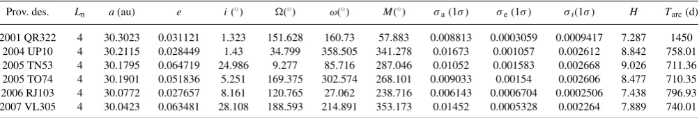
Table 1. List of the currently known Trojans, taken from the Asteroids Dynamic Site – AstDyS4_{. Here,L}

ngives the Neptunian Lagrange point about which the object librates, andHthe absolute magnitude of the object (the apparent magnitude it would have, observed in theVband, if it were placed 1 au from the Earth and the Sun, and displayed a full face to the Earth).Mgives the mean anomaly of the object (2009 Feb. 5),ωgives the argument of the object’s perihelion,ωgives the longitude of its ascending node,igives the inclination of the orbit with respect to the ecliptic plane (all four angles measured in degrees of arc),egives the eccentricity, andagives the semimajor axis (au).σa,e,igives the 1σerror for the variable in question (in the appropriate units), whileTarc gives the orbital arc covered by observations taken into account in the AstDyS orbit computation.

Prov. des. Ln a(au) e i(◦) (◦) ω(◦) M(◦) σa(1σ) σe(1σ) σi(1σ) H Tarc(d)

2001 QR322 4 30.3023 0.031121 1.323 151.628 160.73 57.883 0.008813 0.0003059 0.0009417 7.287 1450 2004 UP10 4 30.2115 0.028449 1.43 34.799 358.505 341.278 0.01673 0.001057 0.002612 8.842 758.01 2005 TN53 4 30.1795 0.064719 24.986 9.277 85.716 287.046 0.01052 0.001583 0.002668 9.026 711.36 2005 TO74 4 30.1901 0.051836 5.251 169.375 302.574 268.101 0.009033 0.00154 0.002606 8.477 710.35 2006 RJ103 4 30.0772 0.027657 8.161 120.765 27.062 238.716 0.006143 0.0006704 0.0002506 7.438 796.93 2007 VL305 4 30.0423 0.063481 28.108 188.593 214.891 353.173 0.01452 0.0005328 0.002264 7.889 740.01

23.1 or 18.1 au from the Sun). This allows us to draw conclusions on the range and rate of Neptunian motion required to excite Trojans to such high inclinations, and to examine which scenario provides the best fit to the currently known Trojan objects.

The model we present represents a significant improvement on the previous work, incorporating a number of new and novel fea-tures. Previous studies have typically considered a single initial

value for Neptune’s heliocentric distance (23 au),3_{although work}

on other aspects of planet formation suggest that it could easily have formed far closer to the Sun. Our work also represents an im-provement of over two orders of magnitude on earlier work in the number of Trojans modelled. Furthermore, we examine how the ef-ficiency with which Trojans are captured during migration depends on the initial orbital eccentricities and inclinations of objects in the trans-Neptunian disc, and carry out the first full study of the dynam-ical evolution of Trojans over the period of Neptunian migration. We consider both captured and pre-formed source populations with initially cold orbital conditions, as would be expected in the early stages of Solar system evolution. We aim to describe the Trojan cloud as a whole, with a particular focus on understanding the ori-gin of the intriguing range of orbital inclinations represented in the known sample of objects. Previous studies were unable to address this point, reporting only individual object captures (e.g. Horner & Evans 2006), or focusing on specific objects, so cannot be consid-ered fully dynamical models of the Trojans (Tsiganis et al. 2005; Li, Zhou & Sun 2007; Lykawka & Mukai 2008).

In Section 2, we will discuss the currently known Trojans, pre-senting the results of simulations intended to identify their stability and general behaviour. In Section 3, we present the method with which runs detailing the capture and transport of Trojan objects as a by-product of Neptunian migration are constructed, before pre-senting a detailed analysis of the results of this work in Section 4. In Section 5, we discuss the implications of our work, and use our results to make predictions about the nature of Neptune’s Trojan clouds, before drawing our conclusions, and discussing fu-ture work, in Section 6.

2 T H E K N OW N N E P T U N I A N T R O J A N S

As of 2009 February 5, six Trojans have been discovered. Their orbital data are displayed in Table 1.4

3_{Hahn & Malhotra (2005) considered Neptune starting at 21.4 au in their} simulations. Gomes (1998) also performed a few simulations with Neptune starting at 21 au.

4_{http://hamilton.dm.unipi.it/}

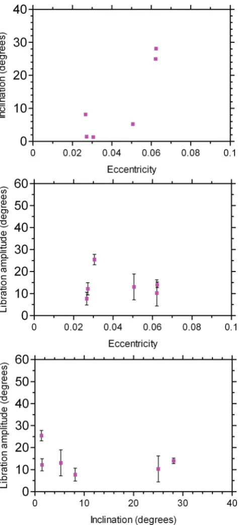
Two things are immediately apparent when one looks at Table 1. First, all of the known Trojans librate around the leading, L4, La-grange point. However, it seems that this result is not actually sta-tistically significant – the surveys which have found these objects have concentrated on the leading Lagrange point, since the trailing, L5, point is currently located around the same area on the sky as the centre of our galaxy (Sheppard & Trujillo 2006). Clearly, when one is searching for faint, slow moving, star-like points, the centre of our galaxy is about the worst possible place to look! Unfortunately, since Neptune is slow moving, it may be a number of years before such observational biases are removed, and a real picture emerges of the degree of symmetry (or indeed asymmetry!) between the pop-ulations around the two Lagrange points. The second detail which is immediately obvious from Table 1 is that the objects seem to be spread in three duplets in inclination. Two objects (2001 QR322 and 2004 UP10) have low inclinations, as would be expected had they formed from a dynamically cold disc. Two Trojans lie at more inter-mediate inclinations (2005 TO74 and 2006 RJ103), while the final two (2005 TN53 and 2007 VL305) are highly inclined to the plane of our system. Even though only these six are currently known, it is obvious that they represent a particularly dynamic and excited population. The orbital properties of the six Trojans are illustrated in Fig. 1.

After the discovery of 2001 QR322, several researchers inves-tigated the orbital properties and stability of this Trojan. Their re-sults indicated that it is likely that 2001 QR322 has been resident within the L4 Trojan cloud for at least 1 Gyr (Chiang et al. 2003; Marzari, Tricarico & Scholl 2003; Brasser et al. 2004). Sheppard & Trujillo (2006) went further, stating that the first four Trojans to be discovered were moving on orbits that are stable over time-scales comparable to the age of the Solar system. More recently, Li et al. (2007) found that 2005 TN53 is also on an apparently highly stable orbit, with stability shown for a 1 Gyr period. Given that, in the current Solar system, Neptune has only an extremely small chance of capturing transient objects as Trojans (Horner & Evans 2006), and taking into account the fact that various studies have shown the currently known objects to be dynamically stable, logic dictates that they are probably primordial bodies (see Dotto et al. 2008 for more details).

Figure 1. General properties of the six currently known Neptunian Trojans. Top: eccentricity versus inclination (◦). Middle: eccentricity versus libra-tion amplitude (◦). Bottom: inclination (◦) versus libration amplitude (◦). The observational data were taken from the AstDyS data base on the 2008 April 24. All six Trojans orbit in the vicinity of Neptune’s L4 point. The libration amplitudes were averaged over individual values calculated for the nominal object plus 100 clones over integrations following their orbits 10 Myr into the future. Here, the libration amplitude refers to the maximum angular displacement from the centre of libration during the object’s reso-nant motion. Libration amplitudes were calculated using theRESTICKcode (Lykawka & Mukai 2007b). The error bars show the statistical errors (at the 1σlevel) resulting from averaging the libration amplitudes over the suite of 101 clones used. Details of the resonant properties of the known Trojans, obtained from these integrations, are shown in Table 2.

Table 2. Resonant properties of the known Trojans, obtained from calculations using RESTICK(Lykawka & Mukai 2007b). The val-ues of mean libration centre (CL, the distance between the mean location of the object and the position of Neptune, in degrees), mean libration amplitude (A, the time-averaged maximum displacement of the object from the centre of libration) and median libration period (TL) are calculated from individual values obtained for the nominal object and 100 clones, after integrating their orbits for 10 Myr. The error bars show the statistical errors (at the 1σlevel) resulting from averag-ing the libration amplitudes over the suite of 101 test particles used.

Prov. des. CL(◦) A(◦) TL(yr)

2001 QR322 66±1 25±2 9200 2004 UP10 61±1 12±3 8850 2005 TN53 59±2 10±6 9450 2005 TO74 61±2 13±6 8850 2006 RJ103 59±1 8±3 8850 2007 VL305 59±1 14±1 9600

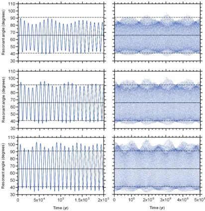
undergoes cycles during which the resonant angle varies from min-imum to maxmin-imum values, as can be seen in Fig. 2. The average

libration amplitude,A, is calculated by sequentially measuring the

individual maximum and minimum displacement values for each clone over the course of the integration, then averaging over these to get the best fit to this value. Effectively, then,Agives the average of the libration amplitudes experienced by all clones of the object over the 10 Myr run.

It is also interesting to calculate the exact location of the centre

of libration (CL) for each object considered, since the libration

followed by a given Trojan is unlikely to be perfectly regular around

the precise location of the L4 point. Typical values forCL will

typically lie within 5◦of the nominal location of the Lagrange point (i.e. 60◦±5◦, 300◦±5◦and 180◦±5◦for L4, L5 and horseshoe orbits, respectively). The libration amplitudes were calculated using theRESTICKcode (Lykawka & Mukai 2007b), with errors calculated

over the dispersion of libration amplitudes obtained for the 101 bodies, and are in agreement with those obtained in previous work (Brasser et al. 2004; Lykawka & Mukai 2007a; Li et al. 2007). As can be seen from Table 2, all currently known Trojans are found to librate with relatively small amplitudes around the L4 point [with the exception of 2001 QR322, whose behaviour we will examine in more detail in a future paper (Horner & Lykawka, in preparation)]. When these results are compared with previous work on the stability of theoretical Trojans (e.g. Holman & Wisdom 1993; Nesvorny & Dones 2002; Marzari et al. 2003; Dvorak et al. 2007), the objects clearly fall in a region that can be considered dynamically stable, supporting the idea that they are primordial objects.

3 M O D E L L I N G P L A N E TA R Y M I G R AT I O N

Figure 2. A small snapshot of the libration behaviour of three clones of 2001 QR322. The behaviour of the clone placed on the nominal orbit of the object is shown in the middle two panels, while the top and bottom panels show the behaviour of the two most extreme clones. Panels on the left-hand side show a short-term snapshot (200 kyr) of the behaviour of the objects, revealing the short-term movement of the clone, in resonant angle (the distance of the object from Neptune, in its orbit, measured in degrees). The right-hand panels show the behaviour over a longer time-scale (5 Myr), with the data plotted as points, allowing the reader to easily see the regions in which the object spends the most time. In each plot, the solid central line marks the location of the centre of libration calculated for the entire sample (CL), while the two dashed lines show the average libration amplitude for the whole sample. It is interesting to note that the clone on the nominal orbit of 2001 QR322 has the great majority of its libration maximum around the location of the average maximum amplitude for the overall sample, while the two extreme examples experience a smaller, or greater, degree of libration.

planets to have undergone significant migration during the later stages of their formation (Fernandez & Ip 1984; Malhotra 1995; Gomes, Morbidelli & Levison 2004; Hahn & Malhotra 2005) – in some cases in a rapid and chaotic manner (e.g. Levison et al. 2008 and references therein). Such migration is considered nec-essary in order to explain a number of the observed properties of our own Solar system (including the structure of the Edgeworth– Kuiper belt and the particular eccentricities and inclinations of ob-jects locked in resonance with Neptune), together with the prop-erties of newly discovered exoplanetary systems (e.g. Masset & Papaloizou 2003).

It is therefore clear that any study of the formation and evolution of the Trojan population must take account of the great changes in the orbital location of the planet during the final years of its

forma-tion. However, to attempt to model each possible variant for Nep-tunian behaviour would be hugely prohibitive, so here we present results on the behaviour of the Trojans in four representative cases.

Two initial starting positions were chosen for Neptune (∼18 and

∼23 au), in an attempt to bracket the minimum and maximum initial

locations suggested for the planet by the past work using the stan-dard models (e.g. Lykawka & Mukai 2008 and references therein). For each of these cases, two scenarios for the migration speed were considered – one in which the planet migrated slowly, taking 50 Myr

to reach its final location at∼30 au (using an exponential-folding

time ofτ=10 Myr), and one with a faster rate of movement (5 Myr

from start to finish, withτ =1 Myr). The integrations were

car-ried out using theN-body packageEVORB(Brunini & Melita 2002),

Table 3. Model parameters. F=Fast migration, S=Slow migration.aU0 andaN0=initial semimajor axis for Uranus and Neptune, respectively.

NdiscandNinsiturefers to the initial number objects used in the disc beyond

Neptune and as pre-formed Trojans. The four principal runs are highlighted in bold text. Single dashes (-) indicate runs in which only pre-formed Trojans were considered, and so no disc objects were present.

Variant code Run aU0(au) aN0(au) τ(Myr) Ndisc Ninsitu

N18-F 1 14.1 18.1 1 30 000 1000

2 14.1 18.1 1 - 1250

3 14.1 18.1 1 - 1668

4 12.6 18.1 1 10 000 1668

N18-S 1 14.6 18.1 10 100 000 60 000

2 14.6 18.1 10 - 1668

3 14.7 18.1 10 - 1668

4 12.2 18.1 10 10 000 1668

N23-F 1 16.1 23.1 1 30 000 1000

2 16.1 23.1 1 - 1668

3 14.8 23.1 1 10 000 1250

4 14.8 23.1 1 - 1668

N23-S 1 16.2 23.1 10 80 000 1000

2 16.2 23.1 10 - 1668

3 14.8 23.1 10 - 1668

4 15.1 23.1 10 - 1668

5 14.8 23.1 10 10 000 1250

semimajor axis would vary according to

ak(t)=ak(F)−δakexp(−t /τ), (1)

whereak(t) is the semimajor axis of the planet after timet,ak(F)

is the final (current) value of the semimajor axis andτis a constant determining the rate of migration of the planet. The fast and slow

migration runs described above employedτvalues of 1 and 10 Myr,

respectively, and the objects were followed for a period of 5τin both cases, after which the planets had reached their current locations. The indexkrefers to the four giant planets, Jupiter (k=J), Saturn (k=S), Uranus (k=U) and Neptune (k=N). Such migration has been modelled in several previous studies (e.g. Malhotra 1995; Chiang et al. 2003; Hahn & Malhotra 2005), and represents a well-accepted simplification for the migration process.

In reality, given that the migration of Neptune would involve it perturbing and displacing a vast number of smaller bodies, initially located in a broad disc beyond the orbit of the planet, varying in size from grains of dust to planetary embryos, the true migration of the planet must have been stochastic and jumpy (Hahn & Malhotra 1999; Murray-Clay & Chiang 2006). This would, in turn, be ex-pected to lower the efficiency with which objects are captured into

the many MMRs migrating ahead of the planet througha-space.

However, given that the mass of Neptune was likely to be far greater than the vast majority of particles it encountered, it is fair to as-sume, as a first approximation, that its migration was reasonably smooth.

Our integrations took into account the gravitational influence of all four giant planets over the course of their migration. Jupiter and Saturn started each run at 5.4 and 8.6 au, respectively. For each Neptunian starting position (18.1 and 23.1 au), additional different initial configurations were tested for Uranus, with the planet starting at locations between 12.2 and 14.7 au (for Neptune starting at 18.1 au), or between 14.8 and 16.6 au (Neptune initially at 23.1 au) (See Table 3). The migration of each planet took place over

identical time-scales (5τ=5 or 50 Myr; dependent on the initialτ

chosen). We set the value ofδakso that the planets migrated from

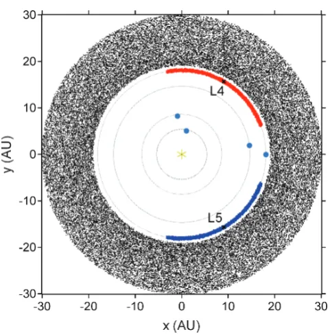
Figure 3. Plot showing the initial locations of all particles used to simulate the evolution of the Trojan population during Neptune’s migration. Though the initial setup for each variant considered would look the same, the particles plotted here are from the scenario which involved Neptune starting at a distance of 18.1 au from the Sun. Objects representing the pre-formed Trojans around the L4 Lagrange point are marked in red, those around the L5 point in blue, while the objects in the trans-Neptunian disc are shown in black. The pre-formed Trojans were placed with an initial displacement of up to 40◦from their Lagrange point, while the disc of objects was distributed on orbits from 1 au beyond the orbit of Neptune to 30 au from the Sun. All particles considered were placed on initially dynamically cold orbits, with e∼i <0.01.

their starting locations to their current ones (in other words, Jupiter migrated inwards, while the other planets migrated outwards).

There are two potential sources for Trojan objects as Neptune marches through the outer Solar system. The first is the population of Trojans expected to form along with the planet, from material located around the two stable Lagrange points within its orbit. As the planet migrates, these objects would be carried along with it, as the 1:1 MMR sweeps outwards. At the same time, it is possible that Neptune would also acquire new Trojans, as objects which grew in the trans-Neptunian region (the aforementioned disc of perturbers) are swept up by the resonance as the planet moves outwards. Thus, the reservoir of objects which formed beyond the planet provides our second source of potential Trojans. Fig. 3 shows a schematic of the initial conditions used for the two distinct populations.

In order to examine the relative contribution of these two popula-tions to the final post-migration Trojan population, clouds of mass-less particles were initially distributed within our simulations over a range of tadpole orbits around both Neptunian Lagrange points, together with a broad disc of objects located beyond the planet.

In the two cases in which Neptune’s migration was fast, 1–3×

104 _{particles were placed in a uniform, dynamically cold, disc}

had to be increased in order to obtain worthwhile statistics. The details of the four cases studied can be seen in Table 3.

The particles in the pre-formed Trojan clouds were smoothly distributed around Neptune’s semimajor axis, with values varying by up to 0.1 au on either side of the planet’s initial location (for the case of N18-S1, where the ease of transport was found to be prohibitively low, the particles were distributed over a larger area, stretching from 17.8 to 18.4 au, and 60 times more test particles were followed, in order to obtain statistically significant results). All pre-formed Trojans had initial eccentricities and inclinations in the range 0–0.01, values typical of a dynamically cold disc (e.g. Hahn & Malhotra 2005 and references therein). Each object was placed

with a random initial libration amplitude,A, such that the objects

lay within±40◦ of either the L4 or L5 point. Finally, the other

rotational orbital elements were randomly determined with values spanning the range 0◦–360◦.

All objects within the disc also started in a dynamically cold, unstirred state, with inclinations below 0.◦6 and eccentricities below

0.01 (∼i). Later, we tested slightly hotter discs (one containing

particles withe <0.05, and a second with particles ofe <0.1, with

inclinations determined frome=sini), in order to check how the

capture efficiency changes as a function of disc excitation. All orbits were integrated over a period of 5τ, after which the giant planets had obtained their present-day orbits after evolving according to equation (1). Bodies that reached heliocentric distances greater than 200 au were removed from the calculation at that point, and not followed any further.

Finally, we used theRESTICKpackage to examine the data, detect

the Trojans present at the end of the simulation and determine their resonant properties.

4 R E S U LT S

By the end of planetary migration, a significant number of objects remained as Trojans, with origins both in the pre-formed clouds and in the trans-Neptunian disc. The full gamut of Trojan behaviour was displayed, with tadpole Trojans around both L4 and L5, and

horseshoe objects. Through the use ofRESTICK, the distribution of

these objects was obtained in both element space (a−e−i) and

resonant properties. In particular, we obtained information for each object on every individual resonance capture event, and results for the integration as a whole. For the individual resonance captures, we calculated the duration of the capture, the type of libration (L4, L5 or horseshoe) and the orbital elements of the object. For the integration as a whole, we obtained the total number of resonant captures, the total time spent in resonance, the number of transitions

Table 5. The results of additional, less detailed data output runs carried out to examine the effect changes to the initial conditions (degree of initial Trojan excitation, initial posi-tions of Uranus and Neptune) had on the results for each variant studied. As with Table 4,Cd details the capture efficiency of particles from the disc of objects spread from just beyond the initial location of Neptune out to 30 au,

Rpgives the fraction of pre-formed Trojans retained at the end of the simulation andNgives the number of Trojans present at the end of the run. Single dashes (-) indicate runs in which only pre-formed Trojans were considered, and so no disc objects were present.

Variant Run Cd(per cent) Rp(per cent) N

N18-F 2 - 38 475

3 - 47 784

4 ∼0.4 98 1635

N18-S 2 - 0 0

3 - <0.1 1

4 ∼0.2 98 1635

N23-F 2 - 87 1451

3 ∼0.3 70 875

4 - 83 1384

N23-S 2 - 33 550

3 - 72 1201

4 - 36 600

5 ∼0 71 888

between different libration styles, the number of periods spent as a horseshoe, L4 or L5 object, and the total time spent in each of these categories.

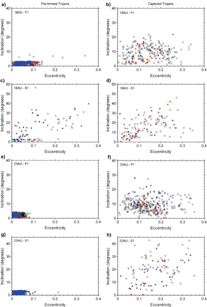
In brief, the Trojans that had been captured from the initially cold disc displayed a wide range of elements, with eccentricities ranging from 0 to 0.35, and inclinations from 0◦to 50◦, while those which had been formed with Neptune and were then transported along with it typically had small eccentricities and inclinations (e <0.1,i <5◦). The one exception to this behaviour was the highly unstable case of slow migration from 18 au (N18-S1-3), which re-sulted in the pre-formed Trojans being excited to orbits ranging up to eccentricities of 0.35 and inclinations of 40◦. In terms of resonant properties, both pre-formed and captured Trojans yielded libration amplitudes from virtually zero (though captured objects rarely at-tained amplitudes less than 10◦) to∼60◦–70◦ for L4/L5 orbits (in the limit of leaving the tadpole orbit) and 150◦–170◦for horseshoe orbits.

As can be seen in Tables 4 and 5, the stability of pre-formed Trojans during planet migration was greatly dependent on both the

Table 4.The statistical results obtained from our principal runs. For each setup, we detail the capture efficiency of Trojans from the trans-Neptunian disc (stretching to 30 au,Cd). In addition,Rpgives the retention fraction of pre-formed Trojans (the fraction of those objects which started the simulations around the L4 and L5 points which are also Trojans at the end of the simulation).NH,NL4andNL5give the number of particles from remaining on horseshoe and tadpole orbits at the end of the simulations (with subscript ‘d’ denoting those captured from the main disc and ‘p’ denoting those which were pre-formed). Finally,fRCgives the ratio of the probability of pre-formed Trojans being retained (Rp) to the likelihood of objects from the disc being captured (Cd).

Variant Run Cd(per cent) NHd NL4d NL5d Rp(per cent) NHp NL4p NL5p fRC

N18-F 1 0.750 174 26 25 54.6 208 141 197 ∼73

N18-S 1 0.120 72 28 20 0.148 37 23 29 ∼1.2

N23-F 1 1.09 268 27 31 96.5 242 352 371 ∼89

initial heliocentric distance and the rate of migration, with survival rates ranging from approximately 98 per cent (18-F4; and 18-S1) to total loss (18-S2 and 18-S3). However, the survival rates for the cases where Neptune started at 23.1 au (several tens of per cent) are in agreement with past work (Gomes 1998; Kortenkamp et al. 2004).

Finally, a relatively large number of Trojans surviving on horse-shoe orbits were obtained in all runs (see Table 4 for details). How-ever, because objects on such orbits are typically unstable, one can expect these objects not to survive over the age of the Solar system, and therefore such objects are not examined in any great detail in this work.

4.1 Behaviour of pre-formed Trojans

An examination of the behaviour of the pre-formed Trojans over the period of Neptune’s migration allows us to determine the effect that the various model parameters considered have on the final distributions of these objects. Tables 4 (which shows the main runs carried out) and 5 (which details subsidiary runs carried out with lower output detail) present the number of objects which survive the duration of Neptune’s migration as Trojan objects, expressed as a percentage of the initial population. For the four main runs, Table 4 also presents the final distribution of the surviving objects among the three categories of Trojan object – L4, L5 and Horseshoe objects.

It is initially clear, from Table 4, that the retention of pre-formed Trojans is greatly dependent on the rate of Neptune’s migration. For both initial values of Neptune’s semimajor axis (18.1 and 23.1 au), we found that far more objects were retained for rapid migration than for slow migration. This initially surprising result may be explained by the fact that a faster migration rate both allows less time for objects to escape from the 1:1 MMR and also means that objects carried within that resonance will spend less time in

de-stabilizing secondary resonances5_{as they sweep through the outer}

Solar system (e.g. See Kortenkamp et al. 2004).

Table 4 also reveals that, for a given migration speed, the shorter the range of Neptune’s migration, the greater the retention of pre-formed Trojans. This result is perhaps less unexpected than the first, since fewer harmful secondary resonances will be encountered before the objects settle in their final locations. Therefore, it is less likely that there will be widespread disruption of the pre-formed Trojan clouds.

More specifically, from Table 4, the scenario which offered the best retention of pre-formed Trojans was that in which Neptune migrated rapidly from 23.1 au. In this case, 96.5 per cent of ob-jects were retained for the course of the planet’s migration. At the other extreme, the scenario with the worst retention rate was that in which Neptune migrated slowly from 18.1 au to its final location. Here, so few objects were retained that the initial population had to be greatly enhanced (to 60 000 objects; see Table 3) in order to obtain reasonable statistics on the nature of surviving objects, with a retention rate of just 0.148 per cent. It is also interesting to note that, in the case of slow migration from 23.1 au, very few objects successfully make the transition between tadpole- and

horseshoe-5_{Secondary resonances often involve commensurabilities between the} char-acteristic libration frequency of objects within a given MMR and other fre-quencies, such as the libration and circulation frequencies of Trojans near that resonance (Murray & Dermott 1999; Kortenkamp et al. 2004).

type orbits, while for the other three scenarios the final number of horseshoe objects is comparable to those on tadpole-type orbits.

Figs 4 and 5 show the distribution of the post-migration Trojan objects for each of the four cases detailed in Table 4, showing the eccentricity and inclination of their orbits (Fig. 4) and their libration angles and inclinations (Fig. 5). A few details are immediately clear from these plots.

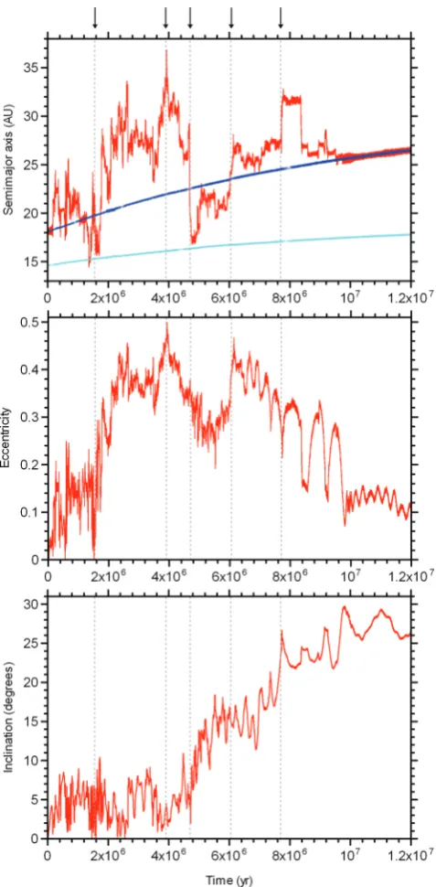
In three out of the four scenarios considered, the initially dy-namically cold swarms of pre-formed Trojans are barely excited in inclination or eccentricity. Even pre-formed Trojans forced on to horseshoe orbits retain their initially low eccentricities and inclinations. In other words, in these scenarios, the pre-formed Trojan clouds are insufficient to explain the observed properties of the modern-day Trojan population. In the case where Neptune migrates slowly outwards from 18.1 au, the pre-formed Trojans are heavily disrupted, being excited to both high inclinations and ec-centricities by severe gravitational perturbations from Uranus and Neptune, leading to an almost complete loss of objects from the pre-formed clouds. However, many of these objects continue to be forced outwards by the planetary migration, and are later recaptured as Trojans, leading to the great similarities which can be seen in the distributions of ‘pre-formed’ and captured populations in that case. Fig. 6 shows a typical example of such behaviour. Note how the particle is initially ejected from the pre-formed cloud, then fol-lows the outward migration of Neptune, hopping between a number of short-lived interior and exterior MMRs, before finally being re-captured as a Trojan. A more detailed explanation of the behaviour of this particular object is given in the caption for Fig. 6.

Slow migration typically leads to fewer tadpole survivors with large libration amplitudes (>60◦) than fast migration. This may, however, be a result of the longer time-scales considered for the slow migration runs – objects with the greatest tadpole libration amplitudes have historically been shown to be the least stable (e.g. Nesvorny & Dones 2002), so this feature may simply be a result of the population of such objects decaying before the end of the run for the slow migration cases. A detailed analysis of the post-migration stability of Trojans obtained in this paper will be given in a future work (Lykawka et al., in preparation).

Figure 6. An example of a pre-formed Trojan being first lost, then recap-tured, from the Trojan cloud during the slow migration of Neptune from 18.1 au. The plots detail the first 12 Myr of the objects evolution, with its semimajor axis, eccentricity and inclination being plotted at top, middle and bottom, respectively. The evolution of Uranus’ and Neptune’s semimajor axes is shown in the upper panel (cyan and blue curves, respectively). The majority of the clone’s evolution is spent drifting within the Trojan cloud, and migrating along with Neptune (this behaviour continues unchanged until the end of the simulations, at 50 Myr;τ=10 Myr). The object experiences a number of close encounters with Uranus and Neptune [marked by sudden large changes in the orbital elements; a few such encounters are marked on the plot (vertical dashed lines)], together with a number of short-term resonant captures (periods of stable, albeit oscillating, orbital elements – e.g. at 7.6 Myr). Finally, the object is recaptured to the Trojan family, albeit with greatly excited inclination.

that the location of Uranus played during the migration of the outer planets, being a major influence on the degree of disruption suffered by the Trojan population (Gomes 1998). A detailed analysis of this phenomenon is beyond the scope of this work, but it will be the subject of a forthcoming paper (Lykawka et al., in preparation).

It should, at this point, be noted that the loss of objects from the pre-formed Trojan cloud was not uniform across those clouds. In-deed, there was a clear link between the initial libration amplitude,A, of the objects and their survival efficiency. Objects with larger initial libration amplitudes were significantly less stable, over the course of planetary migration, than those which experienced smaller-scale libration. As discussed above, this is far from unexpected – the greater the scale of libration, the less stable an object would be expected to be – and so it is natural that the clouds would ef-fectively be whittled away from the outside inwards. However, this

effect was only noticeable for libration amplitudes beyond 30◦–

35◦– the transportation efficiency of objects with smaller libration

amplitudes than this showed little dependence on the initialA.

4.2 Behaviour of captured Trojans

Tables 4 and 5 also detail the efficiency with which the migrating Neptune captured objects from the trans-Neptunian disc. In each of the four main cases (detailed in Table 4), the capture rate observed was actually surprisingly high (between 0.12 and 1.1 per cent), when one considers the amount of scattering that objects in this region must experience as they are stirred by the migrating planet. As for the pre-formed Trojans, the efficiency with which the trans-Neptunian objects were captured is strongly dependent on the speed of the planet’s migration, with cases of fast migration being almost an order of magnitude more efficient in Trojan capture than their slower counterparts. One surprising feature of these capture runs, when compared to the behaviour of pre-formed Trojans (discussed earlier) is that the capture efficiency observed in the run detailing slow migration from 18 au was almost identical to that for the case of slow migration from 23 au. Clearly, the highly destabilizing event which affected the pre-formed cloud of Trojans had little effect on the efficiency with which objects were captured from the trans-Neptunian cloud. This adds further weight to the argument that the destabilization occurred early in the migration of Neptune, and was only effective for a short period – after which the efficiency with which objects were captured from the trans-Neptunian disc was unaffected.

Also obvious from Table 4 is the fact that the captured Trojans move on predominantly horseshoe-type orbits (an eight- to 10-fold excess in the case of fast migration, compared to a two- to three-fold excess for slow migration). Nevertheless, it is interesting to observe that a significant number of objects were captured on to the theoretically more stable tadpole orbits as the result of planetary migration.

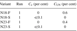
Table 6. The results of additional simulations car-ried out to examine the capture efficiency of Trojans from the extended disc (5000 particles distributed in the range 30–45 au,Ce), and a disc of 5000 ob-jects initially placed between the orbits of Uranus and Neptune (CUN) for our principal runs.

Variant Run Ce(per cent) CUN(per cent)

N18-F 1 0 0.6

N18-S 1 0.1 0

N23-F 1 0 0.4

N23-S 1 0.1 0

the captured Trojans result in fewer objects on low excitation orbits (e <0.05,i <5◦), while there remains an undisrupted relic of the pre-formed Trojan population in that region. From Fig. 5, it is clear that captured Trojans show no real correlation between libration amplitude and orbital inclination, with the interesting result that a number of objects can be captured on to orbits very close to the L4 and L5 point. Presumably, orbits with lower libration amplitudes would be more stable than those with high libration amplitudes, and so such objects could potentially be the source of the known high-inclination Trojans (objects withi >5◦, which all currently

have libration amplitudes less than 15◦– see Tables 1 and 2).

In order to check whether the capture efficiency of trans-Neptunian disc objects to the Trojan clouds was dependent on the initial dynamical state of the disc, two additional small-scale runs were carried out for each of the scenarios in which migration began at 18.1 au. The first such run assumed a slightly ‘hotter’ disc than that used in the key run, with eccentricities up to 0.05 (and using e = sini), and the second assumed a disc that was hotter still, with eccentricities up to 0.1. For both these scenarios, it was found that the capture efficiency was essentially unaltered. The

two additional runs for N18-F yielded Cd values of 0.5 per cent

(e < 0.05) and 0.6 per cent (e < 0.1) (similar to the Cd ∼

0.6 per cent achieved in the main N18-F run), and those for N18-S gaveCdvalues of<0.1 per cent in both cases (again, which is the

same as the∼0.1 per cent obtained in the main N18-S simulation).

Table 5 also details subsidiary runs which examined the effects of different Uranus–Neptune architectures on the efficiency of cap-ture from the trans-Neptunian disc (runs 18F-4, 18S-4, 23F-3 and 23S-2). The small number of captures observed in these runs pre-vent us from drawing too many conclusions on the effect of plan-etary architecture on the capture of trans-Neptunian objects as Trojans during migration, although the initial capture efficiencies seem comparable to those obtained in the key runs.

Finally, Table 6 details the results of additional runs which were carried out to examine the efficiency with which Neptune could capture Trojans from an extended disc (stretching from 30 to 45 au), and the efficiency with which objects were captured from a swarm of objects that were initially distributed between the

or-bits of Uranus and Neptune (acis-Neptunian disc6_{). Each disc was}

populated with 5000 test particles on dynamically cold (e∼i <

0.01) orbits, and was followed until the migration of the planets had stopped. We found that the contribution of bodies from the extended disc to the Trojan cloud was negligible, and so it seems highly un-likely that this region contributed more than a tiny fraction of the

6_{This disc was created so that, at the start of the simulation, its inner edge} was 1 au beyond the orbit of Uranus, and the outer edge was 1 au within the orbit of Neptune.

current Trojan population, unless some event caused it to become significantly excited before the end of planetary migration. In cases

of slow migration, we observed no captures from thecis-Neptunian

disc. However, for cases where the migration was fast, the cap-ture efficiency from this region was found to be approximately 0.5 per cent, comparable to the efficiency with which objects were captured from the Neptunian region. Although the trans-Neptunian disc would span a much greater area of the Solar system, and therefore contain a significantly greater population of objects, it is clear that, at least for rapid planetary migration, the capture of objects which begin on orbits interior to that of Neptune could provide a significant contribution to the final population of captured Trojans.

5 D I S C U S S I O N

In a previous work (Sheppard & Trujillo 2006), the existence of the

high-icomponent of the Trojan population was taken as evidence

that capture mechanisms played a vital role in the creation of the Trojan population. However, our results have shown that, in certain situations, it is feasible that mutual interactions between Uranus and Neptune over the course of their migration can perturb pre-formed Trojans leading to their temporary ejection from the Trojan cloud (Fig. 6). Such objects can then acquire highly inclined and eccentric orbits as a result of successive close encounters with Uranus and Neptune, before being recaptured as Trojans prior to the end of planet migration. This does, however, require the two planets to undergo mutual resonant events (such as the crossing of their mutual 3:4 MMR, or the action of secondary resonances; Kortenkamp et al. 2004). In such cases, the great bulk of pre-formed Trojans would be ejected, with the relic population being almost indistinguishable from that which could be captured as a direct result of Neptune’s migration through a disc of planetesimals. This result reinforces the belief that the mutual locations of Uranus and Neptune can play a pivotal role on the stability of Trojans formed during and after the assembly of both planets.

a result of Neptune’s migration, and will present a detailed analysis of the results in a future work (Lykawka et al., in preparation).

It is clear, therefore, that the existence of a highly inclined component to the Trojan population cannot be used to constrain their source population. Furthermore, since our results suggest that Trojans could arise solely by capture from the disc during a smooth

Neptune migration phase, the known high-iTrojans cannot be used

to directly infer that the planets in the outer Solar system must have experienced turbulent and disruptive resonant events [either resonant interactions and mutual perturbations between Uranus and Neptune (e.g. Gomes 1998; Kortenkamp et al. 2004) or mutual gravitational scattering between these planets (e.g. Levison et al. 2008)].

Given the observed capture efficiencies for objects located on orbits initially beyond the orbit of Neptune, it seems that the most reasonable explanation for the highly excited population of Trojans is simply that it is a direct result of capture during the planet’s mi-gration. Though each of our models is capable of reproducing some aspects of the known Trojans, determining which provides the best fit to the true formation of the Solar system is far more difficult, given the paucity of available observational data. It is worth noting, however, that those simulations which invoked rapid migration of Neptune (runs 18AU-F and 23AU-F) produced few objects with

inclinations greater than 20◦, the majority of which were located

on orbits with relatively large libration, which implies that they would be particularly unstable on Gyr time-scales (Figs 4 and 5). Given that the six known Trojans feature two objects with high in-clinations and comparatively small libration amplitudes (Tables 1 and 2) that appear to be dynamically stable, we suggest that the rapid-migration models face significant problems when attempt-ing to explain the whole observed Trojan population. On the other hand, the results of models featuring more gradual planet migration result in significantly better inclination and libration amplitude dis-tributions, when compared with the observed objects. This suggests that planet migration within the outer Solar system operated at a sedate, rather than hectic, pace. This conclusion is in agreement with the migration time-scales found by Gomes et al. (2004) and Nesvorny, Vokrouhlicky & Morbidelli (2007). Of the two slow mi-gration models considered (18AU-S and 23AU-S), it seems that a more extended migration (18AU-S) is significantly more successful in producing objects with a suitable combination of highly inclined orbits with small libration amplitudes and moderate eccentricities (<0.15), which are like those observed in the known Trojan pop-ulation. However, it is vital that long-term investigations of the resulting Trojan clouds are carried out in order to support the con-clusion that a slow, extended migration of Neptune best explains the observed Trojans, and we are currently in the process of carrying out such work, which will be reported at a later date.

Our examination of the fate of Trojans formedin situhas shown

that, depending on the initial conditions used, they could contribute to the observed Trojan population in one of two ways. In one case, the unusual scenario 18AU-S, pre-formed Trojans are excited (often through a process of ejection and acquisition) to orbits re-sembling those of Trojans captured from the trans-Neptunian disc (i.e.e <0.35,i <60◦). In the other cases, however, where there is a paucity of significant planet-induced instabilities, the pre-formed Trojans result in a dynamically cold (e <0.1,i <5◦) population by the completion of migration. This, therefore, could provide a key observation allowing theorists to determine whether the true migration of Neptune had involved significant interactions with the other planets, or had been more placid in nature. However, it is important to note that the relative importance of the pre-formed

Trojans, when compared to those captured during Neptune’s migra-tion, will be heavily influenced by the size of the initial population of pre-formed Trojans assembled prior to the onset of Neptune’s outward migration. This is still very poorly constrained (Chiang & Lithwick 2005). In particular, although Chiang & Lithwick (2005) showed that accretion was feasible around the leading and trailing Neptunian Lagrange points, the efficiency with which objects can be captured to the Trojan clouds from external reservoirs would appear to suggest that such pre-formed Trojans might be greatly

outnum-bered by their captured brethren.7_{The contribution of pre-formed}

Trojans may also have been negligible if the dynamical conditions around the L4 and L5 points were hostile to accretion (e.g. with objects there excited so that destructive collisions dominated over accretive encounters), preventing the formation of any significant number of objects. Finally, if the migration of the planets led to significantly more disruptive dynamical conditions for the Trojans than those considered in this work (such as could be imagined in scenarios which invoke close encounters between the giant planets themselves), this would clearly cause the loss of most, if not all, of these objects, again rendering their contribution to the final Trojan population negligible.

Our results suggest, therefore, that models of the formation of Neptune’s Trojans can be broken down into two broad scenarios.

(1)Non-chaotic dynamical evolution. Here, as the planets mi-grate to their final locations, Neptune undergoes no significant res-onant interactions with the other outer planets. In such cases, the retention of pre-formed Trojans is significantly more efficient (by two orders of magnitude) than the capture of objects from other reservoirs (Tables 4, 5 and 6). In such scenarios, therefore, in order to explain the observed Trojan distribution (and, in particular, to

avoid creating an excess of low-iobjects when compared with the

observed population), we can conclude that the initial population of pre-formed Trojans must have been significantly smaller than that of objects located in the trans-Neptunian disc of planetesimals. In-deed, from a simple comparison of the volume and surface density of material initially in these regions prior to migration, we would suggest that the amount of mass initially located on pre-formed Trojan orbits would have been at least three orders of magnitude less than that in the disc beyond Neptune (a conclusion in agreement with the accretion model of Chiang & Lithwick (2005).

(2)Chaotic dynamical evolution. In cases where the migration of the giant planets is significantly more chaotic (such as in our key 18AU-S case), the fraction of retained pre-formed Trojans is comparable to the probability that objects will be captured from the trans-Neptunian disc (Table 4). In addition, the resulting distribution

of Trojans ina−e−ispace is such that, with the exception of

a small residue of dynamically cold objects with an origin in the pre-formed clouds, there is little appreciable difference between the different potential formation mechanisms. In such scenarios, we can place no constraints on the relative sizes of the initial populations in the different formation areas.

As we have seen in our results, the effect of such chaotic periods on the transport of pre-formed Trojans can lead to a great variation in both the survival of such objects and the final distribution of

those that remain in the Trojan cloud. If a significant concentration of Trojans is found on dynamically cold orbits, then this would clearly suggest that the migration of Neptune had been unhindered by chaotic interactions between the outer planets, since the only way to produce such a distribution of objects is for that planet to undergo gentle and non-chaotic migration. We found no situation where the capture of objects to the Trojan cloud could produce an excess of such low excitation objects – indeed, if anything, captured objects tend to avoid the region of lowest excitation (e <0.02 and i <4◦). It is the existence of the dynamically cold Trojans, rather than the excited population, that provides the strongest constraint on the formation of the outer Solar system.

To summarize, the observed Trojan population cannot be ex-plained by the presence of pre-formed Trojans alone. Depending on the initial conditions used, it is possible to produce popula-tions of Trojans which mimic that observed today (with some fail-ings which may be explained when the long-term evolution of the Trojans is considered after migration) through either a combination of pre-formed and captured objects, or even by captured objects alone. Unfortunately, the population of known Trojans is currently too small for their orbital distribution to be used to distinguish further between the different scenarios for their formation.

Future observations by missions such asHerschel(Mueller et al.

2009) will carry out the first detailed observational studies of the Neptune Trojan population, allowing better determination of the sizes and physical and chemical compositions. In addition, future very-wide-field survey projects [such as Pan-STARRS (Jewitt 2003) and the LSST (Ivezic et al. 2008)] will lead to at least an order of magnitude improvement in the size of the catalogue of known Trojans, revealing the current orbital structure of the family in more detail. Such work will provide important additional constraints that will help to determine which of the formation scenarios best fit the modern Trojans. Should the Trojans originate from two highly disparate populations, it is likely that this will be reflected in these observations, with the dynamically cold and dynamically hot popu-lations displaying significant differences. Equally, if all (or, at least, the great majority) of the Trojans have origins in the same popu-lation, one would expect observational programmes to reveal the objects to be far more homogeneous in nature. It should be noted that observations of four of the known Trojans suggest they have broadly similar colours, which would suggest that the latter of these scenarios is more likely, although we believe more observations and detailed analysis are necessary in order to draw any firm conclu-sions.

6 C O N C L U S I O N S A N D F U T U R E W O R K

We have carried out the first detailed dynamical simulations of the transport and capture of objects to Neptune’s Trojan population as a function of Neptunian migration. Our results show that both the rate and range of migration can play an important role in determining the survival fraction for pre-formed Trojans, and the capture probability for objects originating elsewhere. In addition, it is clear that the na-ture of the migration (smooth and free from strong perturbations by the other planets versus chaotic and turbulent) can play a significant role in shaping the final distribution of Neptune Trojans. In partic-ular, we found that the transport of pre-formed Trojan populations could be highly disrupted by mutual resonant perturbations between Uranus and Neptune, leading to the almost complete loss of a pre-formed population. However, a small, but significant, fraction of this lost population was eventually re-captured to the 1:1 MMR on orbits stable until the end of migration. Such re-captured orbits exhibited

a much wider range of orbital elements than their brethren that were transported unperturbed, with typical eccentricities as high as 0.35,

and inclinations up to 40◦. Indeed, such recaptured Trojans were

effectively indistinguishable from those captured directly from the trans-Neptunian disc. Conversely, in scenarios which did not result in such perturbations occurring for any prolonged period, we found that pre-formed Trojans were retained with an efficiency between

∼30 and 98 per cent (two orders of magnitude higher than that with

which these objects were captured to the Trojan region from other reservoirs), and remained with dynamically cold orbital conditions, e <0.1,i <5◦.

The efficiency with which objects were captured to the Trojan population, during migration, from the trans-Neptunian disc (which ranged between approximately 0.1 and 1 per cent over the different scenarios) was significantly lower than the retention rate of pre-formed Trojans in the non-disruptive cases. However, this capture rate is sufficiently high that, given that many Earth-masses of mate-rial likely accreted to form planetesimals beyond Neptune’s initial location, the Trojan population could well be dominated by cap-tured objects, even in those cases with the most efficient transport of pre-formed objects. In every scenario considered, the orbits of captured Trojans covered a broad range of eccentricities and incli-nations. Typically, values ranged up to eccentricities of 0.35, and inclinations of 40◦(though we should note that capture during faster migration runs typically led to captured populations with slightly cooler characteristics, with few objects exceeding an inclination of

∼20◦). It is therefore clear that, taking our results as a whole, the highly inclined component of the Neptune Trojan population can be explained reasonably well within the framework of our mod-els. However, of four models considered, we found that the one which best mimicked the observed distribution of Neptune Trojans involved the relatively slow migration of Neptune over an extended distance (from an initial location of 18.1 au). Faster migration, or migration from just 23.1 au, resulted in distributions of objects which failed to reproduce key features of the observed population.

In future work, we will follow the evolution of the Trojan clouds resulting from the various scenarios considered in this work in great detail, examining the behaviour of tens of thousands of objects on a Gyr time-scale in order to better ascertain which scenarios would result in the best fit to the Trojans observed today. We will also examine the effect of a wider range of planetary architectures on pre-formed Trojan clouds.

We believe that future observational campaigns [from missions that will obtain physical and chemical information on the nature

of the Trojans, such as Herschel (Mueller et al. 2009) to those

which will greatly increase the known sample of Trojans, such as Pan-STARRS (Jewitt 2003) and the LSST (Ivezic et al. 2008)] will play a key role in determining which scenarios for planetary migration are a good fit with the observed Trojan population, and encourage observers actively searching for more Trojan objects to avoid limiting their observations to the region close to the ecliptic – the nature and relative population of objects on high-inclination may prove a critical test not only for theories of Trojan formation, but also for models of Neptune’s formation, planetary migration, and the origin and evolution of the outer Solar system.

AC K N OW L E D G M E N T S

Foundation and the Sasakawa Foundation, which proved vital in ar-ranging an extended research visit by JAH to Kobe University. PSL appreciates the support of the COE program and the JSPS Fellow-ship, while JAH appreciates the ongoing support of STFC.

R E F E R E N C E S

Brasser R., Mikkola S., Huang T.-Y., Wiegert P., Innanen K., 2004, MNRAS, 347, 833

Brunini A., Melita M. D., 2002, Icarus, 160, 32

Butler R. P., Marcy G. W., Williams E., Hauser H., Shirts P., 1997, ApJ, 474, L115

Chapman C. R., Cohen B. A., Grinspoon D. H., 2007, Icarus, 189, 233 Chebotarev G. A., 1974, SvA, 17, 677

Chiang E. I., Lithwick Y., 2005, ApJ, 628, 520 Chiang E. I. et al., 2003, AJ, 126, 430

Dotto E., Emery J. P., Barucci M. A., Morbidelli A., Cruikshank D. P., 2008, in Barucci M. A., Boehnhardt H., Cruikshank D. P., Morbidelli A., eds, The Solar System Beyond Neptune. Univ. of Arizona Press, Tucson, p. 383

Dvorak R., Schwarz R., Suli A., Kotoulas T., 2007, MNRAS, 382, 1324 Fernandez J. A., Ip W.-H., 1984, Icarus, 58, 109

Fleming H. J., Hamilton D. P., 2000, Icarus, 148, 479 Ford E. B., Chiang E. I., 2007, ApJ, 661, 602 Goldreich P., Tremaine S., 1980, ApJ, 241, 425 Gomes R. S., 1998, AJ, 116, 2590

Gomes R. S., Morbidelli A., Levison H. F., 2004, Icarus, 170, 492 Gomes R., Levison H. F., Tsiganis K., Morbidelli A., 2005, Nat, 435, 466 Hahn J. M., Malhotra R., 1999, AJ, 117, 3041

Hahn J. M., Malhotra R., 2005, AJ, 130, 2392 Holman M. J., Wisdom J., 1993, AJ, 105, 1987 Horner J. A., Evans N. W., 2006, MNRAS, 367, L20 Ida S., Lin D. N. C., 2004, ApJ, 604, 388

Ivezic Z. et al., 2008, preprint (astro-ph/0805.2366) (http://www.lsst.org/ overview)

Jewitt D. C., 2003, Earth Moon Planets, 92, 465

Kenyon S. J., Bromley B. C., O’Brien D. P., Davis D. R., 2008, in Barucci M. A., Boehnhardt H., Cruikshank D. P., Morbidelli A., eds, The Solar System Beyond Neptune. Univ. of Arizona Press, Tucson, p. 293 Kortenkamp S. J., Malhotra R., Michtchenko T., 2004, Icarus, 167, 347 Levison H. F., Morbidelli A., Vanlaerhoven C., Gomes R., Tsiganis K., 2008,

Icarus, 196, 258

Li J., Zhou L.-Y., Sun Y.-S., 2007, A&A, 464, 775 Lykawka P. S., Mukai T., 2007a, Icarus, 189, 213 Lykawka P. S., Mukai T., 2007b, Icarus, 192, 238 Lykawka P. S., Mukai T., 2008, AJ, 135, 1161 Malhotra R., 1995, AJ, 110, 420

Marzari F., Scholl H., 1998, Icarus, 131, 41

Marzari F., Tricarico P., Scholl H., 2003, A&A, 410, 725 Masset F. S., Papaloizou J. C. B., 2003, ApJ, 588, 494 Mikkola S., Innanen K., 1992, AJ, 104, 1641

Morbidelli A., Levison H. F., Tsiganis K., Gomes R., 2005, Nat, 435, 462 Mueller T. G. et al., 2009, EM&P, 29 (online first)

Murray C. D., Dermott S. F., 1999, Solar System Dynamics. Princeton Univ. Press, Princeton, NJ

Murray-Clay R. A., Chiang E. I., 2006, ApJ, 651, 1194 Nesvorny D., Dones L., 2002, Icarus, 160, 271

Nesvorny D., Vokrouhlicky D., Morbidelli A., 2007, AJ, 133, 1962 Petit J.-M., Morbidelli A., Chambers J., 2001, Icarus, 153, 338

Pollack J. B., Hubickyj O., Bodenheimer P., Lissauer J. J., Podolak M., Greenzweig Y., 1996, Icarus, 124, 62

Scholl H., Marzari F., Tricarico P., 2005, Icarus, 175, 397 Sheppard S. S., Trujillo C. A., 2006, Sci, 313, 511

Tsiganis K., Gomes R., Morbidelli A., Levison H. F., 2005, Nat, 435, 459