Mathematical Model and Parameter Estimation for Tumor Growth

(1)

Rochester Institute of Technology

RIT Scholar Works

Theses

7-25-2018

Mathematical Model and Parameter Estimation for

Tumor Growth

Lujun Yin

[email protected]

Follow this and additional works at:https://scholarworks.rit.edu/theses

Recommended Citation

(2)

Mathematical Model and Parameter Estimation

for Tumor Growth

By

Lujun Yin

A thesis submitted in partial fulfillment of the requirements for the degree of Master of Science

in Applied Mathematics

from the School of Mathematical Sciences Rochester Institute of Technology

25 July 2018

Advisor: Dr. Baasansuren Jadamba Co-advisor: Dr. Akhtar Khan

(3)

Abstract

Numerous models in applied mathematics are expressed as a system of partial differential equations involving certain coefficients. In this work, we consider a tumor growth model originally proposed by Ward and King in 1997. Our main goal is to find an efficient and accurate numerical method for identification of parameters in the model (an inverse problem) from measurements of the evolving tumor over time. The so-called direct problem, in this case, is to solve a system of coupled nonlinear partial differential equations for given fixed values of the unknown parameters. We compare several derivative free and gradient based methods for the solution of the inverse problem which is formulated as an optimization problem with a constraint that is a system of partial differential equations (PDEs). Finally, we modify the original model to include a random parameter and solve the new optimization problem using the Monte Carlo method. The thesis is organized as follows. In the first two intro-ductory chapters, we discuss the original model and the non-dimensionalized version of the model equations. The next chapter is devoted to the optimization formulation of the inverse problem. In the following chapters, we compare performances of the optimization methods. In the final chapter, we discuss the performance comparison of the optimization methods for the cases where the random parameter in the model follows either uniform or truncated normal distributions.

(4)

Dedication

I would like dedicate this to my family, first for their encouragement through the process, and second, for understanding that I would have to give up a lot of time with them in order to pursue my goals.

(5)

Acknowledgement

I would like to thank my family, friends, and mentors for helping me through this learning process, your support was vital to my success.

I am especially grateful for my advisor, Dr. Akhtar Khan and Dr.Baasansuren Jadamba. In the two years I have been their student, he has been patient, kind, and understanding. Dr. Khan and Dr. Jadamba are extremely resourceful and spends much of their valuable time procuring guest speakers and other materials to better aid his students. The multiple viewpoints they provides to each problem is invaluable.

I really love the study experience in RIT. As an international student, I feel different cultures and education there. I am very appreciate to every professor who spent their precious time on teaching me and answering my questions patiently. I will never forget the two years of studying here. I thank everyone in RIT.

Most importantly, I thank my parents for their encouragement for me to complete my degree, they can be most persuasive and motivating. Throughout college, I rarely had the opportunity to visit them for more than a few days at a time, and in a way, they have sacrificed more by having me stay in school. I love my family very much.

(6)

4.2.3 L-BFGS . . . 26

4.2.4 Conjugate Gradient Trust Region Method . . . 27

4.3 Derivative Free Methods . . . 30

4.3.1 Pattern Search Method . . . 30

4.3.2 The Nelder Mead Method . . . 31

4.4 Gradient Projection Method . . . 32

(7)

5.1.1 Pattern Search Method . . . 34

5.1.2 The Nelder Mead Method . . . 38

5.2 Gradient Method . . . 42

5.2.1 Conjugated Gradient Trust Region Method . . . 42

5.2.2 Gradient Projection Method . . . 46

5.3 Analysis . . . 51

6 Tumor growth model with an uncertain parameter 52 6.1 Inverse problem with an uncertain parameter . . . 53

6.2 Numerical solution of the problem . . . 53

6.2.1 Results of the numerical experiments using derivative free methods . . . 54

6.3 Analysis and Future Work . . . 70

(8)

List of Figures

2.1 Microscopic image of neoplastic colonies that grow with an nutrient supply . . . 5

2.2 Direct-fig-radius-1 . . . 9

2.3 Direct-fig-live-cell-density-1 . . . 10

2.4 Direct-fig-concentration-1 . . . 10

2.5 Direct-fig-velocity-1 . . . 11

2.6 Direct-fig-radius-2 . . . 11

2.7 Direct-fig-live-cell-density-2 . . . 12

2.8 Direct-fig-concentration-2 . . . 12

2.9 Direct-fig-velocity-2 . . . 13

5.1 Pattern Search Method Case 1 . . . 35

5.4 The Nelder Mead Method Case 1 . . . 39

5.7 Conjugated Gradient Trust Region Method Case 1 . . . 43

5.10 Gradient Projection Method Case 1 . . . 47

6.1 Normal distribution Parameter Pattern Search Method Case 1 . . . 55

6.4 Uniform Distribution Parameter Pattern Search Method Case 1 . . . 59

6.7 Normal Distribution Parameter The Nelder Mead Method Case 1 . . . 63

(9)

6.11 Uniform Distribution Parameter The Nelder Mead Method Case 2 . . . 68

(10)

Chapter 1

Introduction

1.1

Partial Differential Equation (PDE)

A partial differential equation (PDE) describes a relation between an unknown function and its partial

derivatives. PDEs exist frequently in most topics of physics and engineering. Moreover, in recent

years we have seen a dramatic increase in the applications of PDEs in many areas such as

biol-ogy, chemistry, computer sciences and in economics. The general form of a PDE for a function

u(x₁,x₂, ...,x_n)is

F(x₁,x₂, ...,x_n,u,u_x₁,u_x₂, ...,u_x_n, ...) =0

wherex₁,x₂, ...,x_n are the independent variables,uis the unknown function, andu_x_i denotes the par-tial derivative ∂u

∂xi. The equation is, in general, supplemented by additional conditions such as initial conditions (as we have often seen in the theory of ordinary differential equations (ODEs)) or

bound-ary conditions.

The fundamental theoretical question is whether the problem consisting of the equation and its

asso-ciated side conditions is well-posed. The French mathematician Jacques Hadamard (1865−1963)

coined the notion of well-posedness. According to his definition, a problem is called well-posed if it

(11)

Existence The problem has a solution.

Uniqueness There is no more than one solution.

Stability A small change in the equation or in the side conditions gives rise to a small change in the solution.

If one or more of the conditions above does not hold, we say that the problem is ill-posed. One

can fairly say that the fundamental problems of mathematical physics are all well-posed. However,

in certain engineering applications we might tackle problems that are ill-posed. In practice, such

problems are unsolvable. Therefore, when we face an ill-posed problem, the first step should be to

modify it appropriately in order to render it well-posed.

1.2

Optimization

Optimization is an important tool in decision science and in the analysis of physical systems. To use

it, we must first identify some objective, a quantitative measure of the performance of the system

under study. This objective could be profit, time, potential energy or any quantity or combination of

quantities that can be represented by a single number. The objective depends on certain characteristics

of the system, called variable or unknowns. Our goal is to find values of the variables that optimize

the objective.

The process of identifying objective, variables and constraints for a given problem is known as

mod-eling. Construction of an appropriate model is the first step but the most important step is the

opti-mization step. Once the model has been formulated, an optiopti-mization algorithm can be used to find

its solution. Usually, the algorithm and model are complicated enough that a computer is needed to

implement this process. After an optimization algorithm has been applied to the model, we must be

able to recognize whether it has succeeded in its task of finding a solution. In many cases, there are

elegant mathematical expressions known as optimality conditions for checking that the current set of

(12)

may give useful information on how the current estimate of the solution can be improved. Finally,

the model may be improved by applying techniques such as sensitivity analysis, which reveals the

sensitivity of the solution to changes in the model and data.

1.3

Mathematical Formulation

Mathematically speaking, optimization is the minimization or maximization of a function subject to

constraints on its variables. We use the following notation:

• xis the vector of variables, also called unknowns or parameters;

• f is the objective function, a function ofxthat we want to maximum or minimize;

• c is the vector of constraints that the unknowns must satisfy. This is a vector function of the

variables ofx. The number of components incis the number of individual restrictions that we

place on the variables.

The optimization problem can then be written as

min

x∈Rnf(x) subject to 





c_i(x) =0 i∈ε

c_i(x)≥0 i∈I

(1.1)

(13)

Chapter 2

A Tumor growth model

In this chapter, we include an introduction to a tumor growth model originally introduced by Ward

and King [19] and later considered by D.A.Knopoff [1] and specify the direct and inverse problems

associated to the model.

2.1

The Direct Problem

Scientists believe that mathematical modeling of tumor growth is an effective and important part in

promoting knowledge about cancer, which has become one of the most popular studied topics in

mathematical biology. In the history of mathematical biology,there are many mathematical models of

tumor growth including continuous models and discrete models.

The advantages of continuous models are that they are understandable, tractable to mathematical

anal-ysis and intuitive from biological principles. They contain a few parameters and can use laws from

physics. On the other hand, discrete models are able to work in other scales and each cell can be

treated independently with no extra complication.

Mathematical models of avascular multicellular spheroids are typically continuous models which

con-sist of an ordinary differential equation (ODE) representing the evolution of the outer tumor boundary,

(14)

general approach of modeling, the key variables are the tumor size, e.g., tumor radius, and the

con-centration. Since the tumor changes in size over time, the domain on which the models are formulated

[image:14.612.115.491.155.403.2]

must be determined as part of the solution process, giving a vast class of moving boundary problems.

Figure 2.1: Microscopic image of neoplastic colonies that grow with an nutrient supply

In this work, we consider the model proposed by Ward and King [19]. The tumor is considered to be

a spheroid consisting of a continuous of living cells, in one of two states: live or dead. The rates of

birth and death depend on the nutrient. It is supposed that those processes generate volume changes,

leading to cell movement described by a velocity field. In this tumor growth model, tumor growth

model has the following characteristics:

• Mass of rapidly proliferating cells are supported by the adequate glucose and oxygen

concen-tration of the surrounding environment.

(15)

1. Nutrients are readily available at the rim.

2. Concentration of nutrients significantly decreases as we move from the rim to the

inner-portions of the tumor.

3. Necrotic core reduces the volume.

• Tumor-angiogenesis factors (TAFs) support tumor growth.

Assuming spherical symmetry, the system of equations to be studied is:

∂ η ∂t +

1 r2

∂ r2vη

∂r = [km(ς,θ)−kd(ς,θ)]η (2.1)

∂ η ∂t +

1 r2

∂ r2vς ∂r =

D r2

∂ ∂r

r2∂ η

∂r

−βkm(ς,θ)η (2.2)

1 r2

∂ r2v

∂r = [V1km(ς,θ)−(V1−VD)kd(ς,θ)]η (2.3)

Where the dependent variables η , ς and ν are the live cell density (cells/unit volume), nutrient

concentration and velocity, respectively.

The functionk_mandk_dare taken to be generalized MichaelisMenten kinetics with exponent 1 so that

we can get the following:

k_m(ς,θ) =A_ςς

c+ς

k_d(ς,θ) =B

1−σ ς

ςd+ς

Initial and boundary conditions:

η(r,0) =η1(r)

∂ ς

∂r(0,t) =0

v(0,t) =0

ς(℘(t),t) =c0

d℘

dt =v(℘(t),t)

wherec0 is the external nutrient concentration.Boundary conditions (2.7) and (2.8) reflect the

(16)

2.2

Nondimensionalization and fixed domain method

Following the formulations used in [2],The mathematical model is rescaled and the domain[0,℘(t)]

of the tumor is transformed onto the interval [0,1]. This is a common approach when dealing with

boundary problems. Hence, we define the following functions

N(y,t) =V_Lη(y℘(t/A),t/A)

C(y,t) = _c1

0ς(y℘(t/A),t/A) V(y,t) =_Ar1

0v(y℘(t/A),t/A) S(t) =_r1

0℘(t/A)

a(c,ϑ) = 1_A[km(c,ϑ)−kd(c,ϑ)]

b(c,ϑ) = 1_A[km(c,ϑ)−(1−δ)kd(c,ϑ)]

k(c,ϑ) =Bkb _m(c,ϑ)

Where r0=

3VL

4π

1/3

is the radius of a single cell,δ = V_VD

L,βb=

r2₀β

VLc0D and ϑ = [A,B,cc,cd,σ] with c_c= ςc

c0,cd=

ςd

c0.

The new system that is to be solved on(y,t)domain[0,1]×[0,T]is as follows:

Nt−NyS

0

Sy+ V

SNy=N(a(C,ϑ)−b(C,ϑ)N), 0<y≤1, t >0

C_yy+2_yC_y=K(C,ϑ)NS2, 0<y≤1, t>0

Vy+2_yV =b(C,ϑ)NS, 0<y≤1, t>0

The initial and boundary conditions are :

N(y,0) =N₁(y) =V_L_η_I(y℘(0),0), 0≤y≤1

S(0) =S₁=℘_r(0)

0

(17)

C(1,t) =1, t>0 S0(t) =V(1,t), t>0

Where N₁(y) =V_Lη1(y℘(0),0) and S1= ℘_r(₀0).This system above will be referred to as the direct

problem.This is the system to be numerically solved repeatedly during the optimization procedure.

2.3

Numerical solution of the direct problem

We apply finite difference method to solve the PDEs system of tumor growth model. FunctionsS(t)

andN(y,t)are found by simple time stepping, for example,

N(y,tn+1) =N(y,t) +τ∗

S0

S −

V

SNy+N[a(C,θ)−b(C,θ)N]

t=tn

(2.4)

whereτ is the time step, andtnandtn+1=tn+τ are two consecutive times. The equation forC(y,t)

is solved by the Newton’s method. For the solution ofV(y,t) we use a backward finite difference

scheme and this leads to a linear system involving entries of V at the grid points. For each time step,

we

1 update S (relabelled asS_new).

2 update N (relabelled asN_new) usingS_new.

3 solve for C (relabelled asCnew) via Newton method usingNnew andSnew.

4 solve for V (relabelled asV_new) usingN_new,S_new andC_new.

The pseudocode to update S, N, and solve for V is as follows: GivenS_I (initial dimensionless radius

of a cell calculated throughr₀), whereq is the number of discretization points on the interval[0,1]

andS_new =S_old+τVq.

(18)

• FindCnew by using Newton’s method

• FindN_new.

• Solve a linear system to obtainVnew.

2.4

Experimental Results

In our numerical experiments, we set our parameters as following:

Cc Cd σ Vl δ c0 s0 _βb

0.1 0.05 0.9 10−9 0.5 1.4×10−3 0.021 0.005 Table 2.1: Parameter table

Next, we plot results of some numerical simulations of the direct problem using the parameters values

[image:18.612.160.435.373.575.2]

in Table 2.1.

Figure 2.2: Evolution of the tumor radius S vs. dimensionless time t. where we used time step

(19)

Figure 2.3: Evolution of the live cell densityN vs. dimensionless radiuss. where we used time step

[image:19.612.164.435.72.273.2]

τ=0.0005 andα =50 grid points on[0,1].

Figure 2.4: Evolution of concentrationC vs. dimensionless radiuss. where we used time step τ =

(20)

Figure 2.5: Evolution of velocityV vs. dimensionless radiuss. where we used time step τ=0.0005

[image:20.612.165.435.71.271.2]

andα=50 grid points on[0,1].

Figure 2.6: Evolution of the tumor radius S vs. dimensionless time t. where we used time step

(21)

Figure 2.7: Evolution of the live cell densityN vs. dimensionless radiuss. where we used time step

[image:21.612.164.434.72.273.2]

τ=0.0005 andα =100 grid points on[0,1].

Figure 2.8: Evolution of concentrationC vs. dimensionless radiuss. where we used time step τ =

(22)

[image:22.612.164.434.70.272.2]

Figure 2.9: Evolution of velocityV vs. dimensionless radiuss. where we used time step τ=0.0005

andα=100 grid points on[0,1].

By observing the figures of dimensionless tumor radius figure 2.2 and 2.6, we can find that a slight

kink as the growth rate decelerates a little before reaching the linear phase. This behavior is because

of the time delay from when celss become quiescent to when they die. The live-cell density figure

2.3 and 2.7 show that the live-cell density is relatively constant in a small region beneath the cell

surface, dropping sharply towards zero deeper into the tumour, reflecting a well-defined viable rim

and a necrotic core. It should be stressed that such regions arise naturally from the model rather than

being assumed a priori. Similar, the nutrient concentration figure 2.4 and 2.8 show that the nutrient

concentration decreases sharply through the viable rim and tends to a constant level in the core due to

the nearly complete necrosis in this region. By observing the figure 2.5 and 2.9 of velocity , we can

get the conclusion that the velocity within the tumour decreases very rapidly from a positive value

towards a negative minimum, before approaching zero in the necrotic core. The region of negative

velocity reflects the fact that volume loss by cell death is greater there than the volume gain through

(23)

Chapter 3

Inverse problem

In this chapter, we first give a very brief introduction to inverse problems and ill-posedness. Then,

we will introduce the parameter identification problem rising from the tumor growth model discussed

in Chapter 2. We will also discuss the objective function for the optimization formulation for the

parameter identification problem.

3.1

Definition Of Inverse Problem

Keller [26] formulated the following very general definition of inverse problems, which is often cited

in the literature: We call two problems inverses of one another if the formulation of each involves all

or part of the solution of the other. Often, for historical reasons, one of the two problems has been

studied extensively for some time, while the other is newer and not so well understood. In such cases,

the former problem is called the direct problem, while the latter is called the inverse problem. In

many cases one of the two problems is not well-posed in the following sense: Definition:(Hadamard)

A problem is called well-posed if

• there exists a solution to the problem (existence)

(24)

• the solution depends continuously on the data (stability)

A problem which is not well-posed is called ill-posed. If one of two problems which are inverse to

each other is ill-posed, we call it the inverse problem and the other one the direct problem. All inverse

problems we will consider in the following are ill-posed.

If the data space is defined as set of solutions to the direct problem, existence of a solution to the

inverse problem is clear. However, a solution may fail to exist if the data are perturbed by noise. This

problem will be addressed below. Uniqueness of a solution to an inverse problem is often not easy

to show. Obviously, it is an important issue. If uniqueness is is not guaranteed by the given data,

then either additional data have to be observed or the set of admissible solutions has to be restricted

using a-priori information on the solution. In other words, a remedy against non-uniqueness can be a

reformulation of the problem.

Among the three Hadamard criteria, a failure to meet the third one is most delicate to deal with. In

this case inevitable measurement and round-off errors can be amplified by an arbitrarily large factor

and make a computed solution completely useless. Until the beginning of the last century it was

generally believed that for natural problems the solution will always depend continuously on the

data. If this was not the case, the mathematical model of the problem was believed to be inadequate.

Therefore, these problems were called ill- or badly posed. Only in the second half of the last century

it was realized that a huge number of problems arising in science and technology are ill-posed in

any reasonable mathematical setting. This initiated a large amount of research in stable and accurate

methods for the numerical solution of ill-posed problems. Today inverse and ill-posed problems are

still an active area of research.

3.2

Formulation Of the Minimization Problem

In this section, we will use an inverse problem technique in order to estimate parameters(some of

them unknown)that determines the behavior of a tumor’s growth. We define the following vectors:

(25)

• p= [cc,cd,σ]T

whereφ represents the solution of the direct problem for each choice of the vector of parameters p.

Let us assume that experimental information is available during the time interval 0≤t≤T.Then, the

general problem we are interested in solving can be formulated as:

Find a vector of parameters pthat generates dataφ = [N,V,C,S]T that is the best match to the

exper-imental information over time 0≤t≤T.

For this purpose, we should construct an objective function which gives us a notion of distance

be-tween the experimental (real) data and the solution of the system of PDEs for each choice of

parame-ters p.

We define the following functional:

J(N,S,p) = µ1

2 Z 1

0

Z T

0

[N(y,t)−N∗(y,t)]2dtdy+µ2

2 Z T

0

[S(t)−S∗(t)]2dt (3.1)

where S(t) is the radius evolution obtained by solving the direct problem for a certain choice of p,

S∗ is the evolution measured experimentally (real data).N(y,t) and N∗(y,t) are the living cell

con-centrations for the direct problem solved with the parameters p and the real data (both of them in

the domain[0,1]×[0,T]). The positive constants µ1 andµ2 are introduced, to take into account the

different order of magnitudes betweenN andS. In this way, these two parameters will give us some

flexibility in order to choose an appropriate functional according to the experimental method used to

obtain the data.

(26)

                      

N_t−N_yS_S0y+V_SN_y−N(a(C,p)−b(C,p)N)

Vy+2_yV−b(C,p)NS

C_yy+2_yC_y−K(C,p)NS2 V(1,·)−S0

V(0,·)

C(1,·)−1 C_y(0,·)

N(0,·)−N1

S(0)−S₁

                       (3.2)

In this way we can rewrite the system of PDEs in the previous section asE(φ,p) =0.

The optimization problem that we consider the form:

minimize J(φ,p) =J(S,N,p)

subject toE(φ,p)

p∈Uad

=0

WhereJ: y×U_ad →Ris the objective function andE :y×U_ad →Zis a state equation , foryandz,

Banach spaces andU_ad is a set of admissible points. We assume the following:

1. U_ad ∈Rmis a nonempty , closed and convex set.

2. J:y×U_ad →RandE :y×U_ad →Z are continuously Frechet-differentiable functions.

3. For eachp∈U_adthere exists an unique corresponding solutionφ(p)∈ysuch thatE(φ(p),p) =

0. Thus there is an unique solution operator p∈U_ad 7→φ(p)∈y.

4. The derivative ∂E

∂ φ (φ(p),p):y→Z is a continuous linear operator and it is continuously

in-vertible for all p∈U_ad.

Under these hypothesesφ(p)is continuously differentiable on p∈Uad by the implicit function

(27)

minimizeJe(p) =J(φ(p),p) subject toE(φ,p)

p∈Uad

=0

whereφ(p)is given as the solution ofE(φ(p),p) =0.

To find a minimum of continuously differentiable function Je, it will be necessary to compute the

(28)

Chapter 4

Optimization Methods

4.1

Gradient Method

Optimization refers to finding the maximum or minimum of a real-valued function, which is called

objective function. Since locating the maximum of a function f(x) is equivalent to locating the

minimum of−f(x), it suffices to consider minimization alone in developing computational methods.

Methods for unconstrained optimization fall into two groups, depending on whether derivatives of

the objective function f(x)are used. If an algebraic function is known for f(x), the derivatives can be easily determined by hand or basic algebraic computation in most cases. Derivative information

should be used if it is possible, but there are many reasons why it might not be available. In particular,

the objective function may be too complicated, too high dimensional, or not known in a form that

may be differentiated.

In optimization problems, gradient method is an important algorithm to solve problems of the form

min

x∈Rn f(x) (4.1)

with the search directions defined by the gradient of the function at the current point. In this chapter

we will introduce some optimization methods based on basic idea of gradient method such as the

(29)

4.1.1

Gradient Descent

Gradient descent in [30] is a first-order iterative optimization algorithm to find the minimum of a

function in a local domain. By using gradient descent, we take steps proportional to the negative of

the gradient of the function at the current point. Since the gradient∇f points in the direction of the

steepest growth f , the opposite direction−∇f is the line of steepest descent. How far should we go

along this direction? Now that we have reduced the problem to minimizing along a line, let one of

the one-dimensional methods decide how far to go. After the new minimum along the line of steepest

descent is located, repeat the process, starting at that point. That is, find the gradient at the new point,

and do a one-dimensional minimization in the new direction.

To explain the idea of gradient descent clearly, I will explain the idea depending on an easy example.

Suppose we’re going down a mountain. Firstly we are going down the mountain in any direction for

a distance. Secondly we calculate the gradient of the current point to get a new better direction which

can lead us to go down the mountain more quickly. Thirdly we are going down the mountain in this

new for a distance. Then we just need to do step 2 and 3 again and again until we arrive at the foot of

the mountain. Note: The foot of the mountain represents that the objective function is nearly zero. In

addition new better directions represents the local best direction to go down the mountain.

Algorithm: Gradient descent

fori=0,1,2, ...Do the following steps: Step 1: v=∇f(xi)

Step 2: Minimize f(x−sv)for scalars=s∗ Step 3: x_i+1=xi−s∗v

end

Convergence of Steepest Descent is slower compared with the Newton Method for a good reason.

Newton’s method is solving an equation and is using the first and second derivatives. Steepest

De-scent is actually minimizing by following the downhill direction and is suing only first derivative

(30)

4.1.2

Conjugate Gradient Method

The conjugate gradient method in [29] is an iterative method for solving a linear system of equations

Ax=b (4.2)

whereAis ann×nmatrix that is symmetric and positive definite. The problem can be stated

equiva-lently as the following minimization problem:

f(x) = 1

2x

T_Ax₋_bT_x _(4.3)

Both problems have the same unique solution. This equivalence will allow us to interpret the

Con-jugate Gradient Method either as an algorithm for solving linear systems or as a technique for

mini-mization of convex quadratic functions. We will note that the gradient of phi equals the residual of

the linear system

∇f(x) =Ax−b

de f

=r(x) (4.4)

One of the remarkable properties of the Conjugate Gradient Method is its ability to generate, a set

of vectors with a property known as conjugacy. A set of nonzero vectors{p0,p1, ...,pl}is said to be

conjugate with respect to the symmetric positive definite matrixAif

pT_i Apj=0,f or all i6= j (4.5)

The key observation is that the residual r=b−Ax of the linear system is−∇f(x),the direction of

Gradient descent of the function f at the pointx. Suppose we have chosen a search direction, denoted

by vectord. To minimize f(x)along that direction is to find theα that the functionh(α) =f(x+αd).

We will set the derivative to zero to find the minimum:

(31)

which implies that:

α = r

T_d

dTAd = rTr

dTAd. (4.7)

We conclude from this calculation that we could alternatively solve for the minimum of a paraboloid

by using the Conjugate Gradient Method, but replacing

r_i=−∇f (4.8)

and

αi=α that minimizes f(xi−1+αdi−1). (4.9)

In fact, in looking at it in this way, notice that we have expressed conjugate gradient completely in

terms of f. We can run the algorithm in this form for general f. Near regions where f has a parabolic

shape, the method will move toward the bottom very quickly.

Algorithm: Conjugate Gradient Method

Let(x₀)be the initial guess and setd₀=r₀=−∇f fori=0,1,2, ...that minimizes f(xi−1+αdi−1)

Step 1: x_i=x_i₋₁+αidi−1

Step 2: ri=−∇f(xi)

Step 3: βi= r_iTri

rT_i₋₁ri−1 Step 4: d_i=r_i+βidi−1

(32)

4.1.3

Nonlinear Conjugate Gradient Method

We have noted that the Conjugate Gradient Method can be viewed as a minimization algorithm for

the convex quadratic function f(x) =1₂xTAx−bTx. Similarly we can adapt the approach to minimize

general convex functions, or even general nonlinear functions f. Since there are so many nonlinear

methods based on Conjugate Gradient Method, we only simply introduce one Nonlinear Conjugate

Gradient Method in [5], which is called The Fletcher-Reeves Method. Fletcher and Reeves showed

that an extension of this kind is possible by making two simple changes in Algorithm of Conjugate

Gradient Method. First, in place of the choice for the step lengthα_k, we need to perform a line search

that identifies an approximate minimum of the nonlinear function f along p_k. Second, the residualr,

which is simply the gradient of f in Algorithm of Conjugate Gradient Method, must be replaced by

the gradient of the nonlinear objective f. These two changes give rise to the following algorithm for

nonlinear optimization.

Algorithm: Fletcher-Reeves Method

Givex₀;

Evaluate f0= f(x0),∇f0=∇f(x0);

Set p₀=−∇f₀,k=0; while∇fk6=0

Step 1: Computeαk and setxk+1=xk+αkpk;

Step 2: Evaluate∇fk+1;

Step 3: βk+1=

∇f_kT₊₁∇fk+1

∇fT k∇fk ;

Step 4: p_k₊₁=−∇f_k₊₁+βk+1pk;

Step 5: k=k+1;

(33)

4.2

Optimization Methods Based on Newton’s Method

In this section, we will introduce some optimization methods based on Newton’s method including

Quasi-Newton method, BFGS and L-BFGS.

4.2.1

Quasi-Newton Method

A standard alternative to Newton method is a class of line search methods where the search direction

is defined by

d(j)=−Cj∇f

x(j)

(4.10)

whereCj is updated in each iteration by a quasi-Newton updating formula in such a way that it has

certain properties of the inverse of the true Hessian.

As long asC_jis symmetric positive definite, we have

d(j)

T

∇f

x(j)

<0, that isd(j) is a desecent

direction. To update this matrix we impose the well known secant equation:

Bj+1

αjd(j)

=∇f

x(j+1)

−∇f

x(j)

(4.11)

If we set

s(j)=x(j+1)−x(j) and y(j)=∇f

x(j+1)

−∇f

x(j)

(4.12)

equation 4.11 becomes

B_j+1s(j)=y(j) (4.13)

or equivalently

C_j₊₁y(j)=s(j) (4.14)

(34)

enough to uniquely determineC_j+1. To do that we further require that

C_j+1=argminC

C−Cj

(4.15)

such thatC_j+1in the sense of some matrix norm, be the closest toCj among all symmetric positive

definite matrices that satisfy the secant equation 4.14.

4.2.2

BFGS

BFGS method in [7] is currently thought as the most effective and the most popular quasi-Newton

update formula. The success of the BFGS algorithm depends on how well the updating formula for

Cj approximates the inverse of the true Hessian at the current iteration. Many previous experiments

have shown that the method has very strong self-correcting properties so that if, at some iterations,

the matrix contains bad curvature information, it often takes only a few updates to correct these

inaccuracies. For this reason, BFGS method generally works very well and once close to a minimizer,

it usually attains superlinear convergence.

The most popular update formula is

CBFGS_j₊₁ =

I−ρjs(j)

y(j)

T

C_j

I−ρjy(j)

s(j)

T

+ρjs(j)

s(j)

T

(4.16)

whereρj=

y(j)

T

s(j)

(35)

Algorithm BFGS

Input: x(0),δ,C0

j=0

while true do

d(j)=−C_j∇f

x(j)

αj=Linesearch

x(j),f

x(j+1)=x(j)+αjd(j)

ComputeC_j₊₁from 4.16 and 4.12

j= j+1 if

∇f

x(j)

≤δ then

stop

end if

end while

Output:x(j),f

x(j)

,∇f

x(j)

4.2.3

L-BFGS

Aiming at dealing with the shortcomings of BFGS that requires a lot of storage space, the basic idea

of L-BFGS in [8] is to only store the information of the past miterations to reduce the demand for

data storage space. A less computationally intensive method whennis large is the Limited Memory

BFGS method(L-BFGS). Instead of updating and storing the entire approximated inverse HessianC_j,

the L-BFGS method never explicitly forms or stores the matrix. The first miterations, L-BFGS and

BFGS generate the same search directions.

It can also be stated that L-BFGS method has the further advantage that it only uses relatively new

information. In BFGS method, the inverse Hessian contains information from all previous iterations.

This may be problematic if the objective function is very different in nature in different regions.

(36)

This is remarkable considering that even when using the same number of function evaluations,

L-BFGS runs significantly faster than full L-BFGS ifnis large.

Algorithm: Direction finding in L-BFGS

q=γj∇f

x(j), withγj=

s(j−1)Ty(j−1) y(j−1)Ty(j−1)

−1

fori= (j−1):(−1):(j−m)do

αi=ρi

s(i)

T

q

q=q−αiy(i)

end for

fori= (j−m): 1 :(j−1)do

β =ρi

y(i)Tr

r=r+s(i)(αi−β)

end for Output:d(j)=−r

4.2.4

Conjugate Gradient Trust Region Method

In this subsection, we will introduce a brief algorithm than combines the trust region paradigm with

the inexact Newton ideas.We solve the scaled trust region problem

min kdk_C≤∆

φ(d) (4.17)

where the quadratic model is

φ(d) =∇f(x)Td+1 2d

T

∇2f(x)d (4.18)

Here the C-norm is

kdk_C=

q

(37)

This is a method in that the approximate solution of the trust region problem lies on a piecewise linear

path with the CG iterations as nodes.[27] As long as CG is performing properly nodes are added to

the path until the path intersects the trust region boundary. If a direction of indefiniteness is found,

then that direction is followed to the boundary. In this way a negative curvature direction, if found in

the course of the CG iteration, can be exploited.

The inputs to Algorithm trcg are the current pointx, the objective f, the forcing term , and the current

trust region radius . The output is the approximate solution of the trust region problem d. This

algorithm is not the whole story, as once the trust region problem is solved approximately, one must

(38)

AlgorithmTrcg(d,x,f,M, , ,K_max)

1.r=−∇f(x),ρ0=krk22,k=1,d=0

2.Do while√ρk−1≥ηk∇f(x)k2andk<kmax

(1)z=Mr

(2)τk−1=zTr

(3) ifk=1 thenβ =0 and p=z

elseβ = τ_τk−1

k−2,p=z+βp (4)ω =∇2f(x)p

if pTω≤0 then

findτ such thatkd+τpk_C=∆ d=d+τp;return

(5)α = τk−1

pT_ω (6)r=r−α ω

(7)ρk=rTr

(8)db=d+αp (9) If db

C>∆then

findτ such thatkd+τpk_C=∆ d=d+τp; return

(10)d=db;k=k+1

(39)

Algorithmcgtrust(x,f,τ)

1.Initialize∆,M,η,kmax

2.Do forever

(1) Letx_c=x. Compute∇f(xc).

(2) UseTrcg(d,x,f,M, , ,K_max)to solve the trust region subproblem. Setx_t=x+d. (3) Solve the trust region subproblem with algorithm trcg

(4) Update

4.3

Derivative Free Methods

4.3.1

Pattern Search Method

Sometimes it is not convenient or not possible to know the first or second derivatives of the objective

function in an unconstrained nonlinear problem. In the case we can use pattern search methods which

need only the ability to return the value of f(x)for some input pointx. For this reason they are also known as derivative-free, direct search or black box optimization methods. Pattern search methods

can also be applied when the objective function is differentiable, but in that case we are ignoring

the useful information about the first and second derivatives. Therefore pattern search methods are

typically applied only when the derivatives are not available.

Many pattern search methods have been developed over the years. Pattern search methods follow

the general form of most optimization methods: given an initial guess at a solutionx0 and an initial

choice of a step length parameter∆0>0. [29]Pattern search methods only require simple, as opposed

(40)

Algorithm General Pattern search method

Fork=0,1, ...

(1) Check for convergence

(2) Compute f(x_k)

(3) Determine a stepS_k using Exploratory moves(∆k,Pk)

(4) If f(x_k)> f(x_k+s_k),thenx_k₊₁=x_k+x_k. Otherwisex_k₊₁=x_k. (5) Update(∆k,Pk)

4.3.2

The Nelder Mead Method

The Nelder Mead simplex algorithm in [9] maintains a simplex S of approximations to an optimal

point. In this algorithm the verticesx_j N+1

j=1 are sorted according to the objective function values

f(x₁)≤ f(x₂)≤ · · · ≤ f(x_N₊₁) (4.20) x₁is called the best vertex andx_N₊₁the worst. If several vertices have the same objective value asx₁, the best vertex is not uniquely defined, but this ambiguity has little effect on the performance of the

algorithm.

The algorithm attempts to replace the worst vertexx_N₊₁with a new point of the form

x(µ) = (1+µ)x−µxN+1 (4.21)

wherexis the centroid of the convex hull of{xi}Ni=1

x= 1

N

∑

i=1

xi (4.22)

(41)

Algorithm nelder. Our formulation of the algorithm allows for termination if either f(x_N+1)f(x1)is

sufficiently small or a user-specified number of function evaluations has been expended.

Algorithm nelder(S,f,τ,kmax)

1. Evaluate f at the vertices ofSand sort the vertices ofS.

2. Set fcount=N+1.

3. While f(x_N₊₁)−f(x₁)>τ

(a) Computex,x(µr)and fr= f(x(τr)). fcount= fcount+1.

(b) Reflect: If f_count=k_max then exit. If f(x₁)≤ f_r≤ f(x_N), replacex_N₊₁withx(τr)and go to step 3(g).

(c) Expand: If fcount=kmax then exit. If fr< f(x1)then compute fe= f(x(τe)). fcount= fcount+1.

If f_e< f_r, replacex_N₊₁withx(τe);

otherwise replacexN+1withx(τr)and go to step 3(g).

(d) Outside Contraction: If f_count =k_maxthen exit. f(x_N)≤ f_r≤ f(x_N₊₁), compute f_c= f(x(τoc)).

fcount= fcount+1.

If f_c≤ f_r replacex_N₊₁withx(τoc)and go to step 3(g); otherwise go to step 3(f).

(e) Inside Contraction: If fcount =kmaxthen exit.If fr ≤ f(xN+1)compute fc= f(x(τic)).

f_count= f_count+1.

If fc≤ f(xN+1), replacexN+1withx(τic)and go to step 3(g); otherwise go to step 3(f).

(f) Shrink: If f_count ≤k_max−N, exit. For 2≤i≤N+1: setx_i=x₁−(x_i−x₁)/2; compute f(x_i). (g) Sort: Sort the vertices ofSso that f(x1)≤ f(x2)≤ · · · ≤ f(xN+1).

4.4

Gradient Projection Method

Gradient project methods [6] are methods for solving bound constrained optimization problems. In

solving bound constrained optimization problems, active set methods face criticism because the

ing set changes slowly; at each iteration, at most one constraint is added to or dropped from the

work-ing set. If there arek0constraints active at the initialW0, butkconstraints active at the solution, then

(42)

large problems if the working set at the starting point is vastly different from the active set at the

solu-tion. As a result, researchers have developed algorithms that allow the working set to undergo radical

changes at each iteration and to interior-point algorithms that do not explicitly maintain a working

set.

The gradient-projection algorithm is the prototypical method that allows large changes in the working

set at each iteration. Givenx_k, this algorithm searches along the piecewise linear path

P[x_k−α∇f(xk)],α ≥0 (4.23)

wherePis the projection onto the feasible set. A new point

x_k+1=P[xk−αk∇f(xk)] (4.24)

is obtained when a suitable k>0 is found. For bound-constrained problems, the projection can be

easily computed by setting

[P(x)]_i=mid{x_i,l_i,u_i} (4.25)

where mid{·}is the middle (median) element of a set. The search forkhas to be done carefully since

the function

φ(α) = f(P[xk−αk∇f(xk)]) (4.26)

If properly implemented, the gradient-projection method is guaranteed to identify the active set at a

solution in a finite number of iterations. After it has identified the correct active set, the

gradient-projection algorithm reduces to the steepest-descent algorithm on the subspace of free variables. As

a result, this method is invariably used in conjunction with other methods with faster rates of

(43)

Chapter 5

Numerical Results

In this chapter, we will apply different optimization methods to solve the inverse problem associated to

the tumor growth model including derivative free methods and gradient based methods. We compare

the accuracy and efficiency of the optimization methods.

5.1

Derivative Free Methods

In this section, we apply pattern search method and the NelderMead method to get the solution of the

inverse problem of the tumor growth model including the estimatedN,Sand estimated parameters(C_c,C_d,σ).

5.1.1

We present the results of some numerical simulations using pattern search method in this subsection.

In Figures 5.4, 5.5, 5.6 we present results of three simulations with 1%, 5%, and 10% noise levels.

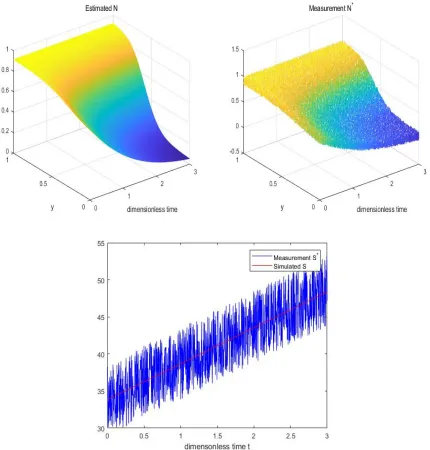
Top left image corresponds to the simulated N (obtained by solving the direct problem by using the

identified values of the parameters). Top right image shows the noisy data fed to the optimization

routine. Bottom row image shows data S∗ (with added noise) and the simulated S. Pattern search

(44)

[image:44.612.89.521.62.513.2]

(45)

[image:45.612.89.521.63.514.2]

(46)

[image:46.612.90.520.63.513.2]

(47)

Noise Level Estimated parameters Relative error CPU time 1% (0.0991,0.0491,0.8985) (0.88%,1.67%,0.15%) 2292.28s 5% (0.1028,0.0518,0.9001) (2.80%,3.60%,0.01%) 2370.48s 10% (0.0948,0.04483,0.8939) (5.18%,10.32%,0.67%) 2293.10s Table 5.1: Exact parameters=(0.1,0.05,0.9), grid points=40, time step=0.005

Noise Level Estimated parameters Relative error CPU time

1% (0.1000,0.0500,0.9005) (0.01%,0.18%,0.06%) 8326.84s 5% (0.0957,0.0451,0.8880) (4.22%,9.78%,1.32%) 8014.07s 10% (0.1050,0.0544,0.9053) (5.09%,8.81%,0.59%) 9116.46s Table 5.2: Exact parameters=(0.1,0.05,0.9), grid points=80, time step=0.0025

Tables 5.1 and 5.2 show the summaries of two sets of simulations with varying number of

discretiza-tion points in the mesh (and time steps).Pattern search method is very effective for our problem. As

the tables show that the method is quite robust with respect to relatively high noise level of 10%.

Simulation times are quite reasonable for a derivative-free method, and they stay roughly the same

during the simulations with varying levels of noise.

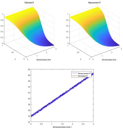
5.1.2

The Nelder Mead Method

We present the results of some numerical simulations using Nelder-Mead method in this subsection.

In Figures 5.4, 5.5, 5.6 we present results of three simulations with 1%, 5%, and 10% noise levels.

(48)

[image:48.612.89.521.62.513.2]

(49)

[image:49.612.89.521.63.515.2]

(50)

[image:50.612.89.520.63.512.2]

(51)

discretiza-tion points in the mesh (and time steps).The Nelder Mead Method is more effective for our problem.

As the tables show that the method is quite robust with respect to relatively high noise level of 10%.

Simulation times are quite reasonable for a derivative-free method, and they stay roughly the same

during the simulations with varying levels of noise. Comparing with Pattern Search Method, Nelder

Mead Method works better for our problem between two derivative free methods.

5.2

Gradient Method

In this section, we apply Conjugated gradient trust region method and Gradient projection method to

get the solution of the inverse problem of the tumor growth model including the estimated N,Sand

estimated parameters(C_c,C_d,σ).

5.2.1

Conjugated Gradient Trust Region Method

We present the results of some numerical simulations using Conjugated Gradient Trust Region Method

(52)

lem by using the identified values of the parameters). Top right image shows the noisy data fed to the

[image:52.612.90.519.115.569.2]

optimization routine. Bottom row image shows dataS∗(with added noise) and the simulatedS.

(53)

[image:53.612.90.520.63.516.2]

(54)

[image:54.612.90.521.64.513.2]

(55)

Noise Level Estimated parameters Relative error CPU time 1% (0.1001,0.0502,0.9004) (0.15%,0.46%,0.04%) 380.00s 5% (0.0984,0.0487,0.8978) (1.55%,2.48%,0.24%) 297.68s 10% (0.1120,0.0626,0.9220) (12.07%,25.23%,2.45%) 334.48s Table 5.5: Exact parameters=(0.1,0.05,0.9),grid points=40,time step=0.005

1% (0.1000,0.0501,0.9007) (0.01%,0.37%,0.08%) 543.00s 5% (0.0965,0.0468,0.8947) (3.48%,6.24%,0.58%) 1214.29s 10% (0.0958,0.0427,0.8801) (4.11%,14.53%,2.20%) 1404.43s Table 5.6: Exact parameters=(0.1,0.05,0.9),grid points=80,time step=0.025

discretiza-tion points in the mesh (and time steps). Conjugated Gradient Trust Region Method works well for

our problem. As the tables show that the method is quite robust with respect to relatively high noise

level of 10%. With the increase of grid points and time step, the relative error becomes smaller.

Sim-ulation times are quite reasonable for a derivative-free method, and they stay roughly the same during

the simulations with varying levels of noise.

5.2.2

Gradient Projection Method

We present the results of some numerical simulations using Gradient Projection Method in this

sub-section. In Figures 5.10, 5.11, 5.12 we present results of three simulations with 1%, 5%, and 10%

noise levels. Top left image corresponds to the simulated N (obtained by solving the direct problem

by using the identified values of the parameters). Top right image shows the noisy data fed to the

(56)

[image:56.612.90.520.63.513.2]

(57)

[image:57.612.90.520.63.515.2]

(58)

[image:58.612.90.521.63.513.2]

(59)

discretiza-tion points in the mesh (and time steps).Gradient Projecdiscretiza-tion Method is not very efficient for our

problem. As the tables show that the method is quite robust with respect to relatively high noise level

of 10%. With the increase of grid points and time step, the relative error becomes smaller.

Simula-tion times are quite reasonable for a derivative-free method, and they stay roughly the same during the

simulations with varying levels of noise. Comparing with Conjugated Gradient Trust Region Method,

(60)

5.3

Analysis

In this section, we compare the results for each method and discuss the benefits and potential problems

of each method as well as initial guess selection.

Firstly, let us discuss about the efficiency of those four optimization methods on our tumor growth

model by comparing CPU use time of each method. Without any doubt, the Nelder-mead method is

the most efficient among those four methods while conjugated gradient trust region method also does

well in efficiency. However, pattern search method and Gradient projection method spend over over

ten times time on getting the estimated data. In addition, it is obvious that each method spends more

time on getting the results with the increase of time steps and grid points.

Secondly we need to compare the accuracy of each method. For accuracy, the Gradient projection

method works the best and the relative error of each parameters required by Gradient projection

method is below 0.1% when the noise level is 1%. For the three parameters in our model, the estimated

c_d has the highest relative error among these three parameters. We think that the reason for the case

should be that the exact value of c_d is much smaller than the other two parameters. In addition, the

relative errors between exact parameters and estimated parameters is smaller with the increase of time

steps and grid points.

Thirdly, we will discuss the initial guess selection of each method. For initial guess selection, gradient

free methods works better because the initial guess selection in gradient free methods is more free

while we need to choose the initial guess much more close to the exact solution when we apply

gradient methods to our model. The reason for this case should be that the calculation of the gradient

is more demanding for the data when the computer applies optimization method to the objective

(61)

Chapter 6

Tumor growth model with an uncertain

parameter

The parameterc_d which is the (non-dimensionalized) half saturation concentration in the model

de-pends on temperature and PH levels of the environment. Therefore, we consider a model where c_d

is a random parameter whose distribution is known beforehand. For example,c_d could be uniformly

distributed, i.e.

ξ =c_d∼U(c0−q,c0+q)

or follows a normal distribution

ξ ∼N (c0,σ_ξ2)

where the mean value is fixed at c₀ in both cases. We can write the model equation system in the

direct problem in an operator form

F(U,P,ξ) =0 (6.1)

whereU= [N,C,V,S]is the vector of state variables andP= [c_c,σ]is a vector of control variables

(62)

6.1

Inverse problem with an uncertain parameter

Since the model involves a random parameter, we modify the objective function accordingly. The

expectation of the objective functionJ(U,P)in is given by

ˆ J(P) =

Z

J(U,P)p(ξ)dξ (6.2)

where p(ξ)is the probability density function ofξ. The inverse problem is to find parameter ˆPsuch

that

ˆ

J(Pˆ) =min ˆJ(P).

6.2

Numerical solution of the problem

Numerical solution procedure will now be obtained with one additional step: evaluation of the

objec-tive function values will now involve use of a Monte Carlo method. An approximation of the integral

(6.2) using Monte Carlo method is given by

ˆ

J(P)≈ 1 M

M

∑

i=1

ˆ

J(U(ξi),P) (6.3)

where {ξi}Mi=1 is the sequence of samples ofξ. The algorithm for the solution of the optimization

problem is as follows: LetP0be an initial guess of the parameters[cc,σ].

Step 1. Solve the direct problem (6.1) to obtain the state vectorUn.

Step 2. Evaluate the objective function ˆJ_n=Jˆ(Un,P) (and its gradient) by using finite difference

ap-proximations and Monte Carlo method.

Step 3. Perform the optimization step (use either derivative free or gradient based methods) and get

(63)

6.2.1

Results of the numerical experiments using derivative free methods

We test the method by using uniformly and normally distributed random parameterξ in our numerical

experiments by Pattern search method and the Nelder Mead method. For the uniform distribution case,

we take the mean value ofξ (orc_d) to be 0.05 andξ ∼U(0.03,0.07). For our next experiment, we

takeξ ∼N (0.05,σ2

ξ) with several different values of the variance σξ in order to observe how the

distribution of theξ affects the identification of the parameters.

We present the results of some numerical simulations for normal distribution and uniform distribution

using pattern search method in this subsection. In Figures 6.1, 6.2, 6.3 we present results of three

simulations with 1%, 5%, and 10% noise levels for normal distribution. In Figures 6.4, 6.5, 6.6

we present results of three simulations with 1%, 5%, and 10% noise levels for uniform distribution.

routine. Bottom row image shows data S∗ (with added noise) and the simulated S. Pattern search

(64)

[image:64.612.90.520.63.513.2]

(65)

[image:65.612.90.520.63.515.2]

(66)

[image:66.612.90.521.64.514.2]

(67)

1% (0.0985,0.9052) (1.46%,0.58%) 8741.59s

5% (0.1610,0.9687) (61.01%,7.63%) 8601.85s

10% (0.0857,0.8789) (14.21%,2.34%) 12788.01s

Table 6.1: Exact parameters=(0.1,0.9), Grid points=40, Time step=0.005, Normal distribution

1% (0.0974,0.8632) (2.50%,4.07%) 30354.50s

5% (0.0975,0.8642) (2.48%,3.97%) 37300.50s

10% (0.0956,0.8615) (4.33%,4.27%) 39793.29s

discretiza-tion points in the mesh (and time steps).Pattern search method is very effective for the normal

distri-bution. As the tables show that the method is quite robust with respect to relatively high noise level

of 10%. Simulation times are quite reasonable for a derivative-free method, and they stay roughly the

same during the simulations with varying levels of noise. By the results of our numerical experiments,

we can find that the accuracy of estimatedc_c is not stable with the change of noise level. The reason

for the case should also result from the small value of exact c_c. We can also find that the estimated

values ofNandSare close to the measurement values ofNandS. It means that Pattern search method

(68)

[image:68.612.90.520.63.513.2]

(69)

[image:69.612.89.520.63.514.2]

(70)

[image:70.612.90.521.64.513.2]

(71)

1% (0.1131,0.9062) (13.12%,0.69%) 7840.67s

5% (0.0975,0.8828) (2.50%,1.90%) 8313.04s

10% (0.1131,0.9218) (13.12%,2.43%) 7086.78s

Table 6.3: Exact parameters=(0.1,0.9), Grid points=40, Time step=0.005, Uniform distribution

1% (0.1209,0.9221) (20.93%,2.45%) 30995.20s

5% (0.1109,0.9243) (10.93%,2.48%) 32836.14s

10% (0.0936,0.8945) (6.37%,0.60%) 43990.42s

discretiza-tion points in the mesh (and time steps).Pattern search method is also very effective for the

uni-form distribution. As the tables show that the method is quite robust with respect to relatively high

noise level of 10%. Simulation times are quite reasonable for a derivative-free method, and they stay

roughly the same during the simulations with varying levels of noise. However comparing with the

results for the normal distribution, the accuracy for normal distribution is better than the accuracy for

uniform distribution.

The Nelder Mead Method

We present the results of some numerical simulations for normal distribution and uniform distribution

using the Nelder Mead method in this subsection. In Figures 6.7, 6.8, 6.9 we present results of three

simulations with 1%, 5%, and 10% noise levels for normal distribution. In Figures 6.10, 6.11, 6.12

we present results of three simulations with 1%, 5%, and 10% noise levels for uniform distribution.

(72)

[image:72.612.90.520.63.513.2]

(73)

[image:73.612.89.520.63.514.2]

(74)

[image:74.612.90.521.63.514.2]

(75)

1% (0.1040,0.9531) (4.00%,5.90%) 20257.15s

5% (0.1011,0.9485) (1.11%,5.40%) 20231.10s

10% (0.1265,0.9647) (26.54%,7.19%) 19630.46s

1% (0.0969,0.9510) (3.04%,5.67%) 74117.46s

5% (0.1280,0.9684) (28.08%,7.60%) 70582.00s

10% (0.1027,0.9452) (2.71%,5.02%) 90744.48s

discretiza-tion points in the mesh (and time steps).The Nelder Mead Method is very effective for the normal

dis-tribution. As the tables show that the method is quite robust with respect to relatively high noise level

of 10%. Simulation times are quite reasonable for a derivative-free method, and they stay roughly the

same during the simulations with varying levels of noise. By the results of our numerical experiments,

we can find that the accuracy of estimatedc_c is also not stable with the change of noise level by the

Nelder Mead Method. The reason for the case should also result from the small value of exactc_c. We

(76)

[image:76.612.90.520.63.513.2]

(77)

[image:77.612.90.520.63.514.2]

(78)

[image:78.612.90.521.63.513.2]

(79)

1% (0.1024,0.8924) (2.41%,0.84%) 19580.59s

5% (0.1060,0.9056) (6.05%,0.63%) 19283.51s

10% (0.1039,0.8921) (3.99%,0.88%) 19481.40s

1% (0.1015,0.8856) (1.56%,1.60%) 76235.00s

5% (0.1047,0.9029) (4.74%,0.32%) 73875.62s

10% (0.1038,0.8922) (3.83%,0.87%) 74158.00s

discretiza-tion points in the mesh (and time steps).The Nelder Mead Method is also very effective for the

uni-form distribution. As the tables show that the method is quite robust with respect to relatively high

noise level of 10%. Simulation times are quite reasonable for a derivative-free method, and they stay

roughly the same during the simulations with varying levels of noise. However comparing with the

results for the normal distribution, the accuracy for normal distribution is worse than the accuracy for

uniform distribution.

6.3

Analysis and Future Work

By the experimental results, we can find that derivative-free methods are very effective for the tumor

growth model with random parameters. By comparing CPU time of Pattern search method and the

Nelder Mead Method, these two derivative-free methods are similar in efficiency. For accuracy, the

Nelder Mead Method works better for the uniform distribution while Pattern search method works

better for the normal distribution. Although the results by these two methods have a certain error, the

errors are acceptable. For the initial guess, both of two derivative-free methods need an initial guess

(80)

growth model with random parameters. In the future, we can also apply more derivative methods such

as Gradient projection method and Conjugated gradient trust region method to the model. In addition,

Mathematical Model and Parameter Estimation for Tumor Growth

Rochester Institute of Technology

for Tumor Growth

Dedication

Contents

4.2.3 L-BFGS . . . 26

List of Figures

Chapter 1

Optimization

Mathematical Formulation

Chapter 2

Nondimensionalization and fixed domain method

Numerical solution of the direct problem

Experimental Results

Chapter 3

Definition Of Inverse Problem

Formulation Of the Minimization Problem

Chapter 4

Gradient Descent

Conjugate Gradient Method

Nonlinear Conjugate Gradient Method

Optimization Methods Based on Newton’s Method

L-BFGS

Conjugate Gradient Trust Region Method

Derivative Free Methods

The Nelder Mead Method

Gradient Projection Method

Chapter 5

Derivative Free Methods

The Nelder Mead Method

Gradient Method

Gradient Projection Method

Analysis

Chapter 6

Inverse problem with an uncertain parameter

Results of the numerical experiments using derivative free methods

Analysis and Future Work